1.2Basic Principles of In-Memory Technology
This section describes some of the basic principles of in-memory technology and special innovations in SAP HANA with regard to both hardware and software. Although not all of these aspects have a direct impact on the development of ABAP applications for SAP HANA, it’s important to explain the basic concepts of SAP HANA and their implementation to help you understand some of the design recommendations within this book.
In recent years, two major hardware trends dominated not only the SAP world but also the market as a whole:
-
Instead of further increasing the clock speed per CPU core, the number of CPU cores per CPU was increased.
-
Sinking prices for the main memory (RAM) led to increasing memory sizes.
Section 1.2.1 further explains the hardware innovations of SAP HANA.
For software manufacturers, stagnating clock speeds are somewhat problematic at first. In the past, we assumed that clock speeds would increase in the future, so software code would be executed faster on future hardware. With the current trends, however, you can’t safely make that assumption. Because you can’t increase the speed of sequential executions simply by using future hardware, you instead have to run software code in parallel to reach the desired performance gains. Section 1.2.2 introduces such software optimizations in SAP HANA.
1.2.1Hardware Innovations
To benefit from these hardware trends, SAP has been working in close cooperation with hardware manufacturers during the development of SAP HANA. For example, SAP HANA can use special commands that are provided by the CPU manufacturers, such as single instruction, multiple data (SIMD) commands. Consequently, the SAP HANA database for live systems only runs on hardware certified by SAP (see information box).
[»]Certified Hardware for SAP HANA
The SAP HANA hardware certified for live systems (appliances and Tailored Datacenter Integration [TDI]) are listed at https://global.sap.com/community/ebook/2014-09-02-hana-hardware/enEN/index.html.
In addition to the appliances (combination of hardware and software) from various hardware manufacturers, there are more flexible options within TDI to deploy SAP HANA. SAP HANA also supports variants for operation in virtualized environments. Both options are summarized in the following box.
[»]Tailored Datacenter Integration and Virtualization
Within the scope of TDI, you can deploy different hardware components that go beyond the scope of certified appliances. For example, it’s possible to use already existing hardware (e.g., storage systems) provided that they meet the SAP HANA requirements. More information on TDI is available at http://scn.sap.com/docs/DOC-63140.
SAP HANA can be operated on various virtualized platforms. More information is available in SAP Note 1788665 at http://scn.sap.com/docs/DOC-60329.
The premium segment for hardware currently uses Intel’s Haswell EX architecture (Intel XEON processor E7 V3 family), which contains up to 16 CPUs per server node with 18 CPU cores each and up to 12TB RAM. Older systems still use the Intel IvyBridge EX architecture (Intel Xeon processor E7 V2 family) with up to 16 CPUs and 15 cores each and up to 12TB RAM or the Intel Westmere EX architecture (Intel Xeon processor E7 V1 family) with up to 8 CPUs with 10 cores each and up to 4TB RAM.
For SAP BW (see Section 1.4), a scale-out is possible, where up to 16 server nodes (some manufacturers even allow for up to 56 server nodes) can be combined with up to 3TB RAM. This way, systems with up to 128 CPUs; 1,280 CPU cores; and 48TB RAM can be set up. For internal tests, systems with up to 100 server nodes are currently already combined. Table 1.1 summarizes the data previously discussed.
|
Hardware Layout |
Intel Westmere EX |
Intel IvyBridge EX |
Intel Haswell EX |
|---|---|---|---|
|
Scale-up for SAP Business Suite on SAP HANA (1 server node) |
Up to:
|
Up to:
|
Up to:
|
|
Scale-out (up to 56 server nodes) |
Up to:
|
Up to:
|
Up to:
|
Table 1.1Hardware Examples for Appliances in the Premium Segment
Table 1.1 shows the growing number of CPUs and CPU cores as well as the increasing main memory, which might increase in the future too.
[»]SAP HANA on Power
Since version 9, SAP HANA is also available for the IBM Power platform. You can find more information in SAP Notes 2133369 and 2055470.
Due to the large RAM size, the I/O system (persistent storage) is basically no longer accessed for reading accesses to SAP HANA (at least, not if all data is loaded into the main memory). In contrast to traditional databases, data transport from the I/O system to the main memory is no longer a bottleneck. Instead, with SAP HANA, the speed of the data transport between the main memory and the CPUs via the different CPU caches (there are usually three cache levels) is of central importance. In the following sections, these access times are discussed in more detail.
Current hard disks provide 15,000 rpm. Assuming that the disk needs 0.5 rotations on average per access, 2 milliseconds are already needed for these 0.5 rotations. In addition to this, the times for positioning the read/write head and the transfer time must be added, which results in a total of about 6 to 8 milliseconds. This corresponds to the typical hard-disk access times if the actual hard disk (i.e., not a cache in the I/O subsystem or on the hard disk) is accessed.
When using flash memory, no mechanical parts need be moved. This results in access times of about 200 microseconds. In SAP HANA, places performance-critical data in this type of memory and then loads the data into the main memory.
Access to the main memory, (dynamic random access memory, DRAM) is even faster. Typical access times are 60 to 100 nanoseconds. The exact access time depends on the access location within memory. With the nonuniform memory access (NUMA) architecture used in SAP HANA, a processor can access its own local memory faster than memory that is within the same system but is being managed by other processors. With the currently certified systems, this memory area has a size of up to 12TB.
Access times to caches in the CPU are usually indicated as clock ticks. For a CPU with a clock speed of 2.4 GHz, for example, a cycle takes about 0.42 nanoseconds. The hardware certified for SAP HANA uses three caches, referred to as L1, L2, and L3 caches. L1 cache can be accessed in 3 – 4 clock ticks, L2 cache in about 10 clock ticks, and L3 cache in about 40 clock ticks. L1 cache has a size of up to 64KB, L2 cache of up to 256KB, and L3 cache of up to 45MB. Each CPU comprises only one L3 cache, which is used by all CPU cores, while each CPU core has its own L2 and L1 caches (see Figure 1.2). Table 1.2 lists the typical access times.
The times listed depend not only on the clock speed but also on the configuration settings, the number of memory modules, the memory type, and many other factors. They are provided only as a reference for the typical access times of each memory type. The enormous difference between the hard disk, the main memory, and the CPU caches is decisive.
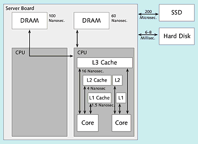
Figure 1.2Access Times
|
Memory |
Access Time in Nanoseconds |
Access Time |
|---|---|---|
|
Hard disk |
6.000.000 – 8.000.000 |
6 – 8 milliseconds |
|
Flash memory |
200.000 |
200 microseconds |
|
Main memory (DRAM) |
60 – 100 |
60 – 100 nanoseconds |
|
L3 cache (CPU) |
~ 16 (about 40 cycles) |
~ 16 nanoseconds |
|
L2 cache (CPU) |
~ 4 (about 10 cycles) |
~ 4 nanoseconds |
|
L1 cache (CPU) |
~ 1.5 (about 3 – 4 cycles) |
~ 1.5 nanoseconds |
|
CPU register |
< 1 (1 cycle) |
< 1 nanosecond |
Table 1.2Typical Access Times
When sizing an SAP HANA system, you should assign enough capacity to place all frequently required data in the main memory so that all critical reading accesses can be executed on this memory. When accessing the data for the first time (e.g., after starting the system), the data is loaded into the main memory. You can also manually or automatically unload the data from the main memory, which might be necessary if, for example, the system tries to use more than the available memory size.
In the past, hard disk accesses usually caused the performance bottleneck; with SAP HANA, however, main memory accesses are now the bottleneck. Even though these accesses are up to 100,000 times faster than hard-disk accesses, they are still 4 to 60 times slower than accesses to CPU caches, which is why the main memory is the new bottleneck for SAP HANA.
The algorithms in SAP HANA are implemented in such a way that they can work directly with the L1 cache in the CPU wherever possible. Data transport from the main memory to the CPU caches must therefore be kept to a minimum, which has major effects on the software innovations described in the next section.
1.2.2Software Innovations
The software innovations in SAP HANA make optimal use of the previously described hardware in two ways: by keeping the data transport between the main memory and CPU caches to a minimum (e.g., by means of compression), and by fully leveraging the CPUs using parallel threads for data processing.
SAP HANA provides software optimizations in the following areas:
-
Data layout in the main memory
-
Compression
-
Partitioning
These three areas are discussed in more detail in the following subsections.
Data Layout in the Main Memory
In every relational database, the entries of a database table must be stored in a certain data layout—independent of whether this representation is done in the main memory (e.g., in SAP HANA) or by following the traditional approach using a physical medium. Two completely different options are available for this: row-based and column-based data storage. SAP HANA supports both approaches. The concepts and their differences are explained next.
We’ll first take a look at row-based data storage in the row store of SAP HANA. In this store, all data pertaining to a row (e.g., the data in Table 1.3) are placed next to each other (see Figure 1.3), which facilitates access to entire rows. Accessing all values of a column is a little more complex, however, because these values can’t be transferred from the main memory to the CPU as efficiently as in column-based data storage. Data compression, which is explained in the next section, is also less efficient with this storage approach.
|
Name |
Location |
Gender |
|---|---|---|
|
… |
… |
… |
|
Brown |
Chicago |
M |
|
Doe |
San Francisco |
F |
|
Smith |
Dallas |
M |
|
… |
… |
… |
Table 1.3Sample Data to Explain the Row and Column Store
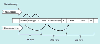
Figure 1.3Illustration of Row-Based Data Storage in the Row Store
Let’s now take a look at column-based data storage in the column store. Column-based data storage is nothing really new; rather, this type of storage was already used in data warehouse applications and analysis scenarios in the past. In transactional scenarios, however, only row-based storage had been used thus far (such as in the row store described already).
Refer to Table 1.3 for a schematic representation of the sample data from Figure 1.4 in column-based storage. The contents of a column are placed next to each other in the main memory. This means that all operations accessing a column will find the required information nearby, which has favorable effects on the data transport between the main memory and the CPU. If a lot of data or all data from a row are needed, however, this approach is disadvantageous because this data isn’t nearby. Column-based data storage also facilitates efficient compression and aggregation of data based on a column.
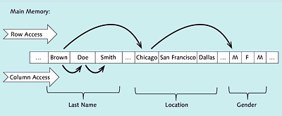
Figure 1.4Illustration of Column-Based Data Storage in the Column Store
As you can see, both approaches have advantages and disadvantages. With SAP HANA, you can specify the storage approach to be used for each table. Business data are almost always placed in column-based storage because the advantages of this approach outweigh its disadvantages. This particularly applies if you need to analyze large amounts of data. However, some tables (or their main access type) require row-based data storage. These are primarily either very small or very volatile tables where the time required for write accesses is more important than the time required for read accesses, or in tables where single-record accesses (e.g., via ABAP command SELECT SINGLE) are the main access pattern.
Compression
The SAP HANA database provides a series of compression techniques that can be used for the data in the column store, both in the main memory and in the persistent storage. High data compression has a positive impact on runtime because it reduces the amount of data that needs to be transferred from the main memory to the CPU. SAP HANA’s compression techniques are very efficient with regard to runtime, and they can provide an average compression factor of 5 to 10 compared to data that hasn’t been compressed.
The compression techniques listed next are based on dictionary encoding, where the column contents are stored as encoded integers in the attribute vector. In this context, encoding means “translating” the contents of a field into an integer value.
To store the contents of a column in the column store, the SAP HANA database creates a minimum of two data structures:
-
Dictionary vector
-
Attribute vector
The dictionary vector stores each value of a column only once. This means that the Gender column for our sample data from Table 1.3 only contains the values “M” and “F” in the corresponding dictionary vector. For the Location column, there are three values: Chicago, San Francisco, and Dallas. The contents of the dictionary vector are stored as sorted data. The position in the dictionary vector maps each value to an integer. In our example, this is 1 for gender “F” and 2 for gender “M”. In the dictionary vector for the location, integer 5 stands for Chicago, integer 6 for Dallas, and integer 7 for San Francisco. Because this value can implicitly be derived from its position (first value, second value, etc.), no additional storage is required.
The dictionary vectors for the sample data from Table 1.4 are displayed in the upper half of Figure 1.5. Only the data shaded in gray are explicitly stored in memory.
The attribute vector now only stores the integer values (the position in the dictionary). Like traditional databases, the order of the records isn’t defined.
|
Record |
Last Name |
Location |
Gender |
|---|---|---|---|
|
… |
… |
… |
… |
|
3 |
Brown |
Chicago |
M |
|
4 |
Brown |
San Francisco |
F |
|
5 |
Doe |
Dallas |
M |
|
6 |
Doe |
San Francisco |
F |
|
7 |
Smith |
Dallas |
M |
|
… |
… |
… |
… |
Table 1.4Sample Data for Dictionary Encoding and Compression
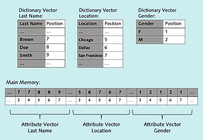
Figure 1.5Dictionary Encoding
The last name “Smith” was placed in the dictionary vector for last names. From its position in this vector, a value can implicitly be derived (the value “9” in our example). This value, again, is now always stored at the position for the last name “Smith” in the attribute vector for the last name; in our example, this is the seventh record of the sample data from Table 1.4. Another example is the location “San Francisco”, which is stored at position 7 in the dictionary vector for the location and appears for rows 4 and 6 in the attribute vector for the location (Table 1.4). The attribute vectors are shown in the lower part of Figure 1.5. In this figure, all three attribute vectors are shown consecutively to show that all data (also the dictionary vectors) are stored in a data stream in the main memory and addressed via memory references and offsets. Here, only the sections shaded in gray in Figure 1.5 are actually stored in the main memory. The row numbers displayed below those sections don’t need any storage space and are again derived implicitly from their position in the attribute vector. They correspond to the position in our example of Table 1.4 (first record, second record, etc.).
The fact that the data are only stored as integer values in the attribute vectors provides the following advantages:
-
Lower storage requirements for values that occur several times
-
Accelerated data transfer from the main memory to CPU caches because less data needs to be transported
-
Faster processing of integer values (instead of strings) in the CPU
Moreover, additional compression techniques can be used for both dictionary vectors and attribute vectors. These are introduced in more detail later on.
For the dictionary vector, delta compression is used for strings. With this compression technique, every character from a string in a block with 16 entries, for example, is stored only once in a delta string. Repeated characters are stored as references.
[Ex]Delta Compression
The following entries are present: Brian, Britain, Brush, Bus. After delta compression, this results in the following: 5Brian34tain23ush12us. The first digit indicates the length of the first entry (Brian = 5). The digit pairs between the other entries contain the information for reconstruction. The first digit indicates the length of the prefix from the first entry; the second digit indicates the number of characters that are appended by the subsequent part. Consequently, “34tain” means that the first three characters from Brian (“Bri”) are used and that four more characters are added (“tain”). “23ush” means that the first two characters from “Brian” are used and three more characters (“ush”) are added. “12us” means that one character from “Brian” is used and that two more characters are added (“us”).
For the attribute vector, you can use one of the following compression techniques:
-
Prefix encoding
Identical values at the beginning of the attribute vector (prefixes) are left out; instead, a value and the number of its occurrences is stored only once. -
Sparse encoding
The individual records from the value with the most occurrences are removed; instead, the positions of these entries are stored in a bit vector. -
Cluster encoding
Cluster encoding uses data blocks of perhaps 1,024 values each. Only blocks with a different value are compressed by storing only the value. Information on the compressed blocks is then stored in a bit vector. -
Indirect encoding
Indirect encoding also uses data blocks of 1,024 values each. For every block, a mini-dictionary is created that is similar to the dictionary vector in the dictionary encoding described previously. In some cases, a mini-dictionary may be shared for adjacent blocks. This compression technique provides another level of abstraction. -
Run-length encoding
With run-length encoding, identical successive values are combined into one single data value. This value is then stored only once together with the number of its occurrences.
SAP HANA analyzes the data in a column and then automatically chooses one of the compression techniques described. Table 1.5 presents a typical application case for each compression technique.
|
Compression Technique |
Application Case |
|---|---|
|
Prefix encoding |
A very frequent value at the beginning of the attribute vector |
|
Sparse encoding |
A very frequent value occurring at several positions |
|
Cluster encoding |
Many blocks with only one value |
|
Indirect encoding |
Many blocks with few different values |
|
Run-length encoding |
A few different values, consecutive identical values |
|
Dictionary encoding |
Many different values |
Table 1.5Overview of Compression Techniques
The memory structures presented so far (consisting of sorted dictionary vectors and attribute vectors with integer values), which might still be compressed in some cases, are optimized for read access. These structures are also referred to as the main store. They aren’t optimally suited for write accesses, however. For this reason, SAP HANA provides an additional area that is optimized for write access: the delta store. This store is explained in detail in Appendix C. In this appendix, another memory structure is also described: indexes. Moreover, Appendix C explains why SAP HANA is called an insert-only database.
Partitioning
Let’s now take a look at the third area of software innovation: partitioning. Partitioning is used whenever very large quantities of data must be maintained and managed.
This technique greatly facilitates data management for database administrators. A typical task is the deletion of data (such as after an archiving operation was completed successfully). There is no need to search large amounts of information for the data to be deleted; instead, database administrators can simply remove an entire partition. Moreover, partitioning can increase application performance by only reading those partitions in which the data required occur (partition pruning).
There are basically two technical variants of partitioning:
-
Vertical partitioning
Tables are divided into smaller sections on a column basis. For example, for a table with seven columns, columns 1 to 5 are stored in one partition, while columns 6 and 7 are stored in a different partition. -
Horizontal partitioning
Tables are divided into smaller sections on a row basis. For example, rows 1 to 1,000,000 are stored in one partition, while rows 1,000,001 to 2,000,000 are placed in another partition.
SAP HANA supports only horizontal partitioning. The data in a table are distributed across different partitions on a row basis, while the records within the partitions are stored on a column basis.
The example in Figure 1.6 shows how horizontal partitioning is used for a table with the two columns—Name and Gender—for column-based data storage.
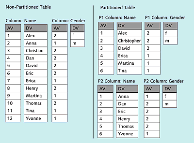
Figure 1.6Partitioned Table
On the left side, the table is shown with a dictionary vector (DV) and an attribute vector (AV) for both the column Name and the column Gender. On the right side, the data was partitioned using the round-robin technique, which is explained in more detail next. The consecutive rows were distributed across two partitions by turns (the first row was stored in the first partition, the second row in the second partition, the third row again in the first partition, etc.).
Partitioning should be used in the following application scenarios:
-
Load distribution
If SAP HANA runs on multiple servers, the data from very large tables can be distributed across several servers by storing the individual partitions of the tables on different servers. Table queries are then distributed across the servers where a partition of the table is stored. This way, the resources of several computers can be used for a query, and several computers can process the query in parallel. -
Parallelization
Parallelization is not only possible across multiple servers but also on a single server. When a query is run, a separate thread is started for each partition, and these processes are processed in parallel in the partitions. Note that parallelization across partitions is only one variant of parallelization in SAP HANA. There are other types of parallelization that can be used independent of partitioned tables. -
Partition pruning
With partition pruning, the database (or the database optimizer) recognizes that certain partitions don’t need to be read. For example, if a table containing sales data is partitioned based on the Sales organization column so that every sales organization is stored in a separate partition, only a certain partition is read when a query is run that needs data just from the sales organization in that partition; the other partitions aren’t read. This process reduces the data transport between the main memory and CPU. -
Explicit partition handling
In some cases, partitions are specifically used by applications. For example, if a table is partitioned based on the Month column, an application can create a new partition for a new month and delete old data from a previous month by deleting the entire partition. Deleting this data is very efficient because administrators don’t need to search for the information to be deleted; they can simply delete the entire partition using a Data Definition Language (DDL) statement.[»]Partitioning to Circumvent the Row Limit
The SAP HANA database has a limit of two billion rows per table. If a table should comprise more rows, it must be partitioned. Each partition must again not contain more than two billion rows. The same limit applies to temporary tables that are, for example, used to store interim results.
Now that you’re familiar with the concept of partitioning and suitable application scenarios, let’s consider the types of partitioning available in SAP HANA:
-
Hash partitioning
Hash partitioning is primarily used for load distribution or in situations where tables with more than two billion records must be maintained. With this type of partitioning, data is distributed evenly across the specified number of partitions based on a calculated key (hash). Hash partitioning supports partition pruning. -
Round-robin
With round-robin partitioning, data are also distributed evenly across a specified number of partitions so that this type is also suitable for load distribution or for very large tables. Round-robin partitioning doesn’t require a key; instead, the data are simply distributed in sequence. If a table is divided into two partitions, for example, the first record is stored in the first partition, the second record is stored in the second partition, the third record is again stored in the first partition, and so on (see Figure 1.6). Round-robin partitioning doesn’t support partition pruning. -
Range partitioning
With range partitioning, the data are distributed based on values in a column. You can, for example, create a partition for every year of a Year column or create a partition for three months of a Month column. In addition, you can create a partition for remainders if records are inserted that don’t belong in any of the ranges of the partitions you created. Range partitioning supports partition pruning.
These partitioning types can be combined in a two-step approach. For instance, you could use hash partitioning in the first step and then, in a second step, use range partitioning within this hash partitioning.