Did you feel unmoored through several chapters without SQL? I get it. Well, we’re back to SQL now. In this chapter, we’re going to go over some advanced BigQuery capabilities that will give you a whole new set of tools to get at your data. After this chapter, I guarantee that the next time you get a juicy business question and a blank console window, you’ll start hammering the keyboard like Scotty in Star Trek IV keying in the formula for transparent aluminum.1
Fair warning: There’s some JavaScript in this chapter. I’ll give you a heads-up so you don’t crash into it while enjoying your SQL reverie.
Analytic Functions
As you become familiar with subqueries, joins, and grouping, you will start to think with more and more complexity about how to get at the data you need for analysis. Layering in capabilities outside of BigQuery, like Cloud Functions and Dataflow SQL, you can conceive of multiple solutions to any analysis problem.
But there’s one tried-and-true toolbox for doing data analysis that we haven’t explored yet. Analytic functions have been critical to OLAP workflows for decades, and they’re not going anywhere anytime soon. To really bring your game up to par, learn and use analytic functions.
Analytic functions are also sometimes called window functions or even OLAP functions, so if you’ve heard of them in that context, I’m referring to the same thing here. Many data engineers avoid them because of the unfamiliar syntax. When I was a junior database developer (at some point in the undisclosed past), I got nervous whenever I opened up a stored procedure and saw OVER, ROW_NUMBER, or the other keywords that signal a query using analytic functions. Databases were the most expensive resource, and so writing queries that performed poorly or used too much memory could affect production system operations. It often seemed safer to rewrite them using multi-statement subqueries and joins, especially when they were running in production.
So those things are, on balance, still true. Analytic functions still run more slowly on the whole; they can always be refactored using subqueries and joins; and many data engineers avoid them. I don’t blame you for loading your table into Python with the BigQuery API and scripting out your analytics. In reality, you do what is most efficient for you with the tools you have. People got by before BigQuery too. (And when I was a junior database developer, a cloud was still a fluffy thing in the sky that sometimes rained on you.)
Definition
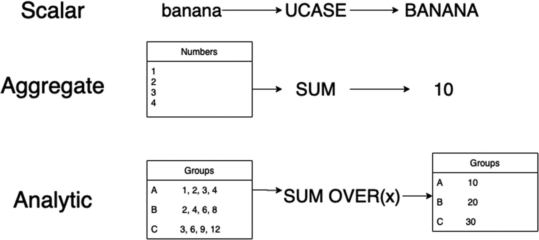
Scalar, aggregate, analytic
As you can see, the analytic function retains the grouping inside the partitions. The analytic function runs an aggregate across multiple rows, but each row gets a result.
Window Frames
Imagine a sheet of paper with a printed table on it. Choose a single row in the middle of the table, which will be the row being “evaluated.” Then, use two more sheets of paper—one to cover some of the rows above the evaluated row and one to cover some of the rows below. The rows that you left uncovered are your “window frame.”
This is essentially what a window frame does when processing an analytic function. As each row is evaluated to assign the result, the query uses the window frame to decide which rows should be included in the input grouping. The pieces of paper move along with the row under evaluation to expose different rows as the analytic function proceeds.
The OVER clause defines the window frame. It’s also acceptable to use the entire input set as a single frame.
Partitions
In addition to the window frame, you can also use PARTITION BY to group rows by key. The last step that GROUP BY takes to collapse those rows does not occur; they are held in separate partitions. You can also use ORDER BY when defining the partitions; unlike a query-level ORDER BY, this version specifies the order within each partition.
Because we’ve been talking about partitioned tables in BigQuery so much, I want to point out that this is not a related concept. This type of partitioning refers to the bucketing of sets of input rows from a single query result.
Order of Operations
All GROUP BY and regular aggregate functions are evaluated first.
Partitions are created following the expression in PARTITION BY.
Each partition is ordered using the expression in ORDER BY.
The window frame is applied.
Each row is framed and the query is executed.
The partition is a stricter boundary than a window frame; the frame won’t span multiple partitions. Once the partitioning step has occurred, you can imagine that these are actually all separate tables grouped by the partition—they will not interact.
Many analytic functions do not support windows; in this case, the window frame used is the entire partition or input set.
Numeric Functions
One rule of thumb for identifying a business problem that might benefit from an analytic function is when you hear someone ask for “the most/least X for each Y.” The “X” is your ORDER BY expression, and the “Y” is your PARTITION BY.
For numeric functions, you’ll always be doing some sort of precedence ordering. Window frames aren’t allowed for numeric functions, so the analytic function will always be operating across the entire partition.
ROW_NUMBER
Before we go too crazy, let’s look at the simplest of the analytic functions, ROW_NUMBER. All ROW_NUMBER does is return the ordinal of the row within its partition. While this is pretty simple, it’s very powerful and gives us an easy way to order subsets of a query. It’s otherwise surprisingly nontrivial to assign row numbers to returned rows.3
Partition the Products table by ShoeType, creating one partition per type.
Order each partition by the price of the shoe, highest to lowest.
Return one row for each shoe type and color and a number indicating where it fell in the price order.
For ROW_NUMBER, you actually don’t need to specify an ORDER BY at all; without one, the results are non-deterministic. You would still get the benefit of the partitioning and a unique ordinal for each type of shoe.
RANK
RANK is substantially similar to ROW_NUMBER , except as the name implies, it gives a ranking. That means it’ll behave like a ranking in a sports division; if the ORDER BY has two rows that evaluate the expression identically, they’ll get the same rank.
To apply to the preceding example, if two shoes had the same price, they’d get the same rank. ROW_NUMBER() always assigns a distinct value to each row in a partition.
DENSE_RANK
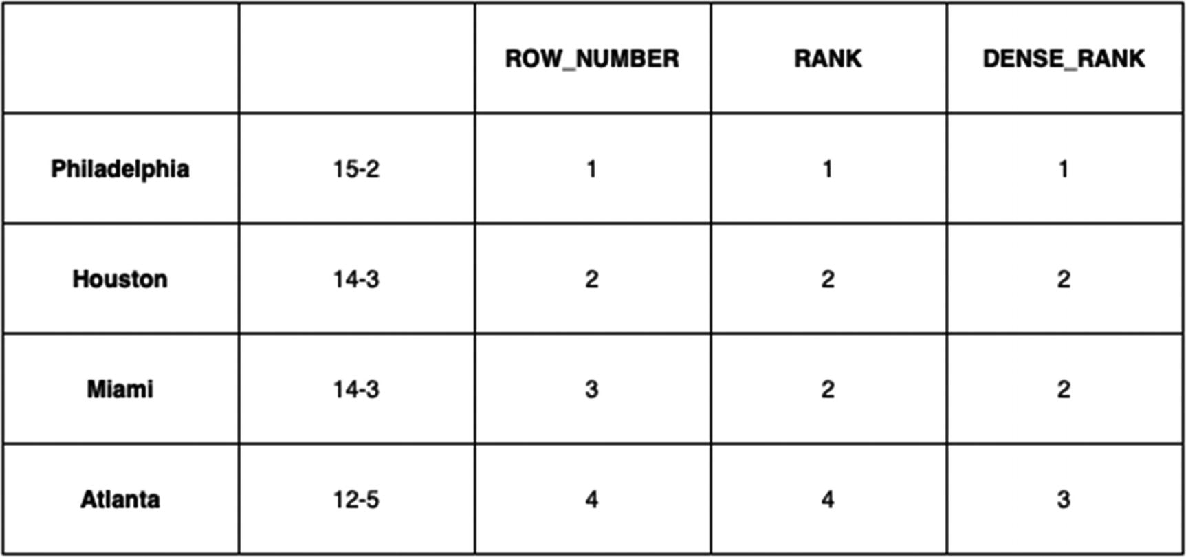
Showing a baseball division
Basically, RANK is what you’re used to seeing in sports standings (“Houston and Miami are tied for second with Atlanta in fourth”), and DENSE_RANK is what you’d see in a statistics report (“Houston and Miami have the second highest count of rabid zombies, with Atlanta in third.”)
PERCENT_RANK/CUME_DIST
These two functions are closely related in that they both return a fraction between zero and one indicating the row’s position in the partition.
PERCENT_RANK returns the percentage of values that are less/more (come earlier in the partition) than the current row. So the first row in a partition will always be 0; the last row will be 1. The formula is (RANK() – 1)/(Partition Row Count – 1).
CUME_DIST returns the percentage of the row within the partition, or just a straight fraction of RANK() over the partition row count. The first row in a partition will always be 1/n, where n is the number of rows in the partition; the last row will always be 1.
Window Frame Syntax
See, that wasn’t so bad. I always find that a new syntax looks daunting until I actually sit down with it and learn it, and then the next time I see it, I’m pleasantly surprised to discover that now it means something to me. SQL is kind of like that.
Before we get into navigation functions, we should cover how you specify a window frame. Reading this syntax can get a little hairy. To simplify as much as possible, don’t think about partitions for the moment; just think about a single table of, say, 48 rows, being iterated sequentially. For each row, we use the window frame to determine which rows around it we use to evaluate the analytic function. Using the syntax, we can specify pretty much any set we want. Lastly, remember that the frame moves relative to the row under evaluation. Each of these frames then constitutes a tiny table we’ll do a regular aggregation on. Since the frame moves, the same rows will be included in multiple frames—just think about it as an iterative process over each row, and it won’t be confusing.

48-row table with hourly measurements
I’ve specified a window that will be three rows wide—the row under evaluation, the row before it, and the row after it. (At the top and bottom of the table, my window will only be two rows wide, since there are no rows above the top or below the bottom.)
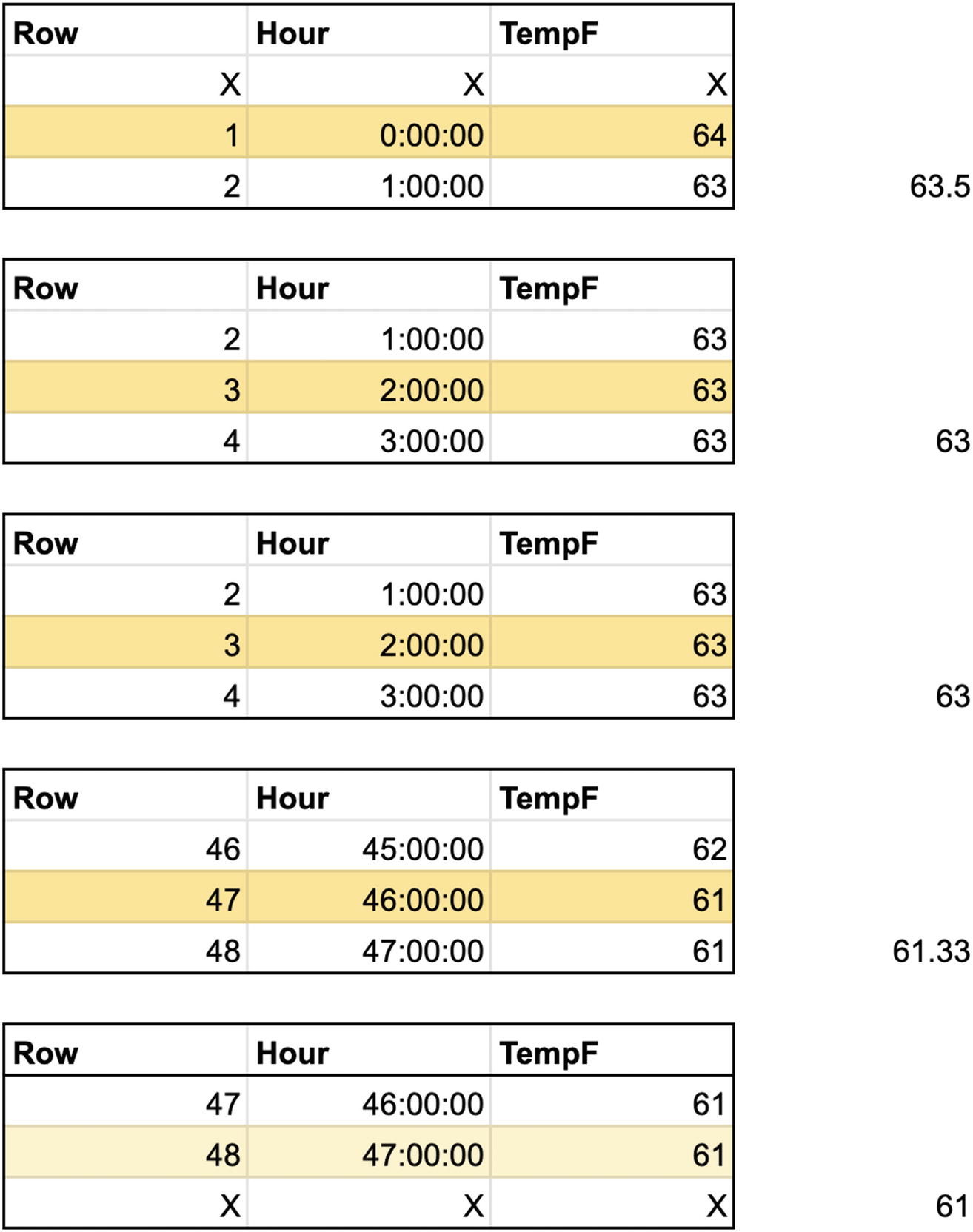
Shows the frame for each row under evaluation
Then for each frame, we perform the average of current temperatures in the specified rows and apply the result to the row.
(This is more useful when I’ve partitioned the table and want to calculate a value for each partition; you’d also generally use it in combination with other analytic functions. Otherwise, you could just select the whole table and then get the aggregate in a GROUP BY.)
This specifies a logical window frame that goes 30 days into the past and 30 days into the future. It doesn’t matter how many rows that comprises; it will use the value of Date to decide.
Back to that implication, if you knew for certain that you only had one row for each day and no days were skipped, then this RANGE would be equivalent to a ROW BETWEEN 30 PRECEDING AND 30 FOLLOWING. It’s easy to think you need to prepare your input to fill in the gaps so that you can do a ROW window, but this is not necessary. You can work directly with any expression in the partition by using the RANGE option.
Navigation Functions
I find this label a little questionable, but the idea is that the value they yield is produced using data from another row than the row being evaluated. In that sense, the function must “navigate” to a different row to get the result. The navigation is bounded first by the partition and then by the frame. Then the analytic function is applied over the frame and the result applied to the row under evaluation.
Using this navigation idea, we can actually consider most of the functions together by describing where they navigate to in order to calculate the value. Then we can dive into each and see how they might be useful.
FIRST_VALUE returns the value for the first row in the frame.
NTH_VALUE returns the value for the row at the position you specify in the frame.
LAST_VALUE returns the value for the last row in the frame.
LAG returns the value for a row earlier in the frame by offset.
LEAD returns the value for a row later in the frame by offset.
Table is partitioned by your PARTITION BY.
Each partition is ordered by your ORDER BY.
- Then, for each partition
Each row is evaluated in order.
For each row, the frame is set based on your framing options.
Based on the frame, the navigation function chooses the row to look at, relative to the current row.
All rows in each partition are rejoined together, producing your output range.
Which day had the highest temperature each month?
Which day had the lowest temperature each month?
Which employee has the next-most tenure for each employee by department? (Rephrased naturally, which employees started around the same time?)
Which movie comes two movies later in each series, by franchise?
What book came out closest to the beginning of the same year as each book, by subject?
See if you can construct the PARTITION BY, ORDER BY, and window frame, either ROW or RANGE, for each of these questions. While all of these examples have a PARTITION BY, you can also use the full table and often calculate useful information and the table level. The partitioning just gives you an extra level of grouping to work with, so you can answer the same question for every piece of data in the input.
No self-join, no messy aliases, and a lot easier to modify if it turns out you need something besides the name. Also, this query only works for an input of a single series. As soon as you add “for each series” to the question, the analytic version just needs “PARTITION BY Series.” Doing this with regular SQL is substantially more complicated, involving the construction of a subquery and/or self-join.
Having fun yet?
Aggregate Analytic Functions
The last class of analytic functions are those that do double duty as regular aggregate functions. So good news: You already know these. To use them as analytic functions, you just specify them with an OVER clause instead of paired to a GROUP BY clause.
Using the WITH clause, generate all the numbers from 1 to 100 and put them into a table named numbers. Each number is referenceable by the column num.
- Using this table, select three things:
The original number
A moving average using the current number and the two numbers preceding it
The cumulative sum of all numbers up to the current number (i.e., a running grand total or, if you like math, term n+1 of the triangle number function)
Copy this query into BigQuery and run it. It’s self-sufficient since it generates its own data for the functions, so you don’t need to do any preparation.
Change the numbers the GENERATE_ARRAY sequence produces. Try negative numbers or larger or smaller ranges. Add a third parameter to the function, which specifies the step between elements. For example, GENERATE_ARRAY(1, 100, 2) will produce the sequence [1,3,5,7,...]. Watch what the RunningTotal begins generating when you do this! It’s an obvious but perhaps nonintuitive result.
Try floating-point numbers in GENERATE_ARRAY. You can step over decimal numbers by decimal steps.
Change the window frames of the average and sum functions to calculate moving averages or sums. Try extending the frame to the entire table.
Try RANGE windows instead of ROW windows. Notice what happens to the results if you only replace “ROW” with “ORDER BY num RANGE” vs. what happens if you change the GENERATE_ARRAY sequence as well as the frame type.
Add some other analytic functions to make more columns and explore their results as well. Use the instructions in Chapter 9 to guess what they’ll do in this context. Some interesting ones to try here are COUNT, COUNTIF, and ANY_VALUE. (ANY_VALUE is especially interesting because you can peer into the soul of BigQuery’s determinism. The value doesn’t change over repeated runs, even though it could, according to the rules.)
Change the expression in the analytic function without changing anything else. For example, what happens when you do SUM(num*num) OVER (ROWS BETWEEN UNBOUNDED PRECEDING AND CURRENT ROW)?4
Try adding partitions to one or all of the columns. Experiment with different values for partitioning.
Generate multiple sequences into the numbers table, for example, all odd numbers from 1 to 100 and all even numbers from 1 to 100. Try ordering by one column and using analytic functions over multiple columns.
Start adding back in the navigation and numbering functions we already covered. What can you do with ROW_NUMBER() as a column? With LAG and LEAD?
I heard you hammering on the keyboard just now. You didn’t even notice, but my guarantee came true! The questions you can answer with a single query employing analytic functions are amazing. Sorry, Google. The BigQuery documentation just doesn’t do it justice in this case.
Analytic functions really add a whole new class of power to what you can do with SQL. With some syntax variations, all modern OLAP systems support this, so you’ll also be able to take this knowledge and use it in other data warehouses. As I suggested earlier, getting this deep with SQL can truly change the way you see the world!
BigQuery Scripting
When all else fails, BigQuery still has your back. BigQuery supports the full set of scripting commands too. So when your coffee mug is empty and you just can’t translate a recurrence relation into an analytic function, procedural programming will still be there for you.
In BigQuery’s case, scripting brought about multi-statement requests too, which had been lacking and made it somewhat difficult to do complicated transformations in a single call. This also gives you the normal trappings of variables, assignments, loops, and exceptions.
If you’ve worked with PL/SQL, T-SQL, or other procedural implementations of SQL, these concepts will all be familiar to you. And if you’ve worked in other languages and are new to SQL, they will still be relatively familiar to you.
Blocks
BigQuery uses BEGIN and END as the keywords for a block. A block signifies scope for variables declared and exceptions thrown inside of it. All statements inside a block must end with semicolons.
Variables
Variables are declared using DECLARE, and all variables must be declared before use. You can declare a variable in any type supported by BigQuery, and you may declare multiple variables of the same type with the same statement. Variables can be assigned a default value, which they will retain until you SET some other value. If you don’t specify a default, the variable will be initialized to NULL.
You can also set the DEFAULT to be the result of a subquery, which is a convenient way to avoid a SET statement directly after the declaration.
There are no higher-level language features like constants, pointers, object orientation, classes, private variables, and so on.
Comments
IF/THEN/ELSEIF/ELSE/END IF
You can set the value of multiple variables inside the same statement by parenthesizing both sides of the assignment.
You can combine conditions in the IF statements with boolean logic.
You can use FORMAT to insert variables into a string.
RAND() is the pseudo-random number function in BigQuery; it generates a FLOAT between 0.0 and 1.0.
Control Flow
BigQuery has three primary control flow constructs, LOOP, WHILE, and exception handling. If you want to implement anything more complicated, like a FOR loop, you’ll have to do it yourself.
LOOP/END LOOP
Loops run forever unless you BREAK (or LEAVE) them. This isn’t the first opportunity you’ve had to make an infinite loop in BigQuery, but it’s the easiest one that’s come along so far. The maximum query duration is 6 hours. I’ll just leave those two facts there and keep going.
takes 0.3 second and runs a single statement. Just because you have loops available to you doesn’t mean you should immediately rely on them when there is probably a SQL solution that uses sets. Note: LEAVE and BREAK are completely synonymous keywords.
WHILE/DO/END WHILE
This query takes roughly as long as the LOOP version and is roughly as useful.
Exception Handling
If you run this sample, you’ll actually see the results of both queries in the display: the failed query trying to divide by zero and the “successful” query returning the error message.
@@error.message gives you the error message.
@@error.statement_text gives you the SQL statement that caused the exception—very helpful for debugging, especially when it’s an obvious division by zero.
@@error.stack_trace returns an array of stack frames and is intended for programmatic traversal of the error’s stack trace.
@@error.formatted_stack_trace is the human-readable version of the stack trace, and you should not do any processing on the string. Use .stack_trace instead.
Using RAISE inside a BEGIN will cause flow to be transferred to the EXCEPTION clause, as usual. Using RAISE inside of an EXCEPTION clause will re-raise the exception to the next error handler, eventually terminating with an unhandled exception if nothing intercepts it.
RETURN
Return ends the script from wherever you invoke it. It works anywhere inside or outside of a block, so if you use RETURN and then continue the statement list, those subsequent statements will be unreachable.
Stored Procedures, UDFs, and Views
Scripts can be pretty useful on their own, even when run interactively. However, the name of the game here has always been reusability. At the GCP level, we’re looking to manage our imports and streams so that they can be used across a variety of incoming data. When we write table schemas, we want them to describe our data in a durable way so that they can hold all the types of relevant entities and grow with our business.
The way we do that with scripts is to encapsulate them in stored procedures and user-defined functions, or UDFs. (Views are a little different, but they’re traditionally all taken together so we’ll honor that approach here.)
Stored Procedures
A lot of ink has been spilled discussing the pros and cons of stored procedures, whether we should use them at all, and why they’re amazing or terrible. Despite the on-and-off holy war about the value of stored procedures over the last couple decades, they’ve never gone away. It is true that they still leave something to be desired when it comes to versioning, source control, and deployment practices. But the tools to manage all of those things have been around for nearly as long as stored procedures themselves. The failure to embrace these processes is in large part a function of how data organizations operate.
The purpose of showing all of the things you can do with integration to BigQuery, other services, and other paradigms was, in large part, to show that you have the best of both worlds. You can maintain your Dataflows, cloud functions, and transformation scripts in the most cutting-edge of continuous integration systems. You can ensure that all of your critical warehouse activities are documented, repeatable, and resistant to error.
There is still room for stored procedures and UDFs in that world too. While I’d be significantly less likely to recommend or build a massive inventory of chained procedures to perform production line-of-business tasks, I’d also store any reasonable, reusable script in a procedure for use by other analysts and applications. Stored procedures are great for containing complex analytic function work. While a lot of business logic has migrated out to API or serverless layers, this core online analytics work belongs with SQL.
Ultimately, I think if stored procedures weren’t a sound idea architecturally, Google wouldn’t have taken the trouble to add support for them into BigQuery. This isn’t holdover functionality; they were only introduced in late 2019.
Key Principles
IN: Like an argument passed to a function
OUT: Like a return value
INOUT: Like a pass-by-reference
There’s no encapsulation of methods, so if you SELECT inside a stored procedure, it will be emitted as if you were running an interactive command. You can use this if you just want the client calling the stored procedure to get results back without the use of parameters.
Temporary Tables
We haven’t needed temporary tables for much so far; BigQuery basically creates a temporary table to hold results every time you run a query. But within stored procedures, you often want a place to store the intermediate results while you work. You can do this simply with “CREATE TEMP TABLE AS,” followed by the SELECT query with which you want to initialize it. When you’ve finished with the table, be sure to “DROP TABLE TableName” so that it doesn’t persist anywhere.
Syntax
Note that I used “CREATE OR REPLACE,” instead of just “CREATE,” so that the procedure will alter itself as you make changes to it. This procedure just selects a random number between 1 and the Maximum parameter. After creating it, the last three lines show a sample invocation, where a variable is created to hold the result, the procedure is called, and the answer is returned.
Also note the use of a subquery to set the value for the answer. Since “Answer” is declared as an OUT parameter, I can assign to it directly. One important note: BigQuery actually doesn’t do any checking to prevent you from assigning to an IN variable. If you forget to declare an argument as “OUT” and then SET it anyway, the variable will be updated within the scope of the stored procedure, but it will not be emitted to the caller. This doesn’t cause an error at parse or runtime, so watch out for it.
User-Defined Functions
User-defined functions are also stored code that you can use inside other queries, but they don’t stand alone like stored procedures do. They are functions you create that behave the same as any of the functions in the standard library, like UCASE() or LCASE() or the RAND() we just used earlier. (Oh, and as promised, here’s your warning that the JavaScript’s coming up.)
This will return 15, which is magically the correct answer to 10 + 5. While the example is simple, it’s all that’s really needed to convey what a user-defined function would typically do. You are likely to have operations in your business that have fairly simple mathematical definitions, but which are critical in your business domain. Rather than hardcoding them all over all your queries, this is an easy way to make those operations consistent.
For example, if your business consists of a lot of travel between the United States and Canada, you may want a simple unit conversion operation to go between miles and kilometers, if only to make the code more readable and avoid the specification of the constant each time.
On the other end of the spectrum, you can make arbitrarily complex functions for statistical and mathematical operations. Whatever operation you need that BigQuery doesn’t provide built in, you can create it.
ANY TYPE
we can now invoke the function across any data type we like. BigQuery can automatically figure out based on our operations which types are valid. So with this modification, I can run AddFive(10.5) and get back 15.5 with no problem. But if I try to AddFive(“help”), BigQuery catches it and tells me I need a signature of NUMERIC, INT64, or FLOAT. (Were you expecting the result “help5”? What is this, JavaScript?)
User-Defined Aggregate Functions
What if you want to define your own aggregate functions? There’s no native support for this, but there is a way to fake it.
This creates a function that takes an array of numerics and calculates the average. You could of course write SUM(x)/COUNT(x) or any other type of aggregation you would want to perform.
The template analysis will restrict the input to an array of numerics, because the AVG aggregate needs numeric input, and the UNNEST function needs an array. But you still can’t use this fake_avg function directly, since you still need to generate the array of numerics.
Unfortunately, that syntax is starting to look a bit less natural.
JavaScript User-Defined Functions
User-defined functions have another trick up their sleeves, and that’s the ability to call out to any arbitrary JavaScript. This feature is fantastically powerful, because it’s basically like being able to write any procedural code you might need, all within the scope of values across rows. This opens up all kinds of avenues. Even more interestingly, it gives you the ability for the first time to share code with applications running in the browser or on NodeJS (with limitations, of course). We’ll discuss that possibility after we go over the basics.
This does the same thing as our SQL UDF, but now we’re doing it in JavaScript. Some other things have changed here too. First of all, we’re using FLOAT64 as the type now; that’s because JavaScript has no integer-only data type. FLOAT64 goes over as NUMBER, and that’s one important gotcha—type mapping between SQL and JavaScript.
The second thing you’ll notice is that the RETURNS clause is now required. BigQuery can’t infer what kind of type you’ll be returning unless you give it the conversion back into SQL. Interestingly, you can return INT64, but if your JavaScript tries to return a number with a decimal part, it will get unceremoniously truncated on its way back.
Lastly, you’ll notice the odd-looking triple-quote syntax. If you’re writing a single line of JavaScript, you can use a single quote, and indeed we might have done that in our example. But it’s probably best to be explicit and use the triple-quote syntax, both because it prevents an error later where we try to add another line to the function and because it signals to any other readers that something unusual is going on here.
Limitations
There is no browser object available, so if you’re taking code that you ran in a web browser, you don’t get a DOM or any of the default window objects.
BigQuery can’t predict what your JavaScript is going to do nor what would cause an output to change. So using a JS UDF automatically prevents cached results.
You can’t call APIs or make external network connections from a UDF, as fun as that sounds.
There’s no way to reference a BigQuery table from inside of the JavaScript—you can pass structs in, and they will appear as objects on the JS side, but you can’t arbitrarily select data.
You also can’t call out to native code, so don’t go trying to use grpc or anything. But you can use WebAssembly to compile native C or Rust into JS and then use it in SQL. (But do you really want to?5)
External Libraries
This example will fetch the library from the Google Storage location you specify and include it in the processing for your function. Then you can execute any function the library defines as if you had written it inline.
If you’re familiar with the Node ecosystem, your next question is likely, “But can I use npm packages?” The answer is sort of. You’re still subject to all of the memory, timeout, and concurrency limitations, but all you need to do is get the package to Google Cloud Storage. The best way to do this is Webpack, which works totally fine with JS UDFs.
Other BigQuery users, already recognizing the conceptual leap this represents, have begun repackaging useful BigQuery functions as Webpack JavaScript and publishing those as repositories. It seems fairly likely that people will begin creating public Cloud Storage buckets with these libraries available for referencing, much as popular JavaScript plugins began appearing on CDNs for browsers, but I haven’t seen anyone doing this yet. Maybe you could be the first.
Views
A view is best summarized as a virtual table. Typically, views don’t actually move any data around; they are, as implied, a “view” into the columns of one or more tables. In the case of BigQuery, views do store the schemas of the underlying tables they use, so if you modify the table schemas, you should also refresh the view.
Creating a view is easy; whenever you run any query in the interactive window, directly next to the “Save Query” button is another button labeled “Save View.” Clicking that will ask you to specify the dataset to store the view in and the name of the view.
To edit a view, you can double-click it and go to the Details tab. At the bottom of that tab, you will see the query used to generate the view and can edit and resave it.
Materialized Views
Materialized views, on the other hand, are views that actually collate and store the results of a query. You can use materialized views to replace any “reporting” tables you create with an automatically refreshing, precomputed version.
Materialized views have substantial advantages for data that is frequently accessed. They even pair with streaming (see Chapter 6) to run aggregation on top of incoming data for real-time analysis.
Unlike regular views, materialized views can only use a single underlying base table. Their primary use is to perform various grouping and aggregation on that table to have it available at all times. (Unfortunately, you can’t use analytic functions in a materialized view yet.)
After you create a materialized view, BigQuery will automatically begin refreshing the data from the underlying table with the query you wrote. From now on, whenever you change the data in the underlying table, BigQuery will automatically invalidate the correct portions of the materialized view and reload the data. Since this use case is so tightly tied with streaming, BigQuery also understands how to invalidate and read from partitions.
Advantages of Materialized Views
Materialized views give you a substantial speed boost on your query aggregation. Not only do they improve the performance when querying the view but BigQuery will automatically notice speed improvements in queries to the base table and reroute the query plan to look at the materialized views.
Also, unlike waiting for a scheduled query or an analysis trigger, the data in a materialized view will never be stale. This creates a natural pairing with high-velocity streaming. Several examples in Chapter 6 would be improved by placing a materialized view on top of the ingestion table in order to get automatic aggregation.
Disadvantages of Materialized Views
One potential disadvantage is cost. Since you pay for the query which refreshes the view on underlying table updates, you can transparently incur extra costs just by performing regular operations on the base table. You can also have multiple materialized views pointing at the same table, so basic operations will incur a multiple of cost. Similarly, since the data for the materialized view constitutes a separate copy, you pay for its storage as well.
Another disadvantage is keeping track of your materialized views. BigQuery won’t notify you of a constraint failure if you delete the base table.
Finally, you can’t perform some normal table operations on a materialized view. For example, you can’t join other tables or use the UNNEST function.
Automatic vs. Manual Refresh
You can still use materialized views in concert with your existing maintenance processes. This also mitigates the potential cost risk, since you’ll be controlling when the view updates. (Of course, then you also take back responsibility for keeping the data fresh, so you can’t have everything.) You do this with “OPTIONS (enable_refresh = false)” when you create the table.
Summary
Analytic functions, or windowing functions, give you the ability to express in a few lines of SQL what would take complicated subqueries or self-joins to replicate. Using various types of analytic functions, you can evaluate conditions over partitions and window frames to generate groupings of data without collapsing them as a GROUP BY clause would do. Through numerical, navigation, and aggregate analytical functions, we looked at a variety of ways to order and analyze your data. Beyond that, we entered the realm of scripting, with which you can write constructs using procedural language that are not easily expressible with SQL. Using SQL scripting, you can create powerful stored procedures and user-defined functions, even replicating the usefulness of aggregates. We also looked at the ability to write user-defined functions in JavaScript and referencing external libraries available in the vast ecosystem of npm packages. Lastly, we looked at both traditional and materialized views and how they can lower maintenance operations for the streaming of aggregate data.
You now have a wide breadth of information on the power of SQL for data warehouses, as well as the integration of special BigQuery capabilities and other Google Cloud Platform features. Despite that, we still have a few areas of BigQuery we haven’t even touched yet.
In the meantime, the next several chapters are back to the operational and organizational aspects of supporting your data warehouse. Having secured the ongoing success of your data project with ever-increasing insight, it’s time to look at the long term. In the next chapter, we’ll be looking at how you can adapt your warehouse to the ever-changing needs of your business—and hopefully its continued growth and success as well.