You’ve built the whole warehouse, loaded and streamed the data, set up your workflows, and defined your warehouse’s roadmap for the next several months. You probably feel pretty accomplished, and you know now what you have to do to make your data program a success. You also have a massive amount of data pouring into your system—and I’m sure you’re anxious to do something with it.
In this part, we’ll touch on several other Google services that will be useful to you in dealing with your data, making it accessible to your users, and defining automated tasks to limit the amount of manual work you have to do. We’ll discuss scheduling, functions as a service, logging, and monitoring. Combining these additional tools with the ones you have already will free you to focus on the actual work of analyzing your data. After that, we’ll go into the analytic functions.
But before we get there, let’s turn our attention to all of the power you now have available in BigQuery itself. Remember the goal of your data program is ultimately to take all of this raw data, turn it into information, and productively use that information to generate insights. The hard part was getting all the data into one place to begin making “information” out of it.
In order to work effectively with BigQuery, you will need a working understanding of SQL. This means working with SQL both in the ANSI-compliant sense and the BigQuery-specific concepts that make it so powerful. In this chapter, we’ll run the gamut from basic SQL concepts through querying nested columns, partitions, and many different underlying data types. Buckle up. There’s a lot to talk about!
A navigation note: If you’re already familiar with SQL, you can skim this chapter. For BigQuery specifically, nested data and partitions may be of interest. I’ve reserved advanced discussion around analytic functions for later in this text, so you can skip this chapter entirely if you are looking for that.
BigQuery SQL
Yep, still works. The big difference between Chapter 1 and now is that now you also have your own datasets to run queries against, and they’re likely to be more useful to your particular business domain than tree species (unless you work for the New York City Parks and Recreation Department, in which case maybe these are also your datasets).
This query demonstrates most of the basic principles of how SQL works, but it’s really only scratching the surface of the kinds of queries you’re likely to write. And it doesn’t even begin to touch all of the other database objects you can use to compose your queries into complicated functional units. And even then, it doesn’t cover some of the tips and tricks you might use to operate on extremely large datasets. BigQuery is designed to operate up into the petabyte range. As your data gets larger and larger, you will have to start to understand what’s happening behind the scenes in order to optimize and understand your query performance.
Querying Basics
As we covered in Chapter 1, a query that retrieves information from a database always has the same anatomy. You SELECT data FROM a table WHERE certain conditions are true. Everything else modifies that basic concept.
Let’s revisit the other concepts from the sample query, with more information about their options. For grouping, which is far more complex and has other associated keywords, we’ll cover the basics here and then go deeper in the “Aggregation” section later.
Limits
Using LIMIT and OFFSET to restrict the number of rows returned or to page through the data is a critical BigQuery concept. When your tables have billions of rows, failing to specify a limit for the data returned could result in gigabytes of results. This isn’t cheap or fast. In general, always use a limit on your data unless you are returning a static value set that you know to be small.
Limits and offsets both have to be positive numbers. And unless you specify an order, the rows that will be returned are non-deterministic; it’s simply the first qualifying n rows the query processor encounters.
Ordering
Applying an ORDER BY specifies the sort order in which you want to see the results. In combination with a LIMIT, the ordering is applied first, and then the results are restricted to the top n rows.
You can sort either ascending (the default) or descending, and you can sort by multiple columns using both ascending and descending.
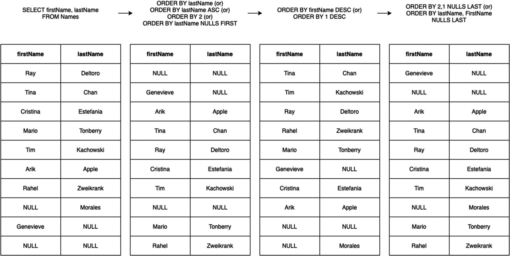
ORDER BY examples
Note that in the last example, instead of using column names, we used numbers. This lets you sort by columns where 1 represents the first result column, 2 the second, and so on. Prefer named sorts over numbered columns, solely because if you change the number or order of the columns in the SELECT statement, the sort behavior will change too, usually unintentionally. (But for scratch queries, it does save you the trouble of retyping the column names, especially when they have been aliased or joined or you’re doing a star SELECT and you don’t remember the name of the column.)
BigQuery also supports choosing whether you want NULL values to appear before or after the non-NULL values. You can configure this with the parameter “NULLS FIRST” or “NULLS LAST.” The default behavior is nulls come first for ASC ordering and nulls come last for DESC ordering.
Note that in BigQuery, certain data types are “unorderable.” These types are STRUCT, ARRAY, and GEOGRAPHY. You’ll get an error if you attempt to include columns of these types in your ORDER BY clause. This is because for the first two types, there’s no top-level value to sort by; they are multivalued. For GEOGRAPHY, it is because there is no canonical ordering for spatial data types. The operation for ordering New York, Chicago, and Los Angeles by location is undefined. (You can, of course, order by distance from or to a given point, and we’ll be looking at that later.)
Grouping
You will also want to group matching data together in order to perform aggregate functions on it. In the sample query, we used grouping to ensure that we only got one result per name. In the raw table, each name appears for each year. In order to find the most popular names, we needed to know, when you looked at each name, which one had the highest number across the datasets.
to immediately show you the slowest pages on your site. Aggregate analysis is the bread and butter of reducing giant datasets into usable information.
MAX: Return the maximum value in the group.
MIN: Return the minimum value in the group.
SUM: Return the sum of all values in the group.
AVG: Return the average of all values in the group.
COUNT: Return the number of values in the group.
With a little bit of creativity, you can actually write your own aggregate functions by piggybacking on the ARRAY_AGG aggregate function. BigQuery doesn’t have official support for this, but we’ll talk about this sort of thing in Chapter 13.
Additional Options
There are additional clauses you can supply to SELECT that we haven’t yet covered.
Star Queries
This has come up a few times, but I’ll iterate it for completeness. Using the * character in a SELECT indicates that you want all of the columns from a result set.
If you use it in a single table query, that is, SELECT * FROM Table, you’ll get all of the columns in Table. Using it in a query that has joins or subqueries will get you all columns in the combined set, that is, SELECT * FROM Table JOIN Table2… JOIN Table3… JOIN TableN will get you all columns from all the tables.
will get you all the columns in table A, but just the Name column from table B.
As we’ve covered before, selecting all the columns is generally not best practice for production queries. Column restrictions are the primary way to avoid accessing (and paying for) unnecessary data. Additionally, it’s quite brittle, since any change in column ordering or column renaming will break the query. It’s good for exploratory data analysis when you don’t remember the names of all of the columns and you want to get a sense of the data.
To get a sense of this in BigQuery, try writing the same query against a large table using a few column names and then by using *. You will see the data estimate skyrocket. For example, running the preceding trees query estimates 12.5 MB of processing; the same query with * is 223.1 MB.1
EXCEPT
The EXCEPT modifier allows you to use the SELECT *, but exclude specific columns from the result set. At least in BigQuery, this is useful for seeing query results in a more compact way by excluding nested columns that can make it hard to read.
REPLACE
The REPLACE keyword allows you to do a sort of batch aliasing of column names. This is an interesting concept for * queries because you can rename certain columns without remembering to name them in the SELECT statement itself.
Especially in a highly denormalized table as BigQuery is likely to have, it’s a nice feature to be able to rename a few out of a hundred of column names without having to specify all hundred names first.
DISTINCT
The default behavior of a SELECT query is SELECT ALL, which means return every row in the set, including duplicates. The purpose of DISTINCT is to filter duplicate rows from the result set and give only one copy of each.
Specific to BigQuery: DISTINCT cannot do comparisons on STRUCTs or ARRAYs, and thus you cannot run one of these queries if you are returning one of those data types.
WITH
WITH is a prefix you can place before SELECT to create a temporary named query result you can use in the following statements. It can be easier to read than a subquery, especially when you need an intermediate result with aggregation to perform additional processing on.
In standard SQL, you can also use WITH to join the table to itself, creating a recursion. BigQuery does not support this, and I honestly shudder to think about recursively self-joining a petabyte-size table.
WITH must be immediately followed by its SELECT statement; it cannot stand alone. The following query counts the number of “Kinds” in a table and uses it to select the row with the highest count. This could also be written as a subquery:
Querying the Past
There’s also one additional feature that FROM has, which is that you can use it to look at older versions of the table. This is SQL standards-compliant too; Microsoft SQL Server has supported it since 2016, and several other database systems support this sort of temporal querying.
This feature doesn’t give you unbridled access to all previous versions of the table (“Where we’re going, Marty, we don’t need rows!”), but it can be eminently helpful in doing a before/after when you are making table changes, if you want to do some comparison to ensure something about the table has changed in the way you expect. You can retrieve the state of the table as it looked up to one week ago from the current time.
The timestamp must be a constant (no ARRAY flattening, UNNESTing, WITH clauses, subqueries, user-defined functions, etc.).
The timestamp must not be in the future or more than 7 days in the past.
You cannot mix multiple timestamps anywhere in the query. You can’t join a table from an hour ago with a table from yesterday, nor can you join the current table with the table from an hour ago.
You can use this feature to track changes in both data and schema. Let’s say you have a scheduled job that runs at 9:30 AM to delete all the rows in a table. At 9:45 AM, you can check to make sure the table is empty. This alone doesn’t tell you that the table wasn’t empty earlier. Using this feature, you can also check the table as it was at 9:29 AM to see that it had rows that were then deleted.
You could also use this to recover from everyone’s favorite SQL mistake, deleting or overwriting rows without specifying a WHERE clause. As long as you catch the issue within a week, just pull the table state as it existed before you made the error, and overwrite the current table with it. (If it’s a live table, also stash the rows inserted in the meantime somewhere else while you do this. Recall that you can’t join the current version to the previous version to do it automatically.)
(My favorite flag in MySQL is undoubtedly the --i-am-a-dummy flag, which is an alias for a flag called --safe-updates. This switch prevents you from running any UPDATE or DELETE commands that don’t have a WHERE clause. Every database should have this, and it should be turned on by default. I don’t know a single data engineer who hasn’t accidentally done this at some point in their career. Most people are lucky enough not to be on production when it happens.)
Unions and Intersections
A union has basically the same meaning in SQL as it does in set theory. There are three types of set operations that BigQuery supports. Note that databases don’t really adhere to set theory, since in pure set theory elements cannot be duplicated within a set.
An element, for purposes of these operators, is the value of all returned columns. That means that to perform any of these operations, the subsets all must have the same number of columns. For the examples in this section, we’ll use a single integer column for simplification.
UNION ALL/DISTINCT
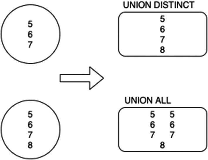
UNION ALL vs. DISTINCT
INTERSECT (DISTINCT)
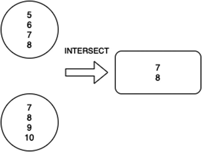
INTERSECTION
EXCEPT (DISTINCT)
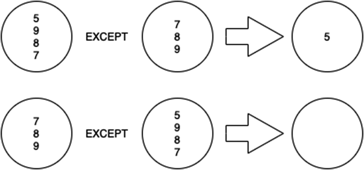
EXCEPT
Joining
Joining is the process of connecting two tables together by use of a common value. In data warehousing strategy, denormalization means that you limit the number of joins required to do a given operation. With BigQuery, the use of nested columns can limit the number of joins you must do to extract the desired data, even within the denormalized table structure.
In general and also for BigQuery, JOINs are not as performant as denormalized table structures. If you are finding that you are joining across large datasets as a matter of course and performance is degrading, this is an indication that your design needs adjustment.
(We won’t address if and how you should use joins in this section, only what they are and how they work.)
There are three basic types of joins: CROSS, INNER, and OUTER.
CROSS JOIN
Cross joins are much maligned because they simply calculate the Cartesian product of two tables and return everything. This can be a massively expensive operation, and should you do it without a WHERE clause, you will probably be visited by people in expensive black suits asking for “a word.” (Side project: What’s the most expensive single BigQuery call you could make that actually returns? It almost certainly involves cross joins.)
At least then, someone might catch it in code review and ask you what you are even doing there.
That being said, there are some valid use cases for the cross join. The best example is if you need to return data for every combination of certain variables. For instance, if you had ten data entry workers and you wanted to see how many records they had input in each one-hour period, you could cross join a list of the workers to a table containing the numbers (0..23), which would give you all workers and all hourly periods, to which you could then OUTER JOIN the data you need. This example is a stretch, since there’s a better way to do it in BigQuery using UNNESTing.
(That way is SELECT * FROM UNNEST(GENERATE_TIMESTAMP_ARRAY(...)).)
INNER JOIN
An INNER JOIN combines two tables on a common value. (It’s the same as A CROSS JOIN B WHERE A.column = B.column, if that helps.) You use this join type when you only want rows where the key appears in both tables.
Incidentally, you always need a join condition unless you’re doing a cross join (or an UNNEST). Otherwise, there’s no method the parser can use to determine which rows you want.
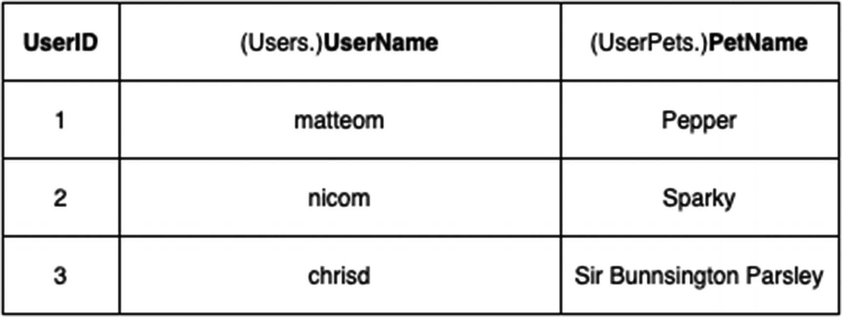
Inner join results diagram
We’ll revisit this in querying with nested columns in the following.
OUTER JOIN
OUTER JOINs often trip people up when they first encounter them. Think of an outer join as the following—no matter which option you choose, at least one of your tables will remain intact. Then, the other table will come along and attempt to match on the join condition. If it succeeds, the data will appear in those columns. If it fails, the row will remain, but its columns will be NULL.
For a LEFT OUTER JOIN, your first table remains intact. For a RIGHT OUTER JOIN, your second table remains intact. For a FULL OUTER JOIN, both tables remain intact.
(Using this model, an INNER JOIN is like mutually assured destruction. Two tables collide, and if they can’t find a match, they destroy the row.)
LEFT OUTER JOIN
In the LEFT OUTER JOIN, rows from the first table will always be retained, even if no data was found in the second table matching the join condition.
RIGHT OUTER JOIN
Amazingly, this is the opposite, where rows from the second table will always be retained, even if no data was found in the first table matching the join condition.
FULL OUTER JOIN
A full outer join is essentially doing a LEFT and a RIGHT outer join at the same time. All rows from both tables will be preserved, even if none of the rows matched the join condition.
This is not the same as a CROSS JOIN—a CROSS JOIN does a direct Cartesian product, which means that if one of the tables in a CROSS JOIN has zero row, you will get zero row. A FULL OUTER JOIN will instead return the schemas of both tables, but all the data on the side which was empty will be NULL.
USING
In the INNER JOIN form, the result set will return both A.x and B.x as columns. Since it’s an inner join, the columns will always have the same value. This often happens when you’re building an INNER JOIN query for the first time—you’d try to SELECT x, and it would give you an ambiguity error and require you specify whether you want A.x or B.x, even though you know they’re equivalent by query definition.
with no trouble at all. This is a nice bit of syntactic sugar that improves readability and avoids those ambiguous column errors.
Self-Joins
You can also join a table to itself. You would generally do this when you need to traverse some sort of hierarchy. Typically it means that there is a relationship modeled within the same table, as in an organization chart or a category tree. You want to get both the original record and its related record back in the same row.
There’s nothing inherently wrong with this, but in the same way that you want to model relationships with nested and repeated columns, you would want to do that here too. Yes, that means duplicating information in some columns in rows of the nested column. That is also a form of denormalization, and it’s worth considering here.
Subqueries
Subqueries comprise the intermediate results of a more complicated query. They’re useful when you need to do multiple steps of aggregation or transformation within the same query. In places where you only get a single statement context, like Dataflow SQL or a scheduled query, they allow you to do more.
However, once you begin using subqueries, your statements can start getting pretty complicated, so this is where you will want to begin focusing on readability. The easiest way to do this is to give your subqueries alias table names to indicate the intermediate step.
In this query, you use the subquery to make a table value called PetCount. Then, you can join that as if it were an actual table to the Users table and return all the users, their phone numbers, and the number of pets they have.
While extremely powerful, you can see how nesting several levels of subqueries could be very difficult to read. If you mix that in with BigQuery nesting and array syntax, you are creating a potential nightmare for others or future you.
WITH Clauses
This is slightly more readable, but as the number of subqueries grows, you will see increased benefit to this technique.
If you find yourself writing the same WITH clause over and over again at the top of each of your queries, it may be a good candidate for a denormalized table or a view.
Nested Data
So far we’ve stuck to concepts that are equally applicable to online transaction processing (OLTP) databases. And, as we’ve discussed, if you’re operating on small amounts of data, you may opt to retain some of the normalization and join syntax that you would use in the operational store. (As a reminder, BigQuery’s recommended threshold is that you can leave any dimension smaller than 10 GB normalized if you wish.)
At scale, your queries should definitely be minimizing joins and subqueries to achieve maximum performance. Google’s recommendation for BigQuery suggested nested and repeating columns wherever possible. Possible has a broad definition here; you don’t need to optimize anything until you start to see performance issues. As covered in previous chapters, many datasets won’t require any transformation at all to perform acceptably on BigQuery.
UNNEST
(I used the prefix DW, for “Data Warehouse,” to differentiate it from the earlier, normalized version of the table.)
This query will run faster and use substantially less data, since it doesn’t need to scan a second table at all. Note that there is no join condition here, since the nested column is already “joined” to the table.
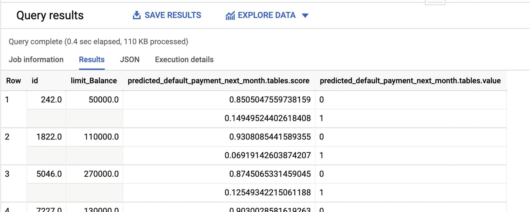
Console screenshot of nested table
This can get quite difficult to read and seems to be the biggest barrier for visual learners to jump in. You can explore these tables with UNNEST or with EXCEPT to exclude the record columns while you’re looking to understand the schema.
The reason this doesn’t work should make sense now; you can’t access a repeated field inside a table without flattening or aggregating it in some way.
If you’re still having trouble grasping this concept, I encourage you to get into the console and explore the syntax. Working fluidly with nested columns is a critical part of using BigQuery successfully.
Working with Partitions
Most of the loading and streaming options recommend or automatically generate partitioned tables. The primary purpose of partitioning is to reduce the number of partitions a given query needs to look at; this is known as partitioning pruning. When querying partitioned tables with BigQuery, your objective is, whenever possible, to look at the fewest number of partitions to retrieve your results.
Ingestion-time partitions
Date/timestamp partitions
Integer range partitions
Each of the three has slightly different ways of expressing queries.
Ingestion-Time Partitioned Tables
For these tables, which you created when you streamed data into the warehouse in Chapter 6, you don’t actually specify the partition column. It’s inferred and created automatically when the data is inserted into the table.
This is done by the creation of two “pseudocolumns” called _PARTITIONDATE and _PARTITIONTIME, which are reserved by BigQuery. In order to effectively prune partitions, you need to use these columns to filter the query to look at only the qualifying partitions.
This will throw out every partition except the one for that date. Be careful to avoid subqueries or functions that will make it impossible for the BigQuery parser to prune partitions.
Date/Timestamp Partitioned Tables
One way to know that you’re hitting the partition is that BigQuery can detect partitions as part of its estimate. There was a time when it did not do this, and it was scary for everyone, but now you can be sure before you start. In this case, the preceding query accesses only 6.1 MB. Without a partition filter, it would access a whopping 9.5 GB. So it makes a huge difference.
However, be sure to avoid subqueries or complex WHERE conditions when seeking to filter. BigQuery can only prune partitions if the query doesn’t need to look outside of your requested partitions in order to satisfy the WHERE clause. In the preceding example, no math or extra calculation is done on the TIMESTAMP. You may want to experiment a bit, since BigQuery’s partition optimization ability seems to be steadily improving.
You can also set a rule on a table you created this way that queries must specify a partition filter to execute. This rule is called “Require partition filter,” and it can save you a lot of money if you have analysts who have a tendency to use a lot of *s.
If you only need to access a single partition, and you know which one it is, you can use the $ syntax to reach it. For example, SELECTing from a date-partitioned table called DatePartitionedTable$20200101 would go directly to the underlying partition for that date.
Integer Partitioned Tables
Integer partitioned tables behave basically the same way as date-partitioned tables, except that the query in question is a number. As long as you perform a WHERE clause on the partition key and don’t perform any calculations or subqueries using it, the partitions will automatically be used.
Also as with the date-partitioned tables, you can go directly to an underlying partition by using the $ syntax, that is, IntegerPartitionedTable$100.
Date, Time, and Timestamp Functions
DATE
DATETIME
TIME
TIMESTAMP
Of the four, only TIMESTAMP represents an absolute point in time. The other three represent what I’ve been calling “local time” and Google calls “civil time,” namely, a timezone-independent representation of a logical date and/or time.
This can be pretty hard to grasp when you’re dealing with events. I find it easiest to think of it in terms of which context is relevant: the record’s or the absolute time. Let’s look at an easy example: January 1, 2001, at midnight, otherwise known as the beginning of the current millennium.
Cities who shared a timezone with UTC, like London, were indeed singing “Auld Lang Syne”. But in Chicago, the clock said 6 PM on December 31st. So which time matters? The answer is the same as the answer for whether you are thinking about a TIMESTAMP or a DATE/DATETIME/TIME. A TIMESTAMP occurs at the same microsecond everywhere. (No letters about relativity, please.) A DATE represents an arbitrary period where the calendar had that value on any particular date.
Coordinated Universal Time (UTC)
Use UTC whenever possible in storage. This allows you to do date math without trying to account for timezones, and it also allows for the very common pattern where a user in a certain timezone would like to see the results as local to them. For example, if someone logged in at 5:36 PM Pacific Standard Time and I’m looking at an event log while in Eastern Standard Time, I’d like to see that the event occurred at 8:36 PM “my” time. Storing the event at the absolute UTC timestamp would allow you to perform that conversion without manual error.
I’m not going to sugarcoat it; managing time data is one of those things that seems like it should be really easy until you actually start to get into globally distributed systems. Basic assumptions don’t hold true—you can’t actually calculate the distance between the current time and a UTC timestamp in the future, because leap seconds may occur. And ultimately because time is a human construct and we’re modeling a physical process, that is, the rotation and orbit of the Earth, there will always be discontinuities. Luckily, as long as you stick with UTC, pretty much all of them will be at a higher level of precision than we care about .
Common Use Cases
Let’s briefly cover each of the data types and their precisions. After that, we’ll look at some of the functions and their common uses. The majority of functions have a suffix for each data type. For example, CURRENT_TIMESTAMP, CURRENT_DATE, CURRENT_TIME, and CURRENT_DATETIME are all valid. For further reference, the BigQuery documentation on these functions is quite good.2
DATE
DATE takes the form YYYY-[M]M-[D]D and as such has a maximum precision of one day. The valid range is from 0000-01-01 to 9999-12-31, so if you want to represent the ancient Egyptians or the Morlocks, you’re out of luck.
TIME
TIME has microsecond precision and a form of [H]H:[M]M:[S]S[.DDDDDD]. You can go from 00:00:00.000000 to 23:59:59.999999, which means no Martian time here.
DATETIME
As a logical combination of the preceding two types, the DATETIME object ranges from 0000-01-01 00:00:00.000000 to 9999-12-31 23:59.999999. This gives you the full range of precision from year to microsecond. The canonical form is a DATE plus a TIME, with either a “T” or a space between them.
TIMESTAMP
As mentioned earlier, the TIMESTAMP is the only data type of the four that represents a fixed, absolute point in time. This adds one more value, which is the timezone. The default is UTC, but you can also represent absolute timestamps in other timezones. This means that the same canonical form of DATETIME can be accepted for a TIMESTAMP, but you can also append the timezone code at the end.
Note that BigQuery doesn’t actually store the timezone—it doesn’t need to. Each timezone has its own representation of the UTC fixed time. You use timezones when searching or inserting and to format the value for display; the internal value doesn’t change.
You can represent a timezone either with a “Z” (Zulu) to explicitly indicate UTC or by specifying the name or offset.3
Date Parts
MICROSECOND
MILLISECOND
SECOND
MINUTE
HOUR
DAY
WEEK
WEEK([SUNDAY, MONDAY, TUESDAY… SATURDAY])
MONTH
QUARTER
YEAR
MONTH and YEAR also have ISO variants using weeks as defined by ISO 8601 .
Intervals
In order to work with lengths of time, you need to declare an interval. An interval consists of an integer combined with a date_part, like (INTERVAL 5 MINUTES) or (INTERVAL 13 DAY). The construct has no use by itself; you must use it in combination with one of the date functions. Note that the numeric part must be an integer. You can’t add 1.5 YEAR or 0.25 HOUR.
CURRENT
CURRENT_(TIMESTAMP/TIME/DATE/DATETIME) will return the current date and/or time.
_ADD, _SUB, _DIFF
These three functions exist across all four data types (i.e., DATE_ADD, TIMESTAMP_DIFF, TIME_SUB, etc.).
You use them to add or subtract an interval to and from a datetime or to find the distance between two datetimes using a given date part.
_TRUNC
DATE_TRUNC, TIME_TRUNC, DATETIME_TRUNC, and TIMESTAMP_TRUNC allow you to quantize an object to a lower level of precision. For example, you can use DATE_TRUNC(DATE ‘2001-01-13’, MONTH) to truncate to month-level precision, 2001-01-01.
EXTRACT
Again, if you specify a date_part that isn’t part of that data type’s precision, it will fail with an error message like “EXTRACT from TIME does not support the YEAR date part.”
Formatting and Parsing
A number of the other date functions convert between string-based values and date/time objects or vice versa. When dealing with data from external data sources, you will frequently need some conversion to deal with another system’s data formats. You can use ISO date specifications as a common format. Watch out for timezones!
UNIX Epoch Operations
When dealing with UNIX-based external systems or older timestamp systems, you will often encounter the concept of the epoch. This is the amount of time that has passed since UNIX’s arbitrary second 0 on 1970-01-01T00:00:00Z. You can use UNIX_SECONDS, UNIX_MILLIS, or UNIX_MICROS to get the current epoch date for a given timestamp. To go the other direction, you can use TIMESTAMP_SECONDS, TIMESTAMP_MILLIS, or TIMESTAMP_MICROS.
The epoch format has three levels of precision, which depend on your use case. The original UNIX version used only second-level precision. Javascript’s underlying support uses millisecond-level precision. Systems analysis, performance counters, and the global positioning system (GPS) itself have microsecond resolution.
Grouping Operations
Earlier in the chapter, we explored basic grouping. There are more things we can do with grouping, and it is important for dealing with large datasets to return data in the buckets that we need.
Much like ordering, there are also data types that do not support grouping, and they’re the same data types: ARRAY, STRUCT, and GEOGRAPHY. You can also use integers positionally in GROUP BY clauses as with ordering (i.e., GROUP BY 1), but I also discourage their use for similar reasons (in a word, brittleness.)
ROLLUP
Using the rollup keyword allows you to use grouping “sets,” instead of grouping by only the one grouping set defined in the initial GROUP BY. To do this, it multiplies the GROUP BY set into its constituent subsets and then unions them together.
Effectively, this gives you multiple levels of GROUP BY without having to specify the grouping sets directly. For rows representing a “rollup,” the grouping key will be null.
This concept can be a little weird to understand at first; I usually use the concept of budgeting to explain it. Suppose your organization has three departments: accounting, HR, and executive. (This company obviously doesn’t do anything.) Each of those departments has individual expenditures, and you want to see the amount of money they have each spent.
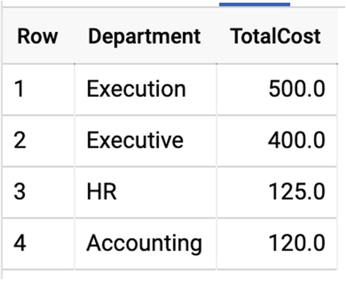
Result table
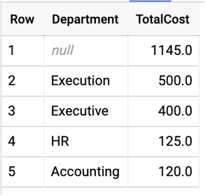
Result table with null row
That NULL row represents the SUM applied to the individual buckets’ sums.
HAVING
The HAVING keyword is much like WHERE, except that it follows GROUP BY in the order of operations. This keyword lets you filter the results of a GROUP BY for additional conditions.
After the GROUP BY is applied, the HAVING clause filters its rows to just those that qualify. Note that aggregation is present both in the SELECT and the HAVING, but you could also filter by rows HAVING AVG(Cost) > 50, for example, to only return departments whose average expenditure exceeded $50.
Aggregation
As a related item to grouping, we also looked at some common aggregate functions earlier in the chapter. In addition to those (MAX, MIN, SUM, AVG, and COUNT), let’s look at the others. You can find dizzyingly comprehensive documentation for every type of function in the BigQuery documentation. (For reference, I’m repeating the preceding five as well.)
ANY_VALUE
Sometimes, you just need a representative value from the bucket, and it doesn’t matter which one. In that case, there’s ANY_VALUE, which non-deterministically pulls one qualifying value for the group and returns it to you.
You can also use MIN or MAX in any of these cases, but ANY_VALUE is faster, since it doesn’t have to do a sort.
ARRAY_AGG
ARRAY_AGG takes any value (except an ARRAY) and converts it into an array. It can handle values with multiple columns too, which means you can use it as a sort of opposite to UNNEST.
Even better, in combination with user-defined functions, which we’ll get to later, you can actually define your own aggregate functions that use ARRAY_AGG to filter elements in a way that you choose.
ARRAY_CONCAT_AGG
This aggregation only takes ARRAYs and creates the concatenated array containing all of the subelements. For example, if you had three rows, { [1, 2, 3], [4, 5], [6] }, running ARRAY_CONCAT_AGG on these values would generate a single array, [1, 2, 3, 4, 5, 6]. You can also specify an ORDER BY on the array concatenation, and you can LIMIT the number of arrays you will allow to be concatenated to a constant integer.
AVG
Returns the average value across all the rows in the group. This only works on numeric types, so don’t expect to average some strings together. (Yes, yes, I know you think the average of {“A”, “B”, and “C”} should be “B”. I just told you you can use ARRAY_AGG to write your own aggregate functions, so go ahead and implement it yourself.)
COUNT
Returns the number of rows in the group.
COUNTIF
will give me the number of expenses by department, but only where the expense was greater than $25. (WHERE HasReceipt = 0 would give me a list of offenders who didn’t submit expense reports that were over the $25 limit!)
MAX/MIN
As discussed before, returns the maximum or minimum value for that group.
STRING_AGG
STRING_AGG takes a series of values and concatenates them together into a single STRING (or BYTES) value. This handles the very common case that you have finished operating on the individual values and need to return or display them in a readable format.
SUM
The IF function evaluates the expression in the first argument and produces the second expression if true and the third if false. (Programmers recognize this as equivalent to ternary operator expressions like (sum > 150 ? cost : 0)). If the cost is greater than $150, the cost is supplied to the sum; if not, 0 is supplied, effectively skipping the row.
Bitwise Aggregation
Using the INT64 type, you can use BIT_AND, BIT_OR, and BIT_XOR to perform bitwise operations across values. (To specify hexadecimal values in BigQuery, use the form 0x0000.) LOGICAL_AND and LOGICAL_OR are similar, but operate on boolean values.
In databases where space was a constraint, data engineers would use packed fields to fit multiple values into a single column. For example, using an INT64, you could store 64 individual bits of data, that is, 64 boolean columns. To retrieve individual values, you’d first need to know which bit held the flag you wanted, and you would then apply a bit mask to get the value out.
These operators are still useful for manipulating columns that have been stored in this way, especially if you are transforming them into proper columns or arrays upon load.
BigQuery GIS
Geospatial calculations are a fundamental part of most data warehouses. Most businesses have the need to track what location things are in, whether it be consumer goods, vehicles, store locations, and so on. Being able to pinpoint something in time and space is a basic feature of much data analysis.
The BigQuery feature supporting geospatial data is called BigQuery GIS, or just GIS. Like most SQL geography packages, it has a series of common functions and operators designed to make it easy for you to do work with spatial coordinates and bounding boxes—no trigonometry required.
For the purposes of this book, BigQuery, and anyone outside of a space agency, we are using the WGS84 coordinate reference system, which takes the Earth to be an oblate spheroid 6378.1… No, sorry, geodesists. For everyone else, we’re using the longitude/latitude system to establish locations on the face of the planet.
If you weren’t paying attention in geography class, crash course. Latitude can go from +90 degrees (90°N, the North Pole) to -90 degrees (90°S, the South Pole). Longitude goes from -180 longitude (180°W) to +180 longitude (180°E). -180 and +180 degrees of longitude represent the same meridian, the farthest away from 0° longitude, which is almost at the site of the Royal Observatory Greenwich in London, United Kingdom, but not quite. Using this system, you can specify any location on Earth to an arbitrary degree of precision. The history of coordinates is incredibly fascinating and almost entirely irrelevant to BigQuery, other than at this one intersection point.
The breadth of this issue is enormous, and a full treatment would deserve a book of its own. But you will almost certainly encounter use cases requiring it, and there’s no need to subject yourself to the pain of trying to manage a separate latitude and longitude column in all of your tables. If working with the GEOGRAPHY type seems natural to you, you will be able to do all kinds of fascinating analysis.
There’s only one data type in play here: GEOGRAPHY. But the GEOGRAPHY type is pretty complex, so we’ll break it down.
GEOGRAPHY Concepts
Point
The simplest unit of location is a point. A point can be constructed with just the latitude and longitude, which uses the ST_GEOGPOINT function to yield a GEOGRAPHY type.
Line
A line is the shortest distance between two points. Using ST_MAKELINE, you can take two or more points (or lines) and join them together to make a single, one-dimensional path called a linestring.
Polygon
A polygon is a geography consisting of multiple linestrings. To form a polygon, you must have at least three linestrings where the first point of the first linestring and the last point of the last linestring are exactly the same point. That is, to form a valid polygon, you have to end where you started. Then, you use the ST_MAKEPOLYGON function to generate the GEOGRAPHY which contains the surface area.
Because the Earth is round (seriously, no letters) and thus the coordinate system is contiguous, any given polygon specifies two surface areas—what’s inside it and what’s outside it. Think about it—if I draw a square on a globe, am I enclosing the space inside it or outside it? By convention and common sense, the ST_MAKEPOLYGON function defines the space to be the smaller of the two options; so, if you draw a polygon around the state of Wyoming, MAKEPOLYGON will create the geography of the inside of the state, as opposed to the geography of everything outside the state. You can change this behavior with the ST_MAKEPOLYGONORIENTED function.
GIS Functions
Whew. Let’s skip ahead and say you’ve just inherited some GEOGRAPHY data. Honestly, this is probably exactly what will happen. You don’t generally need to define your own GEOGRAPHYs; they usually come prepackaged from other data libraries. For example, if you go to www.arcgis.com, you can download datasets that represent the boundaries of common geographical objects like states, rivers, streams, and so on. Luckily, the work of centuries of surveying has given us extremely accurate representations of the world we live in. (Well, reasonably accurate. The state of Colorado, despite its appearance on a map, is a polygon containing hundreds of sides. And did I mention US zip codes have no canonical polygonal representation at all? But…when you use a store locator… Not now.)
Assuming you have some GEOGRAPHY objects lying around now (Chapter 20 has some too), let’s look at a sampling of the functions we can use on them. Note that since a GEOGRAPHY may contain one or more polygons, lines, or points, functions are not always applicable to a given value of the data type.
ST_DIMENSION
I include this one so you can get a sense of your bearing when first looking at GEOGRAPHY objects. ST_DIMENSION(geography) will return 0, 1, or 2, indicating whether the highest-order element in the input is a point, line, or polygon, respectively. (Empty geographies return -1.)
ST_AREA
This function works on one or more polygons to tell you the total surface area covered in square meters. The area of a line or point is 0.
ST_CENTROID
This function will return the centroid of all of the elements in the geography, using the function for the highest dimension available. A centroid, in basic terms, is the “center” of a group of points, lines, or polygons. The math can get fairly complicated in higher dimensions, but in practical terms, this tells you where you might center your map to visualize all the values inside. (You can also then apply ST_MAXDISTANCE to figure out the zoom level for that map.)
ST_DISTANCE
ST_DISTANCE gives you the shortest possible distance between two GEOGRAPHY objects in meters.
ST_LENGTH
ST_LENGTH operates on lines to return the total length of all lines in the GEOGRAPHY in meters. If the GEOGRAPHY contains only points or polygons, the result is 0.
ST_X/ST_Y
ST_X and ST_Y are how you take a single point and break it back out into its longitude (ST_X) and its latitude (ST_Y). You will have to do this for any external system to plot points on a map; for example, if you pull ST_X and ST_Y for any GEOGRAPHY point, you can pop them into Google Maps with (www.google.com/maps/place/) [ST_X],[ST_Y] and see that point on the map.
Other Functions
The other geographic functions allow you to do things like see if GEOGRAPHY objects cover each other’s area, if they intersect at all, or if they touch, perimeters, boundaries, and a whole set of conversion functions from other common geography data representations.
Joins
You can use some of these functions as join predicates too. For example, you could write a query to join a list of service areas with a list of state areas on whether their geographies intersect: this would tell you which states had any service areas. You could then use a GROUP BY to SUM the ST_AREAs of each of the service areas to figure out what portion of the state’s area was covered by your service areas.
With a little extension, you could easily discover which metropolitan areas are covered by the fewest zip codes. By simply removing the WHERE clause, you can learn that the zip code 99752 is actually 4,000 times larger than its designated metro area of Kotzebue, Alaska.4
Visualization
Dealing with arbitrary locations in numerical form can be aggravating. Sometimes you just want to see what you’re dealing with on a map.
There are several options available, including Google Earth Engine, but we’ll focus on the simplest in order to help you understand and work better with your geographic data. That’s BigQuery Geo Viz, located at https://bigquerygeoviz.appspot.com/. I found this tool to be invaluable when learning about geographic data types.
Authorize the site to access your BigQuery instance, and your project IDs will populate in step 1. Select the project you’re using, and type in a query which returns a GEOGRAPHY result in a column. The map will automatically visualize all of the points for you. You can click each point to see the rest of the row for that location.
This tool is not really intended for production use. You can’t share or download maps. But it gives you an easy, valuable visualization directly out of BigQuery. I hope that they incorporate it directly into the query results at a future date.
Other Functions
Frankly, the SQL standard is massive; and even with a broad survey, we haven’t even scratched the surface. There are hundreds of other functions for string manipulation, math, networking, and encryption. Google’s documentation is excellent on these points, and you can read it here (https://cloud.google.com/bigquery/docs/reference/standard-sql/functions-and-operators).
Suffice it to say, if you need to do data transformation using only SQL statements, you’re still well-covered.
Summary
SQL is a huge language, and thousands of books have been written just about writing effective queries. BigQuery is SQL-compliant, so all of that power is available to you in your data warehouse too. Retrieving data from a database always follows the SELECT/FROM/WHERE pattern at heart. You can also join tables together, or you can use nested and repeated columns to avoid them. SQL offers a variety of functions for date math, aggregation, field manipulation of all kinds, and geospatial support. Even that barely begins to tell the story; there are hundreds of other functions available.
Before returning to SQL, we’re going to diverge in the next few chapters to explore some other GCP services that work well in tandem with BigQuery to solve common problems. First up is how to schedule queries and jobs so that you can run operations inside BigQuery on a prescheduled or recurring basis.