Once you have your data warehouse built, its schemas defined, and all of your external and internal data migrated into BigQuery, it’s time to start thinking about your data pipeline architecture and how you can enable your organization to accept stream or batch processing into the warehouse.
Your organization may already have a well-established system of relational or NoSQL databases collecting and distributing data to end users. The trick is to get that data into BigQuery as efficiently as possible so you can begin analysis. If your organization has or requires big data pipelines, at some point you are going to hit a limit that might be bounded either by scale or by the amount of time you have to devote to the problem.
When you reach this point, there are still plenty of options—you could employ a custom architecture using functions as a service (FaaS), or you could use any of the available transfer mechanisms through the native features of your SQL or NoSQL platforms. You might even rely on some of the basic methods we discussed in earlier chapters, like maintaining read-only replicas or streaming data directly from sources.
However, at massive scale, it becomes difficult to keep track of your data configurations. With manifold data sources and disparate transforms, an organization can become quickly overwhelmed with preprocessing raw data to do analysis. Dumping your data rapidly into lenient BigQuery schemas and crunching it later can become the equivalent of shoving all your dirty laundry into a closet. While efficiently dealing with a problem at the beginning, you pay for it later in the amount of time required to retrieve and organize the data (or socks). This is not an ideal system of prioritization for data at scale.
Enter Google Dataflow. Dataflow is Google’s managed service for processing and transformation. Like most of the other Google Cloud Platform (GCP) products in this book, it uses a serverless model and is designed to abstract the challenging management of concurrency and parallelization so you can focus purely on what you want to do with the data.
Google Dataflow was originally developed at Google (“Dataflow Model”) and intended as a successor to technologies like Apache Hadoop MapReduce and Apache Spark. In 2016, Google joined a group of other developers with a proposal to open source the Dataflow Java SDK as an Apache Software Foundation incubator project. When the SDK was open sourced, it took the name Beam, a portmanteau of “batch” and “stream.” Google’s Java Dataflow SDK retained compatibility with Beam. In 2016, Google added Python support and, very recently and most excitingly, Dataflow SQL. The Dataflow SDK is also being deprecated and will use the open source Beam SDK. All this to say, you will see both Dataflow and Beam, and while they are not equivalent, they are closely related.
The development of Dataflow SQL and its underlying Apache Beam work is fascinating because it seems like an obvious choice, and yet Java and Python (and Go) appeared on the scene first. However, at the dawn of big data, when Hadoop and other map-reduce technologies were becoming popular, that was all that was out there. This has some pretty deep historical precedent. Björn Rost, the technical consultant on this book, surmises that this could be partially because SQL was designed originally for fixed storage, as opposed to streaming datasets. Streaming was also something organizations tended to do in a few isolated use cases. And yes, if you think about the world of RDBMS and how query engines were constructed, it made sense at that time to do certain data processing in procedural languages, outside the database. This was also convenient for software engineers, who were often nervous about SQL and considered query optimization to be a black art. (Those who embraced SQL also found welcome parallels in functional programming techniques and happily adopted relational algebra all over the place.) The merging of these two streams (no pun intended) is fairly recent, starting around when Kafka released KSQL (now ksqlDB). Both ksqlDB and Dataflow have had to contend that SQL is not built for streaming operations and have introduced extensions to compensate.
In the last several years, technologies like Google BigQuery, Amazon Redshift, and Azure Synapse Analytics have allowed SQL to regain its throne as a language at the terabyte and petabyte scale. As a long-time practitioner and admirer of SQL, I couldn’t be happier. Colonizing the entire data ecosystem with SQL feels like it was the natural choice from the start. And finally, the technology is catching up.
(Side note: Engineer-adjacent professionals like product managers and sales architects often ask me if they should learn to code. Whatever my specific answer is, I seem to always find myself veering into the recommendation to learn SQL. I really do believe that it changes your perception of how the world’s information is organized. Of course, you already know this.)
Key Concepts
Since Dataflow emerges from a map-reduce school of thought, its model resembles more of a phased workflow. Understanding the model and execution phases will help you design pipelines that best suit your needs.
Driver Program
The driver program, or just driver, is the execution unit that constructs the pipeline. In Java and Python, it is the actual executing program that instantiates the pipeline, supplies all the necessary steps, and then executes on an Apache Beam runner, in this case, Google Dataflow. In Dataflow SQL, this actually gets all abstracted away, but we’ll get to that later. Essentially, just be aware that if you are working with a procedural SDK like Java or Python, you’ll actually be writing the program to contain the job. (There are plenty of templates to assist with all kinds of common tasks.)
Pipeline
The primary object in Dataflow is the pipeline. The pipeline runs from start to finish and governs all the aspects of your task. Your ultimate deployment unit to manage Dataflow jobs is this pipeline. Beam drivers must implement a pipeline in order to do anything. The pipeline will in turn be responsible for creating the datasets (PCollections) that will be loaded and transformed throughout the life of the job.
The job is intended to represent a single workflow and to be repeatable. Thus, it can both be parallelized and run continuously inside a Beam-compatible framework like Google Dataflow. Under the hood, a Beam pipeline looks a lot like something you would see in Apache Spark or really any other workflow tool: a directed-acyclic graph (DAG).
Directed-Acyclic Graphs
If you’re at all familiar with graph theory, skip this section.
Directed-acyclic graphs , or DAGs, come up theoretically as great interview questions in a wide variety of mathematics and computer science subdomains. They tend to pop up anywhere you want to understand or generate a static graph of an execution flow, in compilers, and so on. If they’re not interesting to you in this context, they’ll probably surface somewhere else.
“Pipeline” is an evocative term that summons large industry to mind. It also implies a straight line from input to output, and in some ways it doesn’t really touch on the importance of data transformation in the process. The reality of a workflow-based structure is slightly more complex. As far as your business owners are concerned, expressing data processing as a series of tubes is a perfectly fine approximation, but as you come to work with the technology, it’s useful to go one level deeper.
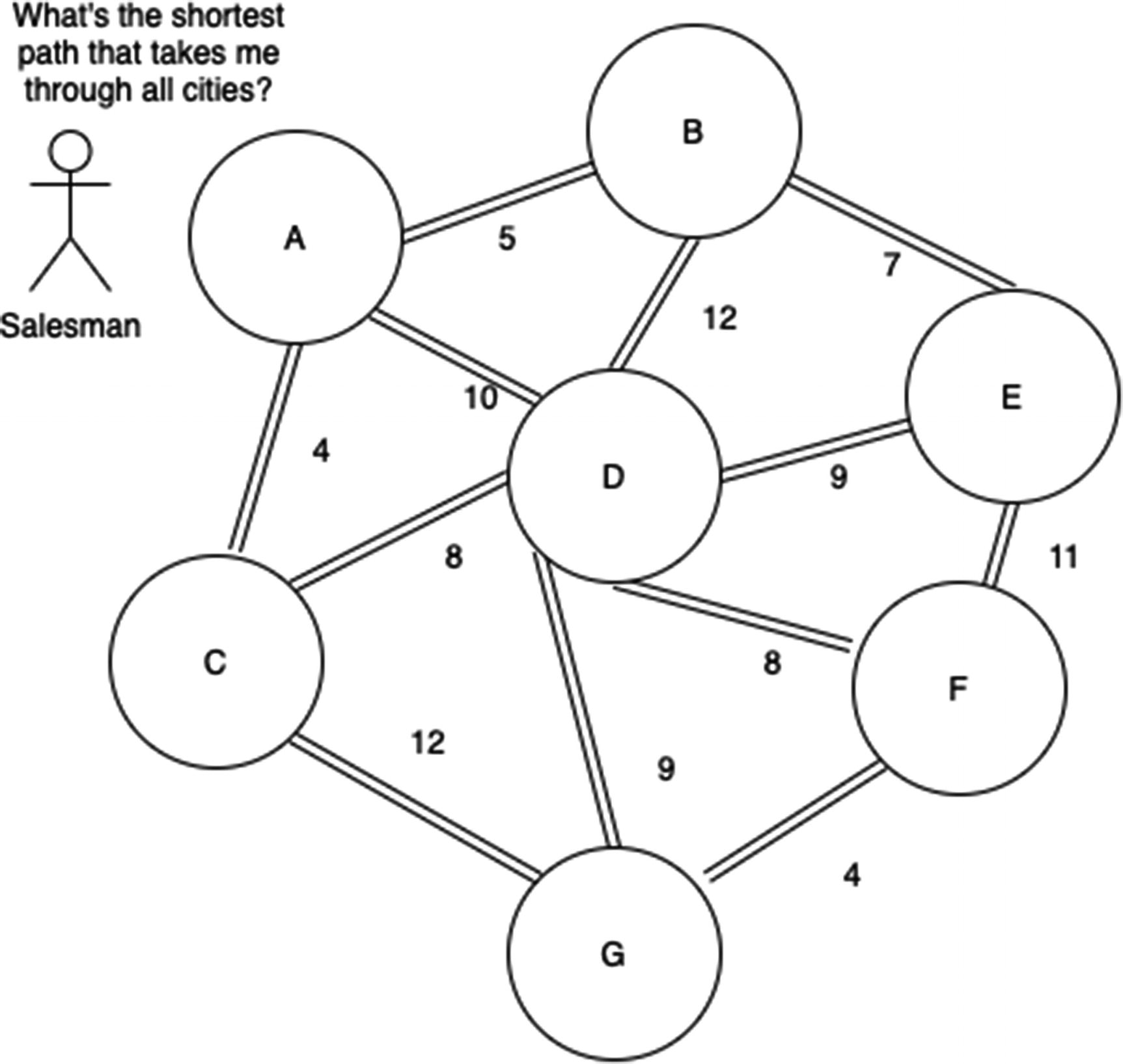
a graph as might be seen in the Traveling Salesman Problem
Directed: This means that the edges between nodes have a direction, typically represented with an arrow. You may only proceed along edges in a valid direction.
- Acyclic: This means that there are no “cycles” in the graph, meaning that you can never start at one node and, following the arrows, end up back at that same node. This should be a familiar programming concept—a cycle connotes an infinite loop. Infinite loops in tasks that are supposed to complete are bad!
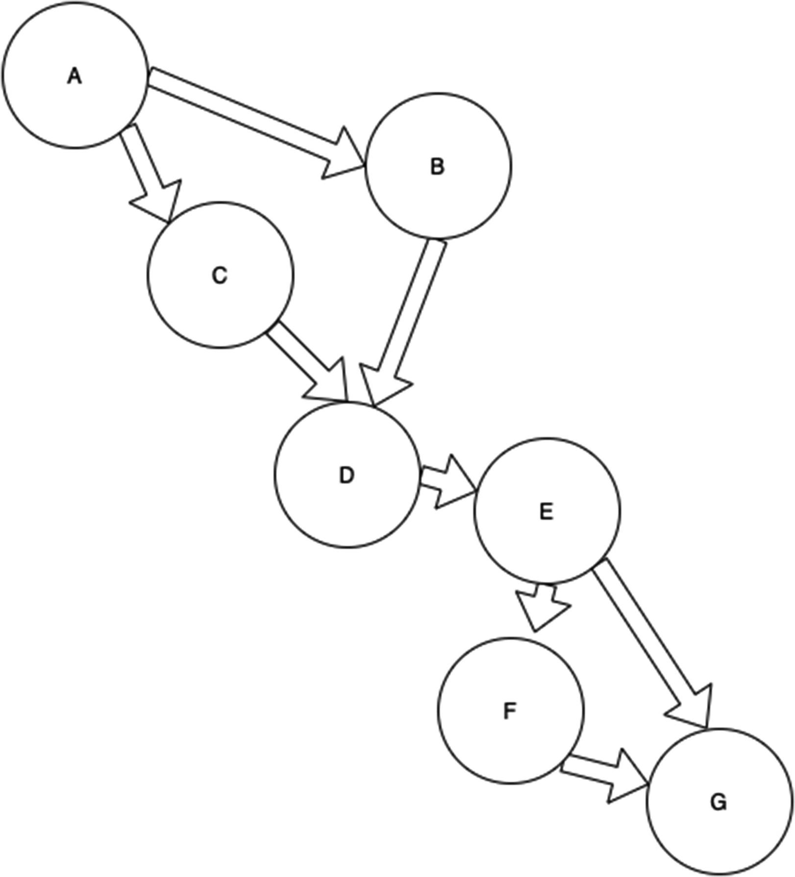 Figure 7-2
a directed acyclic graph
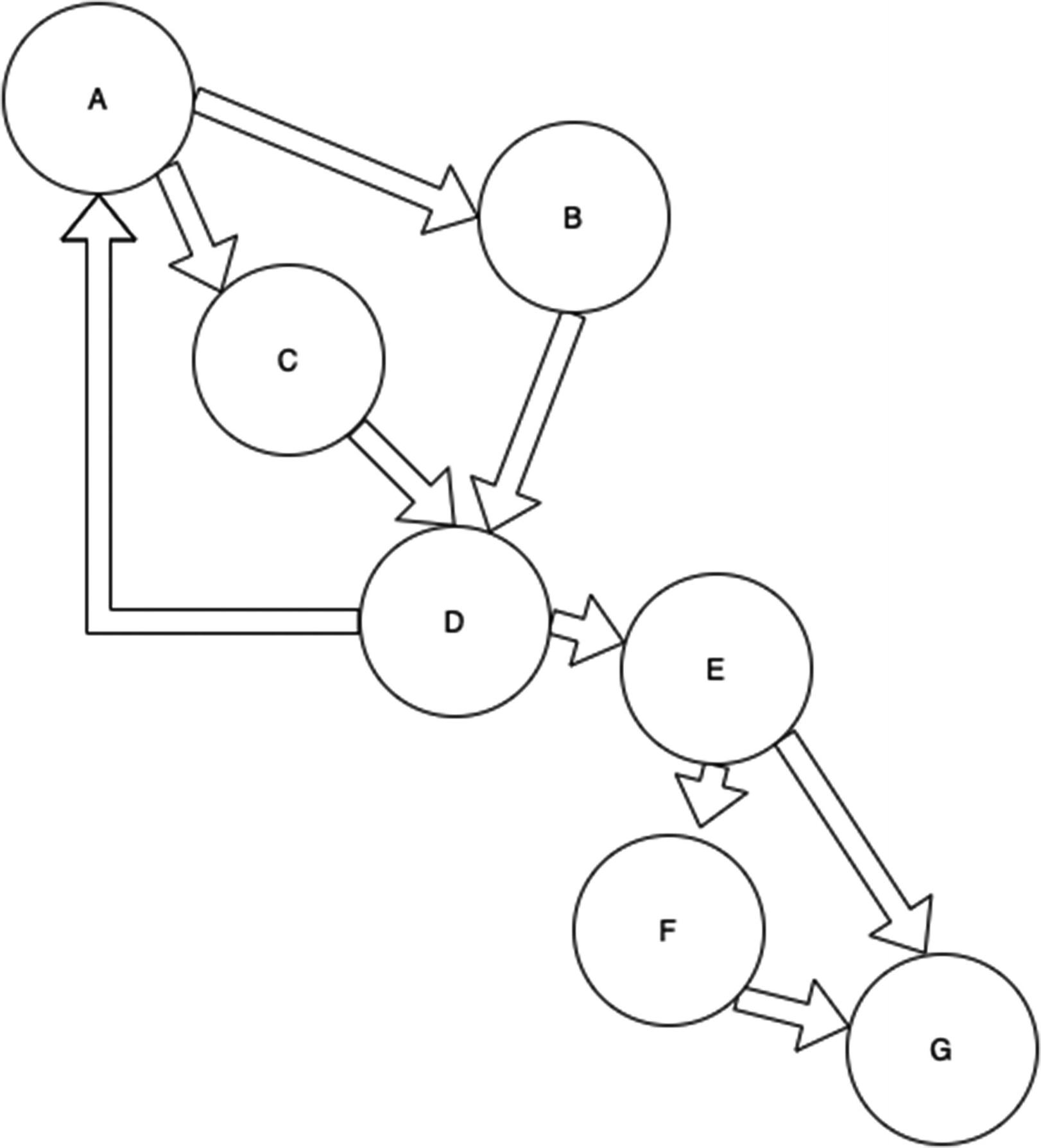 Figure 7-3
a graph with directed cycles
There’s usually one additional restriction for workflows that operate using a DAG, while not part of the formal definition. Usually disconnected nodes aren’t permitted—that is, every step in the workflow has to be reachable. It doesn’t really make sense to write steps that can’t be executed.
With the difference between the admittedly friendlier term pipeline and a directed-acyclic graph, thinking about this in terms of graph theory may assist you in quickly distinguishing between valid and invalid workflows.
PCollection
A PCollection is the input and output object for the pipeline’s steps (graph vertices). The whole pipeline will start by initializing a PCollection. That PCollection will represent the dataset, which comes from a bounded (like a file) or an unbounded (like a stream) data source. This also helps establish the basis for a job that will run on finite input files or for one that will run continuously hooked up to a queue. This data source is generally also provided from a location external to the pipeline’s starting point.
Technically, you can initialize a starting PCollection with values internal to your driver program as well. This could be a handy use case if the primary concept you need to transform is a fixed list of data, and you’re going to be collecting auxiliary data to join from the external source.
In general, however, I would encourage you to think of the pipeline as being controlled by the input data. Thinking about the pipeline in terms of widest to narrowest will create the highest degree of parallelization and avoid the bottlenecking that might be caused by running a small dataset over and over again and trying to join it up to larger sets.
(A job that only looks at internal data may be fast and repeatable, but it won’t accomplish anything useful. If that’s what you are hoping to do, you can probably get the same result by running a BigQuery query by itself. Techniques in earlier chapters would probably suffice without the cost and effort of following the data flow path.)
Each PCollection’s elements get assigned a timestamp from the source. (Bounded collections all get the same timestamp, since they aren’t continuously streaming.) This will be important as it drives the concept of windowing, which is how Dataflow is able to join datasets when it doesn’t definitively have all of the data for any of them, except again in the case of bounded sets.
Another important note: PCollections are immutable. One of the key properties of the Beam model is that you must not modify the elements of a PCollection that you are processing. This is a familiar concept in functional programming models, but the underlying reason is because parallelization doesn’t work if objects can change unpredictably. A given PCollection may undergo multiple transforms in a non-deterministic order of execution. If any of the relevant transforms modify the object, all the others will get a different copy, which will yield different results.
This could happen easily with branched transforms, where you send the same PCollection to multiple PTransforms for different purposes. For instance, say you have a bounded dataset with the numbers 1…100. Transform F should filter all the numbers divisible by 3, and Transform B should filter all the numbers divisible by 5. Let’s say that one of those transforms removes the number 15 from the PCollection, which is applicable to both filters. This means that the order of execution will now determine how one of the transforms operates. One transform will see the number 15, and the other will not. The results will become only more unpredictable and distorted as future PTransforms try to operate on disjoint datasets. The Java SDK will detect and reject transforms that modify PCollections, but if you find yourself running into this issue, remember that parallelization is dependent on consistent data.
PTransform
A PTransform is the actual step in the pipeline, which takes one or more PCollections as input and returns zero or one PCollection as output.
Thinking about it from a graph perspective, this means that instances of the PTransform object each do the work from beginning to end, by passing PCollections around. A PTransform object might take multiple PCollections as input because it needs to join or filter them. However, it can only produce one PCollection as output because it should only have a single responsibility, to do something with the data and output a dataset (PCollection) that’s slightly closer to the final form you are looking for.
When a PTransform outputs zero PCollection, that’s the end of that particular journey. Note that you could have several destinations in your pipeline that output zero PCollection if you are writing to different places or writing different kinds of data. (Directed-acyclic graphs don’t mandate that there only be a single termination point to the graph.)
Applying a Transform
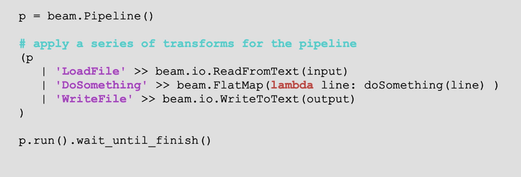
code example to show application of transformation
Basic Transforms
ParDo: From “parallel do,” this is the generic parallelization method. To use it, you create a subclass of DoFn and pass it to the ParDo.
GroupByKey: This transform operates on key-value pairs. Much like SQL GROUP BY, it takes a list of elements where the key is repeated and collapses them into a PCollection where each key appears only once.
CoGroupByKey: This transformation operates on two or more sets of key-value pairs, returning a list of elements where each key in any of the datasets appears only once. This is somewhat like doing a UNION of the same primary key on multiple tables and then using a LEFT OUTER JOIN on all of them to retrieve the distinct data for each key. A key only needs to appear in a single input dataset to appear in the output.
Combine: This is actually a set of transforms. You can take action to combine all elements in PCollections, or you can take action which combines across each key in a set of PCollections with key-value pairs. You can also create a subclass of CombineFn and pass it to Combine to perform more advanced operations.
Flatten: This is much like a SQL UNION ALL operation in that it takes multiple PCollections and returns a single PCollection of all of the elements in the input collections. You’re most likely to see this approaching the end of a pipeline, when eligible data has been through several separate branches of transformation and is getting prepped for writing.
Partition: This transform takes one PCollection and, using a subclass of PartitionFn that you define, splits it up into multiple PCollections stored in the form of a PCollectionList<>. This partitioning cannot be dynamic, which I’ll cover in the following.
Learning about these transforms may have raised a couple of questions with respect to how Dataflow will actually work. Before we get into the actual nuts and bolts of building a pipeline, let’s address a couple of them.
Firstly, some of these operations appear to work like joins or aggregations. But how can those operations work if the full content of a dataset is unknown, as it definitionally is for streams? The answer is windowing: Dataflow needs to either be able to estimate when the dataset has been delivered, or it needs to break the datasets up into time-based windows. Remember from earlier when I said that PCollection elements all get a timestamp? That’s what this is for. Advanced windowing is quite complicated. We’ll discuss it in Dataflow SQL, but for now remember that we’re not operating with fully materialized datasets here. Each dataset must be divided in some way. Furthermore, if you try to perform a combine operation on two datasets that don’t have compatible windows, you won’t be able to build the pipeline. This is critically important in both the Java/Python and the SQL flavors of Dataflow.
Secondly, as to why partitioning cannot be dynamic, the workflow graph must be constructable at runtime. You can’t do anything once the workflow is running to change the number or order of steps. This is often cited as a weakness of the Apache Beam model, and there are certainly data processing scenarios where it could pose a problem for you. It is definitely something to keep in mind as a limitation of the system as you proceed.
Building a Pipeline
So now you have a good idea of all of the basic elements of the pipeline and what kinds of operations are possible. Everything up until this point is common to Apache Beam, but from this point, we’ll jump into Google Dataflow and use practical examples.
a simple Pipeline
a complicated Pipeline
Once you have succeeded in conceptualizing your data in a way that is compatible with this paradigm, the sky’s the limit. You can easily run hundreds of thousands of elements a second through your Dataflow jobs. Many enterprise clients already do.
The Dataflow pipeline corresponds to an ELT (extract, load, transform) process. The extraction is done via the input PCollection; transform is the PTransform; and the load would typically be done with the PCollection output. There’s no requirement that you load the results, but it wouldn’t be a very useful pipeline if it didn’t output anything.
Getting Started
Head to the Dataflow page and click “Try Dataflow.” I’ve found this to be useful to get all of the necessary services turned on in order to use it. A helpful note: If you’re doing this as a test, for something like Dataflow, you may want to make a completely new GCP project. That way, when you’re finished with your testing, you can just delete the whole thing. You won’t incur charges later on because you forgot to turn off one of the dependent services that Dataflow uses.
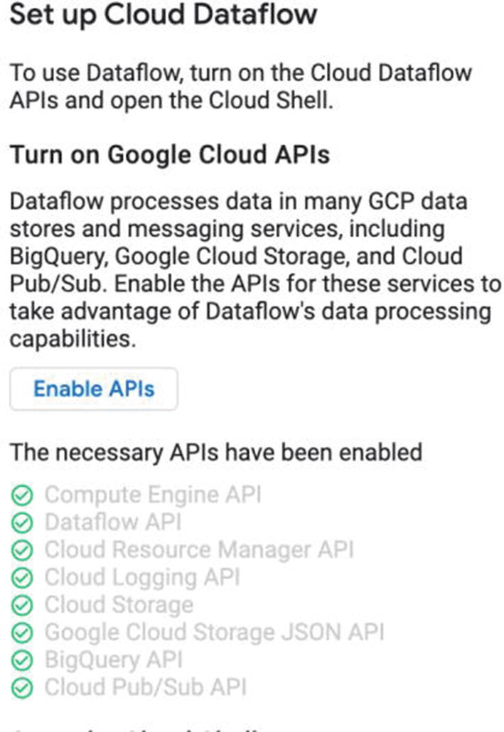
Figure 7-7.
You may have some or all of these turned on already, but clicking “Enable APIs” does the hard work for you and sets them all up.
The tutorial also recommends that you use the cloud shell to deploy a sample job. I concur with this: if you happen to have a Python 3.x environment on your local machine, you can do it there, but the cloud shell already has Python and pip (the Python package manager) installed—and is pre-authenticated! It’s also disposable, so make sure you familiarize yourself with the expiration rules (see Appendix A) before storing scripts on it that you don’t want to lose.
If you are more comfortable with Java, there is thankfully a host of documentation available. The official Apache Beam documentation is equally fluent in Java and Python, but leaves out Go. The Google documentation also has samples in Go. Historically, the Java SDK has been superior to Python; while the gap has closed, I only choose Python here to keep the book’s primary language choice consistent.
Tutorial Annotation
I’m also not going to replicate the tutorial steps here and reinvent the wheel (a little Python humor there), but I will annotate each step to provide context for the demo against what we’ve covered already. GCP tutorials are amazing and easy to run. In fact, they are sometimes so easy that you aren’t sure what you’ve just done or its significance. This is not a criticism! No one wants to spend hours wrestling with operating systems and package dependencies just to see “Hello World.” It does, however, provide a great opportunity to apply the theory.

pip3 install --quiet apache-beam[gcp]
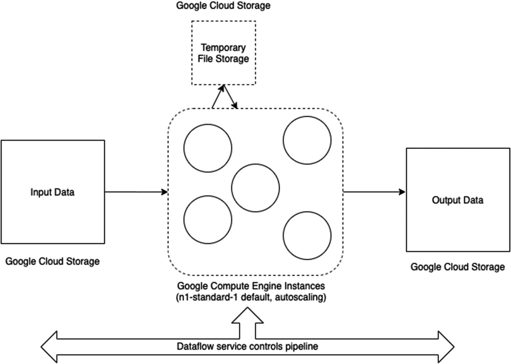
infrastructure for running Dataflow jobs in GCP
The missing piece to get going is that the GCP runner will need some place to store files that it can get to, both for input and output and also for temporary storage. Conveniently that location is Google Cloud Storage. You’ll need a location to store things no matter what runner you’re using. The tutorial has you create such a bucket—it uses the shell for this too, but you could also hop over to the Cloud Storage UI and make a bucket yourself.
Now that you have the pipeline, the sample files, and a place to put them, you can deploy the pipeline to the Cloud Dataflow service. To do that, you’re running python with the -m flag, which indicates you want to run a module as a script. That module is an Apache Beam sample that specifies that you want to run a job with a specific, unique name in GCP using the DataflowRunner , which is the name for Dataflow in Beam. You also specify the scratch location and a location for the output and the GCP project you want this all to take place in. And…that’s it. Once you run that command, you’ll start seeing INFO messages from Python appear in the shell telling you interesting things about the job’s current status. After some time, you’ll see that the job has finished and produced result files.
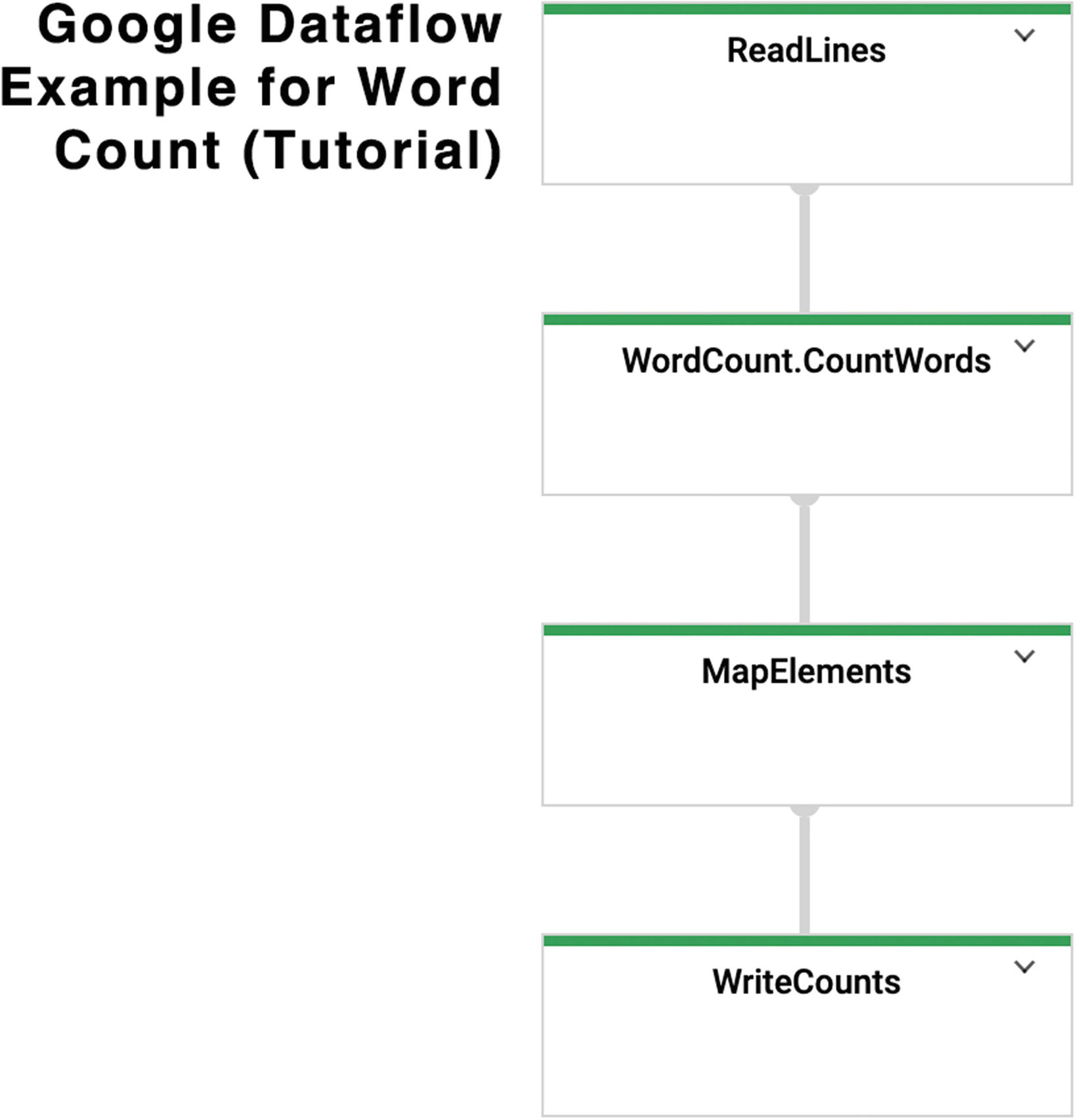
My favorite part about this whole tutorial is that it doesn’t actually tell you what you are doing. As it turns out, it takes the text of Shakespeare’s “King Lear” and counts the number of times each word appears. Before you go and look at the helpful UI representation of the pipeline, see if you can figure out which PTransforms it needed to do this.
Google Dataflow Runner
One really nice convenience about using Google Dataflow is that it gives you such a helpful graphical view into what is currently going on. I have a deep and abiding love for console logs, but being able to see what’s happening—and share with your coworkers—is very valuable.
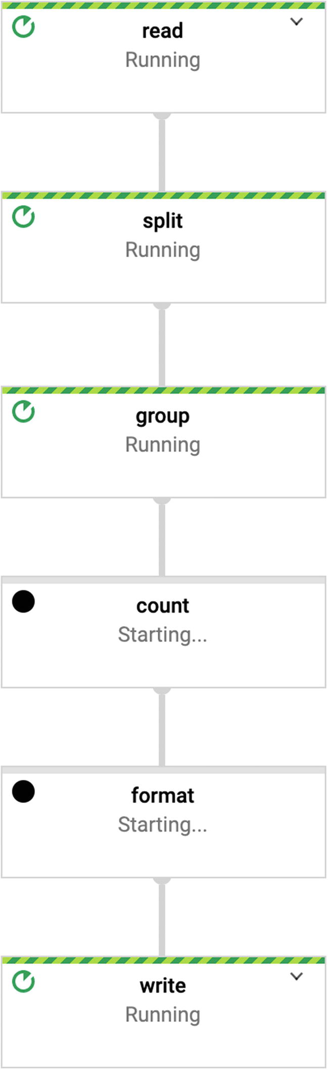
graph view of Dataflow
You can see the metrics for the full job, which is useful for troubleshooting steps that might be slow or jobs that are not effectively parallelizing. It can also help you make sure that the cost of your jobs remains reasonable.
Finally, you can view the logs for all of the workers that processed the job, which you can use to troubleshoot jobs that aren’t working the way you expect. Both these logs and the metrics are logged to Cloud Logging and Monitoring (formerly Stackdriver), which we’ll cover in depth in Chapter 12.
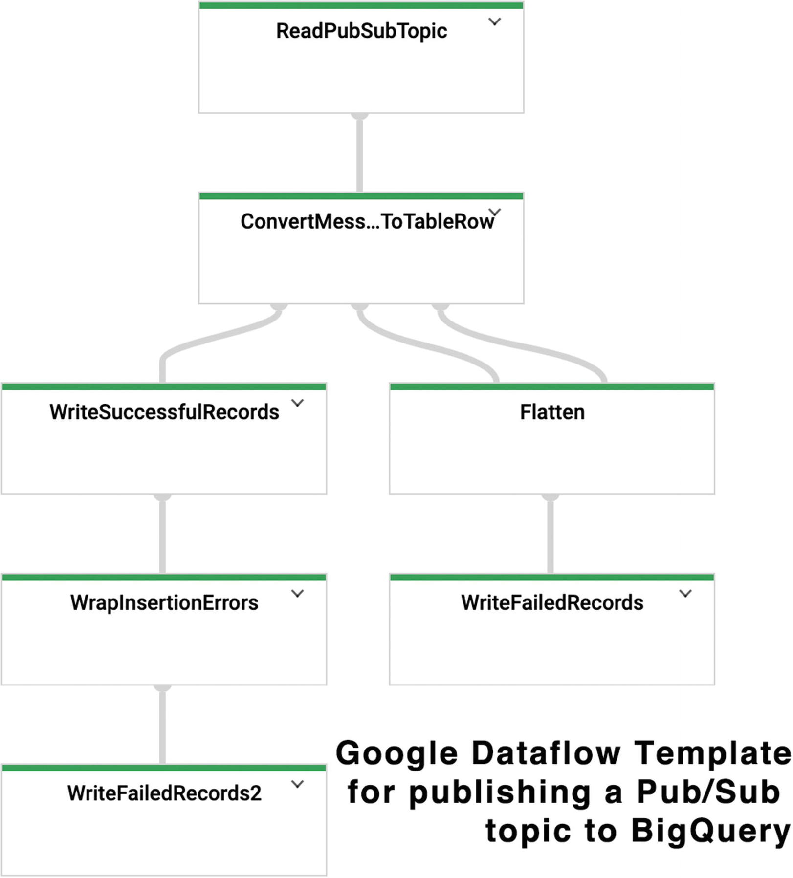
Dataflow Templates
For many tasks, there are predefined Dataflow templates you can use rather than building one yourself. Clicking “Create Dataflow Job from Template” in the top bar of the Dataflow console will open the page to do so.
Google Cloud Storage to BigQuery with data loss prevention: Uses Cloud DLP in the pipeline between GCS and BigQuery to automatically obfuscate sensitive data in uploaded files before loading it
Kafka to BigQuery: Takes a Kafka topic and Bootstrap Server list and pipes the streams on an ongoing basis into a BigQuery table
JDBC to BigQuery: Automates the exercise from Chapter 5 where we discussed hitting an arbitrary data source with a JDBC-compliant driver and loading the results into a BigQuery table
Most of the templates come with an associated tutorial you can use to replicate the underlying pipeline. These templates are all Java-based, as far as I could see, but you don’t need to get into the code to run the defaults.
Dataflow SQL
Now that you’ve seen the power of setting up a Dataflow, imagine doing it purely in SQL, using the same concepts we have used for querying and joining in BigQuery. Dataflow SQL became generally available in May 2020, and it’s already heralded a new world for constructing data processing pipelines. (Credit where credit is due, of course. Google Cloud Dataflow is only possible because of the joint development of Apache Beam SQL.)
Beam SQL sits on top of Beam Java to allow SQL queries to become PTransforms for the Java runner. When using Apache Beam Java directly, you can use both SQL PTransforms and regular PTransforms interchangeably. This also means that you might be able to upgrade some of your existing pipelines with SQL where appropriate.
Key Concept Extensions
Beam SQL uses two dialects of SQL. One, Calcite SQL is a variant of the Apache Calcite dialect. While it’s the default Beam SQL dialect, we won’t be using it here since our primary focus is BigQuery. The other dialect, ZetaSQL, is a language that was created at Google and open source in 2019. We’ll use it here since it is in fact the same SQL dialect used by BigQuery.
If you used BigQuery at its inception, you may recall that there was a second dialect of SQL there too, now called Legacy SQL. We don’t use BigQuery Legacy SQL anywhere in this book since it is no longer recommended by Google. I call this out to indicate that ZetaSQL may not be the predominant language extension even a few years after this book goes to print. This area of data processing is changing rapidly, and many people are contributing to repos to explore and standardize this. Hopefully this makes clear why I try to focus on the underlying concepts and their practical application to business. The concepts don’t change: Euler invented graph theory in the 18th century, and it’s just as applicable today. Edgar F. Codd codified relational algebra in 1970, but the underpinnings go back much further. Don’t sweat it—if you need to learn EtaSQL or ThetaSQL, so be it. That being said, Google has a decent track record at keeping their standards supported,1 and the goal of ZetaSQL—to unify the SQL dialect used across Google Cloud—is a good point in favor of its longevity.
The following are some additional terms you need to understand Beam SQL.
SqlTransform
The SqlTransform extends the PTransform class and defines transforms that are generated from SQL queries. (Beam allows you to initialize the runner with either Calcite SQL or ZetaSQL by default; as in the preceding text, we’ll use ZetaSQL.)
Row
A row is an object representing a SQL-specific element, namely, the row of a table. Rather than using the table nomenclature, the Java implementation appropriately uses the collection PCollection<Row> to represent a database table.
Dataflow SQL Extensions
In order for Dataflow SQL to have the expressiveness required to handle external data sources and processing pipelines, a few extensions to standard SQL are required. This is where the ZetaSQL dialect comes in. Its analyzer and parser have the extra keywords required to define SQL statements that can be converted into Apache Beam’s PTransforms.
Inputs and Outputs
Currently, Dataflow SQL can accept inputs from three GCP services: BigQuery itself, Cloud Storage, and Pub/Sub. It can supply outputs to two of those: BigQuery and Pub/Sub. You do accept a reduction in customization from working in Dataflow SQL. However, since Pub/Sub is so widely used as an asynchronous mechanism outside of data processing and Google Cloud Storage is an easy destination to integrate with file-based systems, you can shift the burden of data collation to outside of the pipeline itself. (In Chapter 11, we’ll talk about doing data transformation using Google Cloud Functions. You could just as easily have a Cloud Function pipe its results to a Pub/Sub queue, which would then attach to a Dataflow job.)
Formatting
Constructing pipelines in Dataflow SQL entails some specific formatting restrictions. At this time, messages arriving from Pub/Sub queues must be JSON-formatted. Avro support should be available by the time you read this. They must also be configured as a data source in BigQuery, and they must have schemas that are compatible with BigQuery. These restrictions make sense—even if you were writing your own pipeline in Java or Python, you have to match a BigQuery schema to insert data anyway.
Windowing
Recall that Dataflow is designed to work as easily with bounded data sources as with streaming (unbounded) sources. If you are using an unbounded data source like a Pub/Sub queue, you can’t simply use a key—the key may keep recurring in the incoming dataset, and you will never have a completely materialized “table” to work with. The solution to this is windowing. Windowing uses the timestamp of the incoming data as a key to logically divide the data into different durations. The elements in these data windows comprise the aggregation that is used as the input PCollection to the pipeline. This mechanism continues for the lifetime of the job.
There are two other methods of dividing unbounded datasets, known as watermarks and triggers. Neither is currently supported in Dataflow SQL. For more information, you can learn more about streaming pipelines at https://cloud.google.com/dataflow/docs/concepts/streaming-pipelines.
Types of Windows
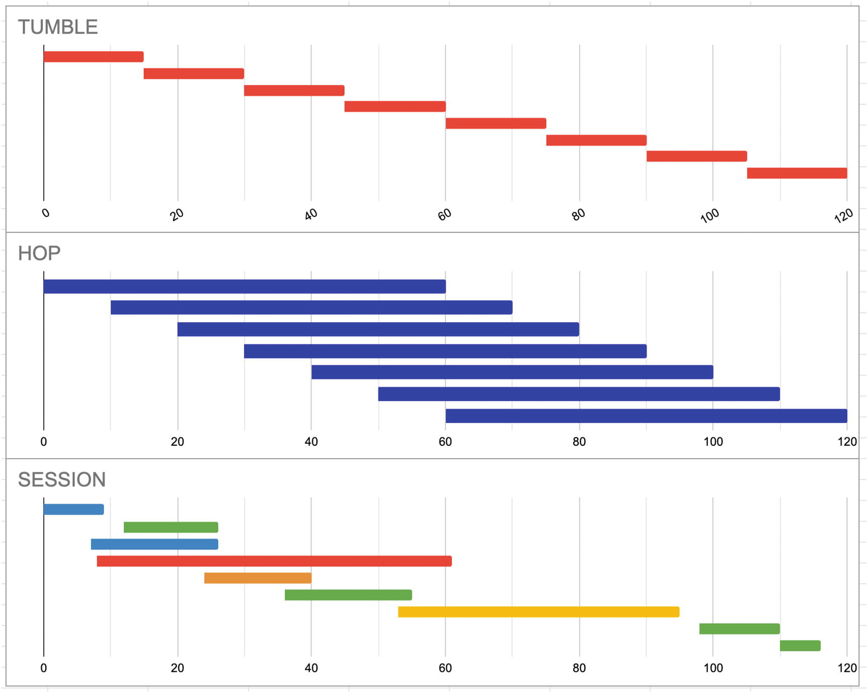
windowing types
Tumble
A tumble is a fixed interval that does not overlap with other windows. If you specify a tumble of 15 seconds, this means data will be aggregated every 15 seconds, in 15-second increments.
Pick an interval that gives you the best compromise between latency and cost. If users are only looking at the data on an hourly basis, there’s no need to run it with second-level frequency. On the other hand, if you’re receiving data constantly and need to immediately process and forward it, set a small interval.
Hop
Hop defines a fixed interval, but it may overlap with other windows. For example, you may want to see a minute worth of data, but you want it to roll a new minute window every ten seconds (i.e., 0:00–1:00, 0:10–1:10, 0:20–1:20, etc.).
This is useful for times when you want to be able to generate rolling averages over time. You may need a minute’s worth of data to do the processing, but you want to see an update every ten seconds.
Session
A session will collect data until a certain amount of time elapses with no data. Unlike tumble and hop, a session will also assign a new window to each data key.
The best use case for sessions is—unsurprisingly—user session data. If you are capturing user activity on a real-time basis, you want to continue to aggregate over that key (the session or user ID) until the user stops the activity. Then you can take the entire activity’s data and process it as one window. All you need to do is define the amount of time a key’s activity is idle before it is released.
Remember, if you are joining tables, you must ensure their windows are compatible. Data must be aggregated from all of the streaming data sources with the same frequency and timing.
Creating a Dataflow SQL Pipeline
And now, the fun part. Let’s see where you do this. The most interesting part of all of this is that you will literally not need to write a single line of code. You can make a SQL pipeline without knowing anything about PTransforms or DoFns or any such thing.
In fact, to create a Dataflow SQL pipeline, you don’t even need to go into the Dataflow console itself. The Dataflow mode is set up through the BigQuery UI. Once you create a job, you’ll be able to watch its deployment and progress through the Dataflow UI.
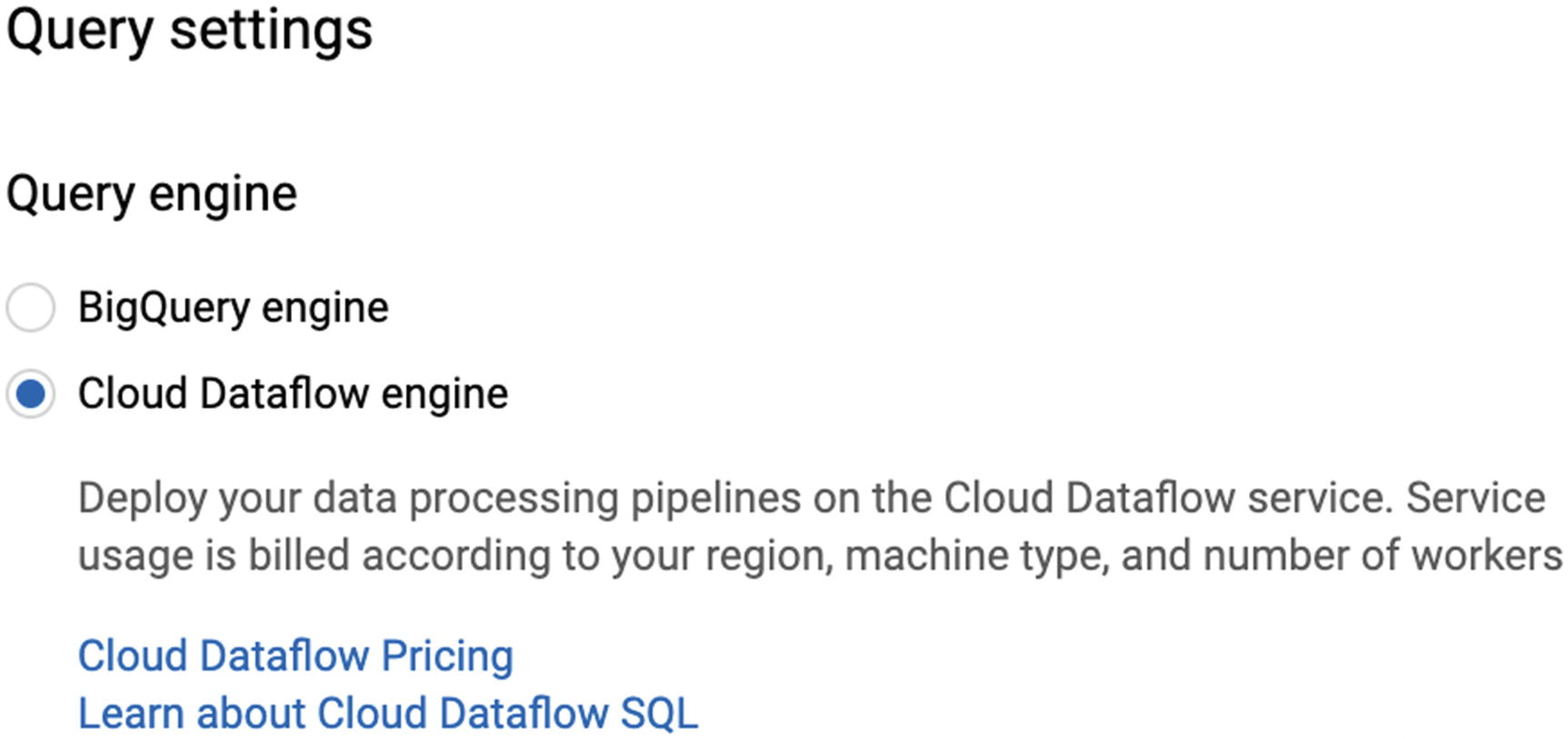
Figure 7-12.
Select Cloud Dataflow engine and click Save. Now, instead of running on BigQuery, you will see that the tag “Cloud Dataflow engine” has appeared and query execution has been replaced with “Create Cloud Dataflow job.”
In order to add sources from Dataflow, click “+ Add Data” next to Resources and click “Cloud Dataflow Sources.” This will bring up a window from which you can automatically search your project for valid Pub/Sub or Cloud Storage sources. (You can actually configure a Dataflow job from the Pub/Sub console as well with “Create Subscription.” This will allow you to choose a template from a list of supported Google Cloud operations.)
Once you select the source you want, a “Cloud Dataflow resources” section will appear in the Resources hierarchy with your topic below. The last thing to do is to configure the schema for incoming messages. Only JSON is supported right now, and the JSON must contain an “event_timestamp” field of type TIMESTAMP. (The UI actually lets you delete this required field. Don’t do that.)
Supply the schema in which you expect messages to arrive from the topic. This schema definition is the same as for BigQuery tables, so you can also “edit as text” and paste in the schema from one of your existing tables.
Now that that’s done, you’re free to use this streaming data source as if it were a regular table in BigQuery, plus the addition of a windowing aggregate if you want one. That’s it! No Java, no Python, and no PCollections or PTransforms, just (almost) plain old SQL.
This query, when converted to a Dataflow job, will collect the live sales from a Pub/Sub and then join to an existing BigQuery table to get the name and total sales of that item automatically. You can then pipe the result anywhere else you like.
Note the additional prefix of “bigquery.table.” required to reach the table from Dataflow. Even though you’re in the BigQuery UI, you’re using the Dataflow SQL engine, and the syntax is a little different. (None of the “tumble” stuff would work in BigQuery SQL either.)
Deploying Your Dataflow SQL Job
Now that you have written your query, it’s time to convert it into a Dataflow pipeline. This means GCP will be handling the underlying Java runner, creating a SqlTransform object from your query, generating the pipeline, and deploying it to the Cloud Dataflow runner. You don’t have to do any of this manually, but aren’t you glad you know how much work that would have been?
When you click “Create Cloud Dataflow job,” you will have to go through a bit more ceremony than your average five-line SQL query requires. Let’s walk through the options available to us, since we no longer have access to the underlying code in which to write them ourselves. (These parameters are available in Java/Python jobs as configurations too.)
Name and Region
Choose a descriptive name that is unique among your running jobs. This is the job name you’ll see in the Dataflow console, so pick something you’ll be able to recognize.
Dataflow pipelines run by default in the us-central1 region. You can modify the zone in which your underlying worker instances will run. You may need to control this for compliance reasons but otherwise can leave it alone.
Max Workers
This is the number of Google Compute Engines the pipeline will use. You can prioritize cost over time or leave allocation for other, higher-priority jobs by changing this number.
Worker Region/Zone
As mentioned earlier, you can actually specify that the Google Compute Engine VMs use a different region than the job is using. You can further specify the zone they will operate in within that region. Google recommends not setting the zone, as they can more efficiently optimize the job by choosing the zone themselves.
Service Account Email
The service account is the security principal used for the execution of the job. (It’s like a username for robots.) GCP will generally create a new service account when one is needed, but if you have one with permissions or security that you need, you can specify it directly.
Machine Type
Since Dataflow jobs are building and tearing down virtual machines on the fly, you can specify what kind of virtual machine you want to be used as a worker.
Network Configurations
With these configurations, you can assign the network and subnetwork you want the virtual machines assigned to. If you have protected resources in a certain network needed for the job to run, you will want the VMs to run in that network as well. You can also specify whether the virtual machines will have public or internal IPs. Note that some runners (like Python) actually need Internet access in order to reach their package repositories upon spin-up, so you might not want to touch this. If you want the machines to have both internal IPs and limited Internet access, you will have to perform all the NATing yourself—contact an experienced cloud engineer!
Destination
This section is how you specify where you would like the results of the job to go. As referenced earlier, the two options are Pub/Sub and BigQuery. Selecting either of these will open up the required options to select/create either a Pub/Sub topic or a BigQuery dataset table.
Note also that you can check the box marked “Additional Output” and specify a second output for the job. This gives you the ability to store your results in a BigQuery table and also to send the results to a Pub/Sub, which you could then connect to another pipeline or a Cloud Function or anything else!
Creating the Job
After you click “Create,” GCP will get to work. It can take a couple minutes for it to prepare everything, but you’ll be able to see it in the BigQuery UI, the Dataflow UI, and the Pub/Sub UI (if applicable). Dataflow will follow the same steps that you did when you deployed the Python pipeline. Once it has done this, the workflow graph will appear in the UI, and you will be able to track metrics and CPU utilization. This job will run until you manually stop it.
And there you have it! You now have everything you need to do real-time processing on massive, unbounded datasets without needing to do any manual administration whatsoever. Now go out there and get the rest of your organization’s data into BigQuery.
One final note: This is where things can start getting expensive. Running a continuous streaming job from Pub/Sub to BigQuery involves having Google Compute Engine VMs running constantly, plus the cost of BigQuery, Pub/Sub, and Dataflow themselves. Batch jobs can be relatively cheap, but streaming will incur charge for as long as you have the pipeline up and running. Don’t let this deter you, but if you are running intensive processing on large amounts of data, keep an eye on your bill.
Summary
Google Dataflow is a powerful data processing technology built on Apache Beam, an open source project originally incubated at Google. Dataflow allows you to write massively parallelized load and transformation jobs easily and deploy them scalably to Google Cloud. Although originally Dataflow and Beam supported only procedural languages like Java, Python, and Go, they recently introduced Dataflow SQL, which allows you to write your transformations in pure SQL. Regardless of the method you choose, building your own Dataflow jobs can allow you to quickly and reliably process huge amounts of data into BigQuery.