Chapter 8. Techniques of Estimation
8.1. Objectives*
After completing this chapter, you should
Estimation by Rounding (Section 8.2)
understand the reason for estimation
be able to estimate the result of an addition, multiplication, subtraction, or division using the rounding technique
Estimation by Clustering (Section 8.3)
understand the concept of clustering
be able to estimate the result of adding more than two numbers when clustering occurs using the clustering technique
Mental Arithmetic—Using the Distributive Property (Section 8.4)
understand the distributive property
be able to obtain the exact result of a multiplication using the distributive property
Estimation by Rounding Fractions (Section 8.5)
be able to estimate the sum of two or more fractions using the technique of rounding fractions
8.2. Estimation by Rounding*
Section Overview
Estimation By Rounding
When beginning a computation, it is valuable to have an idea of what value to expect for the result. When a computation is completed, it is valuable to know if the result is reasonable.
In the rounding process, it is important to note two facts:
The rounding that is done in estimation does not always follow the rules of rounding discussed in Section 1.4 (Rounding Whole Numbers). Since estimation is concerned with the expected value of a computation, rounding is done using convenience as the guide rather than using hard-and-fast rounding rules. For example, if we wish to estimate the result of the division 80 ÷ 26, we might round 26 to 20 rather than to 30 since 80 is more conveniently divided by 20 than by 30.
Since rounding may occur out of convenience, and different people have different ideas of what may be convenient, results of an estimation done by rounding may vary. For a particular computation, different people may get different estimated results. Results may vary.
Estimation is the process of determining an expected value of a computation.
Common words used in estimation are about, near, and between.
Estimation by Rounding
The rounding technique estimates the result of a computation by rounding the numbers involved in the computation to one or two nonzero digits.
Sample Set A
Example 8.1.
Estimate the sum: 2,357 + 6,106.
Notice that 2,357 is near  and that 6,106 is near
The sum can be estimated by 2,400 + 6,100 = 8,500. (It is quick and easy to add 24 and 61.)
Thus, 2,357 + 6,106 is about 8,400. In fact, 2,357 + 6,106 = 8,463.
Practice Set A
Sample Set B
Example 8.2.
Estimate the difference: 5,203 – 3,015.
Notice that 5,203 is near  and that 3,015 is near
The difference can be estimated by 5,200 – 3,000 = 2,200.
Thus, 5,203 – 3,015 is about 2,200. In fact, 5,203 – 3,015 = 2,188.
We could make a less accurate estimation by observing that 5,203 is near 5,000. The number 5,000 has only one nonzero digit rather than two (as does 5,200). This fact makes the estimation quicker (but a little less accurate). We then estimate the difference by 5,000 – 3,000 = 2,000, and conclude that 5,203 – 3,015 is about 2,000. This is why we say "answers may vary."
Practice Set B
Sample Set C
Example 8.3.
Estimate the product: 73 ⋅ 46.
Notice that 73 is near  and that 46 is near
The product can be estimated by 70 ⋅ 50 = 3,500. (Recall that to multiply numbers ending in zeros, we multiply the nonzero digits and affix to this product the total number of ending zeros in the factors. See Section 2.2 for a review of this technique.)
Thus, 73 ⋅ 46 is about 3,500. In fact, 73 ⋅ 46 = 3,358.
Example 8.4.
Estimate the product: 87 ⋅ 4,316.
Notice that 87 is close to  and that 4,316 is close to
The product can be estimated by 90 ⋅ 4,000 = 360,000.
Thus, 87 ⋅ 4,316 is about 360,000. In fact, 87 ⋅ 4,316 = 375,492.
Practice Set C
Sample Set D
Example 8.5.
Estimate the quotient: 153 ÷ 17.
Notice that 153 is close to  and that 17 is close to
The quotient can be estimated by 150 ÷ 15 = 10.
Thus, 153 ÷ 17 is about 10. In fact, 153 ÷ 17 = 9.
Example 8.6.
Estimate the quotient: 742,000 ÷ 2,400.
Notice that 742,000 is close to  , and that 2,400 is close to
The quotient can be estimated by 700,000 ÷ 2,000 = 350.
Thus,
742,000 ÷ 2,400 is about 350. In fact,
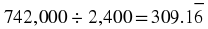 .
.
Practice Set D
Sample Set E
Example 8.7.
Estimate the sum: 53.82 + 41.6.
Notice that 53.82 is close to  and that 41.6 is close to
The sum can be estimated by 54 + 42 = 96.
Thus, 53.82 + 41.6 is about 96. In fact, 53.82 + 41.6 = 95.42.
Practice Set E
Sample Set F
Example 8.8.
Estimate the product: (31.28)(14.2).
Notice that 31.28 is close to  and that 14.2 is close to
The product can be estimated by 30 ⋅ 15 = 450. ( 3 ⋅ 15 = 45, then affix one zero.)
Thus, (31.28)(14.2) is about 450. In fact, (31.28)(14.2) = 444.176.
Example 8.9.
Estimate 21% of 5.42.
Notice that
21% = .21 as a decimal, and that .21 is close to 
Notice also that 5.42 is close to 
Then, 21% of 5.42 can be estimated by (.2)(5) = 1.
Thus, 21% of 5.42 is about 1. In fact, 21% of 5.42 is 1.1382.
Practice Set F
Exercises
Estimate each calculation using the method of rounding. After you have made an estimate, find the exact value and compare this to the estimated result to see if your estimated value is reasonable. Results may vary.
Exercise 8.2.18.
3,481 + 4,216
Exercise 8.2.20.
611 + 806
Exercise 8.2.22.
6,476 + 7,814
Exercise 8.2.24.
8,427 − 5,342
Exercise 8.2.26.
26,486 − 18,931
Exercise 8.2.28.
67⋅42
Exercise 8.2.30.
426⋅741
Exercise 8.2.32.
22,481⋅51,076
Exercise 8.2.34.
884÷33
Exercise 8.2.36.
2,189÷42
Exercise 8.2.38.
2,688÷48
Exercise 8.2.40.
43.016 + 47.58
Exercise 8.2.42.
115.0012 − 25.018
Exercise 8.2.44.
592.131 + 211.6
Exercise 8.2.46.
(87.013)(21.07)
Exercise 8.2.48.
(6.032)(14.091)
Exercise 8.2.50.
(5,137.118)(263.56)
Exercise 8.2.52.
(83.04)(1.03)
Exercise 8.2.54.
(14.016)(.016)
Exercise 8.2.56.
107% of 12.6
Exercise 8.2.58.
74% of 21.93
Exercise 8.2.60.
4% of .863
Exercises for Review


Exercise 8.2.65. (Go to Solution)
(Section 7.4) A woman 5 foot tall casts an 8-foot shadow at a particular time of the day. How tall is a tree that casts a 96-foot shadow at the same time of the day?
Solutions to Exercises
Solution to Exercise 8.2.1. (Return to Exercise)
4,216 + 3,942 : 4,200 + 3,900 . About 8,100. In fact, 8,158.
Solution to Exercise 8.2.2. (Return to Exercise)
812 + 514 : 800 + 500 . About 1,300. In fact, 1,326.
Solution to Exercise 8.2.3. (Return to Exercise)
43,892 + 92,106 : 44,000 + 92,000 . About 136,000. In fact, 135,998.
Solution to Exercise 8.2.5. (Return to Exercise)
7,842 – 5,209 : 7,800 – 5,200 . About 2,600. In fact, 2,633.
Solution to Exercise 8.2.6. (Return to Exercise)
73,812 – 28,492 : 74,000 – 28,000 . About 46,000. In fact, 45,320.
Solution to Exercise 8.2.11. (Return to Exercise)
4,079 ÷ 381 : 4,000 ÷ 400 . About 10. In fact, 10.70603675...
Solution to Exercise 8.2.12. (Return to Exercise)
609,000 ÷ 16,000 : 600,000 ÷ 15,000 . About 40. In fact, 38.0625.
Solution to Exercise 8.2.13. (Return to Exercise)
61.02 + 26.8 : 61 + 27 . About 88. In fact, 87.82.
Solution to Exercise 8.2.14. (Return to Exercise)
109.12 + 137.88 : 110 + 138 . About 248. In fact, 247. We could have estimated 137.88 with 140. Then 110 + 140 is an easy mental addition. We would conclude then that 109.12 + 137.88 is about 250.
Solution to Exercise 8.2.15. (Return to Exercise)
( 47.8 ) ( 21.1 ) : ( 50 ) ( 20 ) . About 1,000. In fact, 1,008.58.
Solution to Exercise 8.2.16. (Return to Exercise)
32% of 14.88 : ( .3 ) ( 15 ). About 4.5. In fact, 4.7616.

8.3. Estimation by Clustering*
Section Overview
Estimation by Clustering
When more than two numbers are to be added, the sum may be estimated using the clustering technique. The rounding technique could also be used, but if several of the numbers are seen to cluster (are seen to be close to) one particular number, the clustering technique provides a quicker estimate. Consider a sum such as
32 + 68 + 29 + 73
Notice two things:
There are more than two numbers to be added.
Clustering occurs.
Both 68 and 73 cluster around 70, so 68 + 73 is close to 80 + 70 = 2(70) = 140.
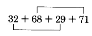
Both 32 and 29 cluster around 30, so 32 + 29 is close to 30 + 30 = 2(30) = 60.
The sum may be estimated by
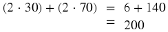
In fact, 32 + 68 + 29 + 73 = 202.
Sample Set A
Estimate each sum. Results may vary.
Example 8.10.
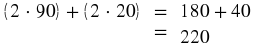
27 + 48 + 31 + 52.
27 and 31 cluster near 30. Their sum is about 2 ⋅ 30 = 60.
48 and 52 cluster near 50. Their sum is about 2 ⋅ 50 = 100.
Thus,
27 + 48 + 31 + 52 is about
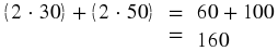
In fact, 27 + 48 + 31 + 52 = 158.
Example 8.11.
88 + 21 + 19 + 91.
88 and 91 cluster near 90. Their sum is about 2 ⋅ 90 = 180.
21 and 19 cluster near 20. Their sum is about 2 ⋅ 20 = 40.
Thus,
88 + 21 + 19 + 91 is about
In fact, 88 + 21 + 19 + 91 = 219.
Example 8.12.
17 + 21 + 48 + 18.
17, 21, and 18 cluster near 20. Their sum is about 3 ⋅ 20 = 60.
48 is about 50.
Thus,
17 + 21 + 48 + 18 is about
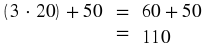
In fact, 17 + 21 + 48 + 18 = 104.
Example 8.13.
61 + 48 + 49 + 57 + 52.
61 and 57 cluster near 60. Their sum is about 2 ⋅ 60 = 120.
48, 49, and 52 cluster near 50. Their sum is about 3⋅ 50 = 150.
Thus,
61 + 48 + 49 + 57 + 52 is about
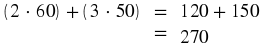
In fact, 61 + 48 + 49 + 57 + 52 = 267.
Example 8.14.
706 + 321 + 293 + 684.
706 and 684 cluster near 700. Their sum is about 2 ⋅ 700 = 1,400.
321 and 293 cluster near 300. Their sum is about 2 ⋅ 300 = 600.
Thus,
706 + 321 + 293 + 684 is about
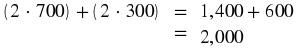
In fact, 706 + 321 + 293 + 684 = 2,004.
Practice Set A
Use the clustering method to estimate each sum.
Exercises
Use the clustering method to estimate each sum. Results may vary.
Exercise 8.3.6.
42 + 19 + 39 + 23
Exercise 8.3.8.
76 + 29 + 33 + 82
Exercise 8.3.10.
41 + 28 + 42 + 37
Exercise 8.3.12.
73 + 72 + 27 + 71
Exercise 8.3.14.
31 + 77 + 31 + 27
Exercise 8.3.16.
94 + 18 + 23 + 91 + 19
Exercise 8.3.18.
42 + 121 + 119 + 124 + 41
Exercise 8.3.20.
108 + 61 + 63 + 96 + 57 + 99
Exercise 8.3.22.
981 + 1208 + 1214 + 1006
Exercise 8.3.24.
94 + 68 + 66 + 101 + 106 + 71 + 110
Exercises for Review

Exercise 8.3.29. (Go to Solution)
(Section 8.2) Estimate the sum using the method of rounding: 4,882 + 2,704.
Solutions to Exercises

8.4. Mental Arithmetic-Using the Distributive Property*
Section Overview
The Distributive Property
Estimation Using the Distributive Property
The Distributive Property
The distributive property is a characteristic of numbers that involves both addition and multiplication. It is used often in algebra, and we can use it now to obtain exact results for a multiplication.
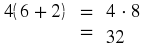
Suppose we wish to compute 3(2 + 5). We can proceed in either of two ways, one way which is known to us already (the order of operations), and a new way (the distributive property).
-
Compute
3(2 + 5) using the order of operations.
3 ( 2 + 5 )
Operate inside the parentheses first: 2 + 5 = 7.
3 ( 2 + 5 ) = 3 ⋅ 7
Now multiply 3 and 7.
3 ( 2 + 5 ) = 3 ⋅ 7 = 21
Thus, 3(2 + 5) = 21.
-
Compute
3(2 + 5) using the distributive property.
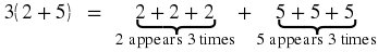
We know that multiplication describes repeated addition. Thus,
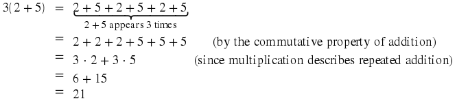
Thus, 3(2 + 5) = 21.
Let's look again at this use of the distributive property.

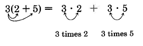
The 3 has been distributed to the 2 and 5.
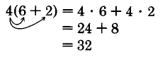
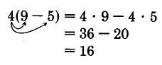
This is the distributive property. We distribute the factor to each addend in the parentheses. The distributive property works for both sums and differences.
Sample Set A
Example 8.15.
Using the order of operations, we get
Example 8.16.
Using the order of operations, we get

Example 8.17.
Example 8.18.
Practice Set A
Use the distributive property to compute each value.
Estimation Using the Distributive Property
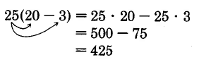
We can use the distributive property to obtain exact results for products such as 25 ⋅ 23. The distributive property works best for products when one of the factors ends in 0 or 5. We shall restrict our attention to only such products.
Sample Set B
Use the distributive property to compute each value.
Example 8.19.
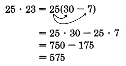
25 ⋅ 23
Notice that 23 = 20 + 3. We now write
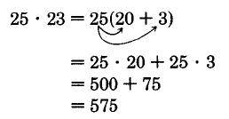
Thus, 25 ⋅ 23 = 575
We could have proceeded by writing 23 as 30 – 7.
Example 8.20.
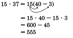
15 ⋅ 37
Notice that 37 = 30 + 7. We now write
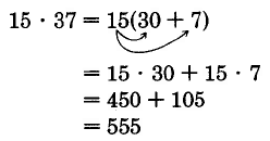
Thus, 15 ⋅ 37 = 555
We could have proceeded by writing 37 as 40 – 3.
Example 8.21.
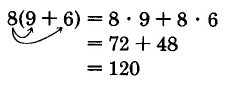
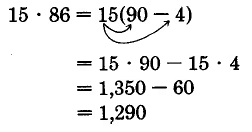
15 ⋅ 86
Notice that 86 = 80 + 6. We now write
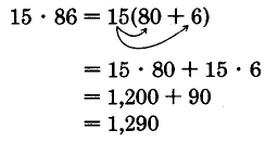
We could have proceeded by writing 86 as 90 – 4.
Practice Set B
Use the distributive property to compute each value.
Exercises
Use the distributive property to compute each product.
Exercise 8.4.13.
15⋅14
Exercise 8.4.15.
25⋅16
Exercise 8.4.17.
35⋅12
Exercise 8.4.19.
45⋅38
Exercise 8.4.21.
25⋅96
Exercise 8.4.23.
85⋅34
Exercise 8.4.25.
55⋅51
Exercise 8.4.27.
25⋅208
Exercise 8.4.29.
85⋅110
Exercise 8.4.31.
65⋅40
Exercise 8.4.33.
30⋅47
Exercise 8.4.35.
90⋅78
Exercises for Review


Solutions to Exercises
Solution to Exercise 8.4.24. (Return to Exercise)
65(20 + 6) = 1,300 + 390 = 1,690 or 65(30 − 4) = 1,950 − 260 = 1,690

8.5. Estimation by Rounding Fractions*
Section Overview
Estimation by Rounding Fractions
Estimation by rounding fractions is a useful technique for estimating the result of a computation involving fractions. Fractions are commonly rounded to
 ,
,
 ,
,
 , 0, and 1. Remember that rounding may cause estimates to vary.
Sample Set A
Make each estimate remembering that results may vary.
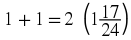
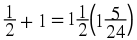
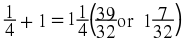
Example 8.22.
Estimate
 .
.
Notice that
 is about
 , and that
 is about
 .
.
Thus,
 is about
 . In fact,
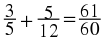 , a little more than 1.
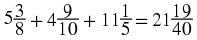
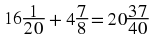
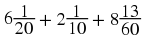
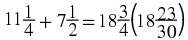
Example 8.23.
Estimate
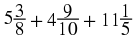 .
.
Adding the whole number parts, we get 20. Notice that
 is close to
 ,
,
 is close to 1, and
 is close to
 . Then
 is close to
 .
.
Thus,
 is close to
 .
.
In fact,
 , a little less than
 .
.
Practice Set A
Use the method of rounding fractions to estimate the result of each computation. Results may vary.


Exercises
Estimate each sum or difference using the method of rounding. After you have made an estimate, find the exact value of the sum or difference and compare this result to the estimated value. Result may vary.

Exercise 8.5.6.


Exercise 8.5.8.


Exercise 8.5.10.


Exercise 8.5.12.


Exercise 8.5.14.


Exercise 8.5.16.


Exercise 8.5.18.


Exercise 8.5.20.
Exercise 8.5.22.


Exercise 8.5.24.

Exercises for Review
Exercise 8.5.25. (Go to Solution)
(Section 2.6) The fact that (a first number ⋅ a second number) ⋅ a third number = a first number ⋅ (a second number ⋅ a third number ) is an example of which property of multiplication?


Exercise 8.5.29. (Go to Solution)
(Section 8.4) Use the distributive property to compute the product: 25 ⋅ 37.
Solutions to Exercises


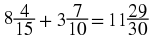
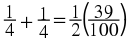
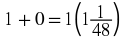
Solution to Exercise 8.5.4. (Return to Exercise)
Results may vary.
(16 + 0) + (4 + 1) = 16 + 5 = 21. In fact,


8.6. Summary of Key Concepts*
Summary of Key Concepts
Estimation is the process of determining an expected value of a computation.
The rounding technique estimates the result of a computation by rounding the numbers involved in the computation to one or two nonzero digits. For example, 512 + 896 can be estimated by 500 + 900 = 1,400.
When several numbers are close to one particular number, they are said to cluster near that particular number.
The clustering technique of estimation can be used when
there are more than two numbers to be added, and
clustering occurs.
For example, 31 + 62 + 28 + 59 can be estimated by ( 2 ⋅ 30 ) + ( 2 ⋅ 60 ) = 60 + 120 = 180
The distributive property is a characteristic of numbers that involves both addition and multiplication. For example, 3(4 + 6) = 3 ⋅ 4 + 3 ⋅ 6 = 12 + 18 = 30
The distributive property can be used to obtain exact results for a multiplication. For example, 15 ⋅ 23 = 15 ⋅ ( 20 + 3 ) = 15 ⋅ 20 + 15 ⋅ 3 = 300 + 45 = 345
Estimation by rounding fractions commonly rounds fractions to
 ,
,
 ,
,
 , 0, and 1. For example,
 can be estimated by

8.7. Exercise Supplement*
Exercise Supplement
Estimation by Rounding (Section 8.2)
For problems 1-70, estimate each value using the method of rounding. After you have made an estimate, find the exact value. Compare the exact and estimated values. Results may vary.
Exercise 8.7.2.
419 + 582
Exercise 8.7.4.
926 + 1,105
Exercise 8.7.6.
5,026 + 2,814
Exercise 8.7.8.
1,186 + 4,228
Exercise 8.7.10.
8,305 + 484
Exercise 8.7.12.
5,293 + 8,007
Exercise 8.7.14.
92,512 + 26,071
Exercise 8.7.16.
42,612 + 4,861
Exercise 8.7.18.
487,235 + 494
Exercise 8.7.20.
3,704 + 4,704
Exercise 8.7.22.
38⋅81
Exercise 8.7.24.
52⋅21
Exercise 8.7.26.
412⋅807
Exercise 8.7.28.
62⋅596
Exercise 8.7.30.
92⋅336
Exercise 8.7.32.
8⋅2,106
Exercise 8.7.34.
374⋅816
Exercise 8.7.36.
126⋅2,834
Exercise 8.7.38.
5,794⋅837
Exercise 8.7.40.
7,471⋅5,782
Exercise 8.7.42.
309÷16
Exercise 8.7.44.
527÷17
Exercise 8.7.46.
1,728÷36
Exercise 8.7.48.
2,562÷61
Exercise 8.7.50.
3,618÷18
Exercise 8.7.52.
7,476÷356
Exercise 8.7.54.
43,776÷608
Exercise 8.7.56.
51,492÷514
Exercise 8.7.58.
33,712÷112
Exercise 8.7.60.
176,978÷214
Exercise 8.7.62.
73.73 + 72.9
Exercise 8.7.64.
87.865 + 46.772
Exercise 8.7.66.
(48.3)(29.6)
Exercise 8.7.68.
(107.02)(48.7)
Exercise 8.7.70.
(1.07)(13.89)
Estimation by Clustering (Section 8.3)
For problems 71-90, estimate each value using the method of clustering. After you have made an estimate, find the exact value. Compare the exact and estimated values. Results may vary.
Exercise 8.7.72.
19 + 73 + 23 + 71
Exercise 8.7.74.
18 + 73 + 69 + 19
Exercise 8.7.76.
67 + 71 + 84 + 81
Exercise 8.7.78.
34 + 56 + 36 + 55
Exercise 8.7.80.
93 + 108 + 96 + 111
Exercise 8.7.82.
32 + 27 + 48 + 51 + 72 + 69
Exercise 8.7.84.
81 + 41 + 92 + 38 + 88 + 80
Exercise 8.7.86.
44 + 38 + 87
Exercise 8.7.88.
31 + 28 + 49 + 29
Exercise 8.7.90.
57 + 62 + 18 + 23 + 61 + 21
Mental Arithmetic- Using the Distributive Property (Section 8.4)
For problems 91-110, compute each product using the distributive property.
Exercise 8.7.92.
15⋅42
Exercise 8.7.94.
35⋅28
Exercise 8.7.96.
95⋅11
Exercise 8.7.98.
60⋅18
Exercise 8.7.100.
65⋅31
Exercise 8.7.102.
38⋅25
Exercise 8.7.104.
19⋅85
Exercise 8.7.106.
81⋅40
Exercise 8.7.108.
35⋅202
Exercise 8.7.110.
85⋅97
Estimation by Rounding Fractions (Section 8.5)
For problems 111-125, estimate each sum using the method of rounding fractions. After you have made an estimate, find the exact value. Compare the exact and estimated values. Results may vary.

Exercise 8.7.112.


Exercise 8.7.114.


Exercise 8.7.116.


Exercise 8.7.118.


Exercise 8.7.120.

Exercise 8.7.122.
Exercise 8.7.124.

Solutions to Exercises


8.8. Proficiency Exam*
Proficiency Exam
For problems 1 - 16, estimate each value. After you have made an estimate, find the exact value. Results may vary.
For problems 17-21, use the distributive property to obtain the exact result.
For problems 22-25, estimate each value. After you have made an estimate, find the exact value. Results may vary.