CHAPTER 2: Data Design and Implementation
© Repina Valeriya/Shutterstock
In Chapter 1, we looked at an overview of the design process and reviewed the software engineering principles that, if followed, lead to quality software. The role of testing at all phases of the software life cycle was stressed.
In this chapter, we lay out the logical framework from which we examine data structures. We look at data structures from three points of view: how they are specified, how they are implemented, and how they can be used. In addition, the object-oriented view of data objects is presented. Finally, we examine C++ constructs that can be used to ensure the data structures we construct are correct.
2.1 Different Views of Data
What Do We Mean by Data?
When we talk about the function of a program, we use words such as “add,” “read,” “multiply,” “write,” “do,” and so on. The function of a program describes what it does in terms of the verbs in the programming language.
The data are the nouns of the programming world: the objects that are manipulated, the information that is processed by a computer program. In a sense, this information is just a collection of bits that can be turned on or off. The computer itself needs to have data in this form. Humans, however, tend to think of information in terms of somewhat larger units such as numbers and lists, so we want at least the human-readable portions of our programs to refer to data in a way that makes sense to us. To separate the computer’s view of data from our own view, we use data abstraction to create other views. Whether we use functional decomposition to produce a hierarchy of tasks or object-oriented design to produce a hierarchy of cooperating objects, data abstraction is essential.
Data Abstraction
Many people feel more comfortable with things that they perceive as real than with things that they think of as abstract. As a consequence, “data abstraction” may seem more forbidding than a more concrete entity such as an “integer.” But let’s take a closer look at that very concrete—and very abstract—integer you’ve been using since you wrote your earliest programs.
Just what is an integer? Integers are physically represented in different ways on different computers. In the memory of one machine, an integer may be represented in two’s complement notation by 32 binary digits. In another machine it may be 64 binary digits, while in a third it may use only 16. Although you may not know what these terms mean, that lack of knowledge hasn’t stopped you from using integers. (You learn about these terms in an assembly language course, so we do not explain them here.)
The way that integers are physically represented determines how the computer manipulates them. As a C++ programmer, you rarely get involved at this level; instead, you simply use integers. All you need to know is how to declare an int type variable and what operations are allowed on integers: assignment, addition, subtraction, multiplication, division, and modulo arithmetic.
Consider the statement
distance = rate * time;
It’s easy to understand the concept behind this statement. The concept of multiplication doesn’t depend on whether the operands are, say, integers or real numbers, despite the fact that integer multiplication and floating-point multiplication may be implemented in very different ways on the same computer. Computers would not be so popular if every time we wanted to multiply two numbers we had to get down to the machine-representation level. But that isn’t necessary: C++ has surrounded the int data type with a nice, neat package and has given you just the information you need to create and manipulate data of this type.
Another word for “surround” is “encapsulate.” Think of the capsules surrounding the medicine you get from the pharmacist when you’re sick. You don’t have to know anything about the chemical composition of the medicine inside to recognize the big blue-and-white capsule as your antibiotic or the little yellow capsule as your decongestant. Data encapsulation means that the physical representation of a program’s data is surrounded. The user of the data doesn’t see the implementation, but deals with the data only in terms of its logical picture—its abstraction.
If the data are encapsulated, how can the user get to them? Operations must be provided to allow the user to create, access, and change data. Let’s look at the operations C++ provides for the encapsulated data type int. First, you can create (“construct”) variables of type int using declarations in your program. Then you can assign values to these integer variables by using the assignment operator or by reading values into them and perform arithmetic operations using +, -, *, /, and %. Figure 2.1 shows how C++ has encapsulated the type int in a tidy package.
The point of this discussion is that you have been dealing with a logical data abstraction of “integer” since the very beginning. The advantages of doing so are clear: You can think of the data and the operations in a logical sense and can consider their use without having to worry about implementation details. The lower levels are still there—they’re just hidden from you.
Remember that the goal in design is to reduce complexity through abstraction. We can extend this goal further: to protect our data abstraction through encapsulation. We refer to the set of all possible values (the domain) of an encapsulated data “object,” plus the specifications of the operations that are provided to create and manipulate the data, as an abstract data type (ADT for short).

Figure 2.1 A black box representing an integer
Data Structures
A single integer can be very useful if we need a counter, a sum, or an index in a program, but generally we must also deal with data that have lots of parts, such as a list. We describe the logical properties of such a collection of data as an ADT; we call the concrete implementation of the data a data structure. When a program’s information is made up of component parts, we must consider an appropriate data structure.
Data structures have a few features worth noting. First, they can be “decomposed” into their component elements. Second, the arrangement of the elements is a feature of the structure that affects how each element is accessed. Third, both the arrangement of the elements and the way they are accessed can be encapsulated.
Let’s look at a real-life example: a library. A library can be decomposed into its component elements—books. The collection of individual books can be arranged in a number of ways, as shown in Figure 2.2. Obviously, the way the books are physically arranged on the shelves determines how one would go about looking for a specific volume. The particular library with which we’re concerned doesn’t let its patrons get their own books, however; if you want a book, you must give your request to the librarian, who retrieves the book for you.

Figure 2.2 A collection of books ordered in different ways
The library “data structure” is composed of elements (books) in a particular physical arrangement; for instance, it might be ordered on the basis of the Dewey decimal system. Accessing a particular book requires knowledge of the arrangement of the books. The library user doesn’t have to know about the structure, however, because it has been encapsulated: Users access books only through the librarian. The physical structure and the abstract picture of the books in the library are not the same. The card catalog provides logical views of the library—ordered by subject, author, or title—that differ from its physical arrangement.
We use the same approach to data structures in our programs. A data structure is defined by (1) the logical arrangement of data elements, combined with (2) the set of operations we need to access the elements.
Notice the difference between an ADT and a data structure. The former is a high-level description: the logical picture of the data and the operations that manipulate them. The latter is concrete: a collection of data elements and the operations that store and retrieve individual elements. An ADT is implementation independent, whereas a data structure is implementation dependent. A data structure is how we implement the data in an ADT whose values have component parts. The operations on an ADT are translated into algorithms on the data structure.
Another view of data focuses on how they are used in a program to solve a particular problem—that is, their application. If we were writing a program to keep track of student grades, we would need a list of students and a way to record the grades for each student. We might take a by-hand grade book and model it in our program. The operations on the grade book might include adding a name, adding a grade, averaging a student’s grades, and so on. Once we have written a specification for our grade book data type, we must choose an appropriate data structure to implement it and design the algorithms to implement the operations on the structure.
In modeling data in a program, we wear many hats. That is, we must determine the logical picture of the data, choose the representation of the data, and develop the operations that encapsulate this arrangement. During this process, we consider data from three different perspectives, or levels:
Application (or user) level: A way of modeling real-life data in a specific context; also called the problem domain
Logical (or abstract) level: An abstract view of the data values (the domain) and the set of operations to manipulate them
Implementation level: A specific representation of the structure to hold the data items, and the coding of the operations in a programming language (if the operations are not already provided by the language)
In our discussion, we refer to the second perspective as the “abstract data type.” Because an ADT can be a simple type such as an integer or character, as well as a structure that contains component elements, we also use the term “composite data type” to refer to ADTs that may contain component elements. The third level describes how we actually represent and manipulate the data in memory: the data structure and the algorithms for the operations that manipulate the items on the structure.
Let’s see what these different viewpoints mean in terms of our library analogy. At the application level, we focus on entities such as the Library of Congress, the Dimsdale Collection of Rare Books, and the Austin City Library.
At the logical level, we deal with the “what” questions. What is a library? What services (operations) can a library perform? The library may be seen abstractly as “a collection of books” for which the following operations are specified:
Check out a book
Check in a book
Reserve a book that is currently checked out
Pay a fine for an overdue book
Pay for a lost book
How the books are organized on the shelves is not important at the logical level because the patrons don’t have direct access to the books. The abstract viewer of library services is not concerned with how the librarian actually organizes the books in the library. Instead, the library user needs to know only the correct way to invoke the desired operation. For instance, here is the user’s view of the operation to check in a book: Present the book at the check-in window of the library from which the book was checked out, and receive a fine slip if the book is overdue.
At the implementation level, we deal with the “how” questions. How are the books cataloged? How are they organized on the shelf? How does the librarian process a book when it is checked in? For instance, the implementation information includes the fact that the books are cataloged according to the Dewey decimal system and arranged in four levels of stacks, with 14 rows of shelves on each level. The librarian needs such knowledge to be able to locate a book. This information also includes the details of what happens when each operation takes place. For example, when a book is checked back in, the librarian may use the following algorithm to implement the check-in operation:
All of this activity, of course, is invisible to the library user. The goal of our design approach is to hide the implementation level from the user.

Figure 2.3 Communication between the application level and implementation level
Picture a wall separating the application level from the implementation level, as shown in Figure 2.3. Imagine yourself on one side and another programmer on the other side. How do the two of you, with your separate views of the data, communicate across this wall? Similarly, how do the library user’s view and the librarian’s view of the library come together? The library user and the librarian communicate through the data abstraction. The abstract view provides the specification of the accessing operations without telling how the operations work. It tells what but not how. For instance, the abstract view of checking in a book can be summarized in the following specification:
| CheckInBook(library, book, fineSlip) | |
|---|---|
| Function: | Check in a book |
| Preconditions: | book was checked out of this library; book is presented at the check-in desk |
| Postconditions: | fineSlip is issued if book is overdue; contents of library is the original contents + book |
The only communication from the user into the implementation level occurs in terms of input specifications and allowable assumptions—the preconditions of the accessing routines. The only output from the implementation level back to the user is the transformed data structure described by the output specifications, or postconditions, of the routines. The abstract view hides the data structure, but provides windows into it through the specified accessing operations.
When you write a program as a class assignment, you often deal with data at all three levels. In a job situation, however, you may not. Sometimes you may program an application that uses a data type that has been implemented by another programmer. Other times you may develop “utilities” that are called by other programs. In this book we ask you to move back and forth between these levels.
Abstract Data Type Operator Categories
In general, the basic operations that are performed on an ADT are classified into four categories: constructors, transformers (also called mutators), observers, and iterators.
A constructor is an operation that creates a new instance (object) of an ADT. It is almost always invoked at the language level by some sort of declaration. Transformers are operations that change the state of one or more of the data values, such as inserting an item into an object, deleting an item from an object, or making an object empty. An operation that takes two objects and merges them into a third object is a binary transformer.1
An observer is an operation that allows us to observe the state of one or more of the data values without changing them. Observers come in several forms: predicates that ask if a certain property is true, accessor or selector functions that return a copy of an item in the object, and summary functions that return information about the object as a whole. A Boolean function that returns true if an object is empty and false if it contains any components is an example of a predicate. A function that returns a copy of the last item put into the structure is an example of an accessor function. A function that returns the number of items in the structure is a summary function.
An iterator is an operation that allows us to process all components in a data structure sequentially. Operations that print the items in a list or return successive list items are iterators. Iterators are only defined on structured data types.
In later chapters, we use these ideas to define and implement some useful data types that may be new to you. First, however, let’s explore the built-in composite data types C++ provides for us.
2.2 Abstraction and Built-In Types
In the last section, we suggested that a built-in simple type such as int or float could be viewed as an abstraction whose underlying implementation is defined in terms of machine-level operations. The same perspective applies to built-in composite data types provided in programming languages to build data objects. A composite data type is one in which a name is given to a collection of data items. Composite data types come in two forms: unstructured and structured. An unstructured composite type is a collection of components that are not organized with respect to one another. A structured data type is an organized collection of components in which the organization determines the method used to access individual data components.
For instance, C++ provides the following composite types: records (structs), classes, and arrays of various dimensions. Classes and structs can have member functions as well as data, but it is the organization of the data we are considering here. Classes and structs are logically unstructured; arrays are structured.
Let’s look at each of these types from our three perspectives. First, we examine the abstract view of the structure—how we construct variables of that type and how we access individual components in our programs. Next, from an application perspective, we discuss what kinds of things can be modeled using each structure. These two points of view are important to you as a C++ programmer. Finally, we look at how some of the structures may be implemented—how the “logical” accessing function is turned into a location in memory. For built-in constructs, the abstract view is the syntax of the construct itself, and the implementation level remains hidden within the compiler. So long as you know the syntax, you as a programmer do not need to understand the implementation view of predefined composite data types. As you read through the implementation sections and see the formulas needed to access an element of a composite type, you should appreciate why information hiding and encapsulation are necessary.
Records
Virtually all modern programming languages now support records. In C++, records are implemented by structs. C++ classes are another implementation of a record. For the purposes of the following discussion, we use the generic term “record,” but both structs and classes behave as records.
Logical Level
A record is a composite data type made up of a finite collection of not necessarily homogeneous elements called members or fields. Accessing is done directly through a set of named member or field selectors.
We illustrate the syntax and semantics of the component selector within the context of the following struct declaration:
struct CarType
{
  int year;
  char maker[10];
  float price;
};
CarType myCar;
The record variable myCar is made up of three components. The first, year, is of type int. The second, maker, is an array of characters. The third, price, is a float number. The names of the components make up the set of member selectors. A picture of myCar appears in Figure 2.4.
The syntax of the component selector is the record variable name, followed by a period, followed by the member selector for the component in which you are interested:

Figure 2.4 Record myCar
If this expression appears on the right-hand side of an assignment statement, a value is being extracted from that place (for example, pricePaid = myCar.price). If it appears on the left-hand side, a value is being stored in that member of the struct (for example, myCar.price = 20009.33).
Here myCar.maker is an array whose elements are of type char. You can access that array member as a whole (for example, myCar.maker), or you can access individual characters by using an index.

In C++, a struct may be passed as a parameter to a function (either by value or by reference), one struct may be assigned to another struct of the same type, and a struct may be a function return value.
Application Level
Records (structs) are very useful for modeling objects that have a number of characteristics. This data type allows us to collect various types of data about an object and to refer to the whole object by a single name. We also can refer to the different members of the object by name. You probably have seen many examples of records used in this way to represent objects.
Records are also useful for defining other data structures, allowing programmers to combine information about the structure with the storage of the elements. We make extensive use of records in this way when we develop representations of our own programmer-defined data structures.
Implementation Level
Two things must be done to implement a built-in composite data type: (1) memory cells must be reserved for the data, and (2) the accessing function must be determined. An accessing function is a rule that tells the compiler and run-time system where an individual element is located within the data structure. Before we examine a concrete example, let’s look at memory. The unit of memory that is assigned to hold a value is machine dependent. Figure 2.5 shows how one type of computer divides memory into units of different sizes. In practice, memory configuration is a consideration for the compiler writer. To be as general as possible, we will use the generic term cell to represent a location in memory rather than “word” or “byte.” In the examples that follow, we assume that an integer or character is stored in one cell and a floating-point number in two cells. (This assumption is not accurate in C++, but we use it here to simplify the discussion.)

Figure 2.5 Units of memory
The declaration statements in a program tell the compiler how many cells are needed to represent the record. The name of the record then is associated with the characteristics of the record. These characteristics include the following:
The location in memory of the first cell in the record, called the base address of the record
A table containing the number of memory locations needed for each member of the record
A record occupies a block of consecutive cells in memory.2 The record’s accessing function calculates the location of a particular cell from a named member selector. The basic question is, which cell (or cells) in this consecutive block do you want?
The base address of the record is the address of the first member in the record. To access any member, we need to know how much of the record to skip to get to the desired member. A reference to a record member causes the compiler to examine the characteristics table to determine the member’s offset from the beginning of the record. The compiler then can generate the member’s address by adding the offset to the base. Figure 2.6 shows such a table for CarType. If the base address of myCar were 8500, the fields or members of this record would be found at the following addresses:

Figure 2.6 Implementation-level view of CarType
Address of myCar.year = 8500 + 0 = 8500
Address of myCar.maker = 8500 + 1 = 8501
Address of myCar.price = 8500 + 11 = 8511
We said that the record is a nonstructured data type, yet the component selector depends on the relative positions of the members of the record. This is true: A record is a structured data type if viewed from the implementation perspective. However, from the user’s view, it is unstructured. The user accesses the members by name, not by position. For example, if we had defined CarType as
struct CarType
{
  char make[10];
  float price;
  int year;
};
the code that manipulates instances of CarType would not change.
One-Dimensional Arrays
Logical Level
A one-dimensional array is a structured composite data type made up of a finite, fixed-size collection of ordered homogeneous elements to which direct access is available. Finite indicates that a last element is identifiable. Fixed size means that the size of the array must be known in advance; it doesn’t mean that all slots in the array must contain meaningful values. Ordered means that there is a first element, a second element, and so on. (The relative position of the elements is ordered, not necessarily the values stored there.) Because the elements in an array must all be of the same type, they are physically homogeneous; that is, they are all of the same data type. In general, it is desirable for the array elements to be logically homogeneous as well—that is, for all the elements to have the same purpose. (If we kept a list of numbers in an array of integers, with the length of the list—an integer—kept in the first array slot, the array elements would be physically, but not logically, homogeneous.)
The component selection mechanism of an array is direct access, which means we can access any element directly, without first accessing the preceding elements. The desired element is specified using an index, which gives its relative position in the collection. Later we discuss how C++ uses the index and some characteristics of the array to figure out exactly where in memory to find the element. That’s part of the implementation view, and the application programmer using an array doesn’t need to be concerned with it. (It’s encapsulated.)
Which operations are defined for the array? If the language we were using lacked predefined arrays and we were defining arrays ourselves, we would want to specify at least three operations (shown here as C++ function calls):
CreateArray(anArray, numberOfSlots);
// Create array anArray with numberOfSlots locations.

Store(anArray, value, index);
// Store value into anArray at position index.

Retrieve(anArray, value, index);
// Retrieve into value the array element found at position index.
Because arrays are predefined data types, the C++ programming language supplies a special way to perform each of these operations. C++’s syntax provides a primitive constructor for creating arrays in memory, with indexes used as a way to directly access an element of an array.
In C++, the declaration of an array serves as a primitive constructor operation. For example, a one-dimensional array can be declared with this statement:
int numbers[10];
The type of the elements in the array comes first, followed by the name of the array with the number of elements (the array size) in brackets to the right of the name. This declaration defines a linearly ordered collection of 10 integer items. Abstractly, we can picture numbers as follows:

Each element of numbers can be accessed directly by its relative position in the array. The syntax of the component selector is described as follows:
array-name[index-expression]
The index expression must be of an integral type (char, short, int, long, or an enumeration type). The expression may be as simple as a constant or a variable name, or as complex as a combination of variables, operators, and function calls. Whatever the form of the expression, it must result in an integer value.
In C++, the index range is always 0 through the array size minus 1; in the case of numbers, the value must be between 0 and 9. In some other languages, the user may explicitly give the index range.
The semantics (meaning) of the component selector is “Locate the element associated with the index expression in the collection of elements identified by array-name.” The component selector can be used in two ways:
To specify a place into which a value is to be copied:
numbers[2] = 5;
or
cin >> numbers[2];
To specify a place from which a value is to be retrieved:
value = numbers[4];
or
cout << numbers[4];
If the component selector appears on the left-hand side of the assignment statement, it is being used as a transformer: The data structure is changing. If the component selector appears on the right-hand side of the assignment statement, it is being used as an observer: It returns the value stored in a place in the array without changing it. Declaring an array and accessing individual array elements are operations predefined in nearly all high-level programming languages.
In C++, arrays may be passed as parameters (by reference only), but cannot be assigned to one another or serve as the return value type of a function.
Application Level
A one-dimensional array is the natural structure for the storage of lists of like data elements. Examples include grocery lists, price lists, lists of phone numbers, lists of student records, and lists of characters (a string). You have probably used one-dimensional arrays in similar ways in some of your programs.
Implementation Level
Of course, when you use an array in a C++ program you do not have to be concerned with all of the implementation details. You have been dealing with an abstraction of the array from the time the construct was introduced, and you will never have to consider all the messy details described in this section.
An array declaration statement tells the compiler how many cells are needed to represent that array. The name of the array then is associated with the characteristics of the array. These characteristics include the following:
The number of elements (Number)
The location in memory of the first cell in the array, called the base address of the array (Base)
The number of memory locations needed for each element in the array (SizeOfElement)
The information about the array characteristics is often stored in a table called an array descriptor or dope vector. When the compiler encounters a reference to an array element, it uses this information to generate code that calculates the element’s location in memory at run time.
How are the array characteristics used to calculate the number of cells needed and to develop the accessing functions for the following arrays? As before, we assume for simplicity that an integer or character is stored in one cell and a floating-point number is stored in two cells.
int data[10];
float money[6];
char letters[26];
These arrays have the following characteristics:
| data | money | letters | |
|---|---|---|---|
| Number | 10 | 6 | 26 |
| Base | unknown | unknown | unknown |
| SizeOfElement | 1 | 2 | 1 |
Let’s assume that the C++ compiler assigns memory cells to variables in sequential order. If, when the preceding declarations are encountered, the next memory cell available to be assigned is, say, 100, the memory assignments are as follows. (We have used 100 to make the arithmetic easier.)
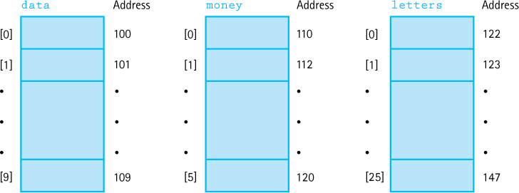
Now we have determined the base address of each array: data is 100, money is 110, and letters is 122. The arrangement of these arrays in memory gives us the following relationships:

In C++ the accessing function that gives us the position of an element in a one-dimensional array associated with the expression Index is
Address(Index) = Base + Offset of the element at position Index
How do we calculate the offset? The general formula is
Offset = Index * SizeOfElement
The whole accessing function becomes
Address(Index) = Base + Index * SizeOfElement
Let’s apply this formula and see if we do get what we claimed we should.
| Base + Index * SizeOfElement | Address | |
|---|---|---|
data[0] |
100 + (0 * 1) |
= 100 |
data[8] |
100 + (8 * 1) |
= 108 |
letters[1] |
122 + (1 * 1) |
= 123 |
letters[25] |
122 + (25 * 1) |
= 147 |
money[0] |
110 + (0 * 2) |
= 110 |
money[3] |
110 + (3 * 2) |
= 116 |
Earlier, we noted that an array is a structured data type. Unlike with a record, whose logical view is unstructured but whose implementation view is structured, both views of an array are structured. The structure is inherent in the logical component selector.
As we mentioned at the beginning of this section, when you use an array in a C++ program you do not have to be concerned with all of these implementation details. The advantages of this approach are very clear: You can think of the data and the operations in a logical sense and can consider their use without having to worry about implementation details. The lower levels are still there—they just remain hidden from you. We strive for this same sort of separation of the abstract and implementation views in the programmer-defined classes discussed in the remainder of this book.
Two-Dimensional Arrays
Logical Level
Most of what we have said about the abstract view of a one-dimensional array applies as well to arrays of more than one dimension. A two-dimensional array is a composite data type made up of a finite, fixed-size collection of homogeneous elements ordered in two dimensions. Its component selector is direct access: a pair of indexes specifies the desired element by giving its relative position in each dimension.
A two-dimensional array is a natural way to represent data that is logically viewed as a table with columns and rows. The following example illustrates the syntax for declaring a two-dimensional array in C++.
int table[10][6];
The abstract picture of this structure is a grid with rows and columns.

The component selector for the two-dimensional array is as follows:
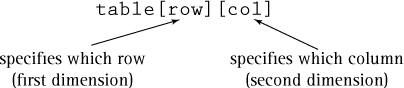
Application Level
As mentioned in the previous section, a two-dimensional array is the ideal data structure for modeling data that are logically structured as a table with rows and columns. The first dimension represents rows, and the second dimension represents columns. Each element in the array contains a value, and each dimension represents a relationship. For example, we usually represent a map as a two-dimensional array.

As with the one-dimensional array, the operations available for a two-dimensional array object are so limited (only creation and direct access) that the major application is the implementation of higher-level objects.
Implementation Level
The implementation of two-dimensional arrays involves the mapping of two indexes to a particular memory cell. The mapping functions are more complicated than those for one-dimensional arrays. We do not give them here, as you will learn to write these accessing functions in later courses. Our goal is not to teach you to be a compiler writer but rather to give you an appreciation of the value of information hiding and encapsulation.
2.3 Higher-Level Abstraction and the C++ Class Type
In the last section, we examined C++’s built-in data types from the logical view, the application view, and the implementation view. Now we shift our focus to data types that are needed in a program but not provided by the programming language.
The class type is a construct in which the members of the class can be both functions and data; that is, the data members and the code that manipulates them are bound together within the class itself. Because the data are bound together with the operations, we can use one object to build another object; in other words, a data member of an object can be another object.
When we design an ADT, we want to bind the operations of the data type with the data that are being manipulated. The class is the perfect mechanism to implement an ADT because it enforces encapsulation3. The class acts like the case around a watch that prevents us from accessing the works. The case is provided by the watchmaker, who can easily open it when repairs become necessary.
Classes are written in two parts, the specification and the implementation. The specification, which defines the interface to the class, is like the face and knobs on a watch. The specification describes the resources that the class can supply to the program. Resources supplied by a watch might include the value of the current time and operations to set the current time. In a class, the resources include data and operations on the data. The implementation section provides the implementation of the resources defined in the specification; it is like the inside of the watch.
Significant advantages are derived from separating the specification from its implementation. A clear interface is important, particularly when a class is used by other members of a programming team or is part of a software library. Any ambiguity in an interface may result in problems. By separating the specification from its implementation, we are given the opportunity to concentrate our efforts on the design of a class without needing to worry about implementation details.
Another advantage of this separation is that we can change the implementation at any time without affecting the programs that use the class (clients of the class). We can make changes when a better algorithm is discovered or the environment in which the program is run changes. For example, suppose we need to control how text is displayed on screen. Text control operations might include moving the cursor to a particular location and setting text characteristics such as bold, blink, and underline. The algorithms required for controlling these characteristics usually differ from one computer system to another. By defining an interface and encapsulating the algorithms as member functions, we can easily move our program to a different system simply by rewriting the implementation. We do not have to change the rest of the program.
Because the class is such an important construct, we review its syntax and semantics in the next section. You should be familiar with most of this material. Indeed, we used a class in Chapter 1.
Class Specification
Although the class specification and implementation can reside in the same file, the two parts of a class are usually separated into two files: The specification goes into a header file (.h extension), and the implementation goes into a file with the same name but a .cpp extension. This physical separation of the two parts of a class reinforces the logical separation.4
We describe the syntax and semantics of the class type within the context of defining an ADT Date.
// Declare a class to represent the Date ADT.
// This is file DateType.h.

class DateType
{
public:
  void Initialize(int newMonth, int newDay, int newYear);
  int GetYear() const;    // Returns year
  int GetMonth() const;   // Returns month
  int GetDay() const;     // Returns day
private:
  int year;
  int month;
  int day;
};
The data members of the class are year, month, and day. The scope of a class includes the parameters on the member functions, so we must use names other than month, year, and day for our formal parameters. The data members are marked private, which means that although they are visible to the human user, they cannot be accessed by client code. Private members can be accessed only by the code in the implementation file.
The member functions of the class are Initialize, GetYear, GetMonth, and GetDay. They are marked public, which means that client code can access these functions. Initialize is a constructor operation; it takes values for the year, month, and day and stores these values into the appropriate data members of an object (an instance of the class).5 GetYear, GetMonth, and GetDay are accessor functions; they are member functions that access the data members of the class. The const beside the accessor function names guarantees that these functions do not change any of the data members of the objects to which they are applied.
Class Implementation
Only the member functions of the class DateType can access the data members, so we must associate the class name with the function definitions. We do so by inserting the class name before the function name, separated by the scope resolution operator (::). The implementation of the member functions goes into the file DateType.cpp. To access the specifications, we must insert the file DateType.h by using an #include directive.
// Define member functions of class DateType.
// This is file DateType.cpp.

#include "DateType.h"     // Gain access to specification of class

void DateType::Initialize
    (int newMonth, int newDay, int newYear)
// Post: year is set to newYear.
//       month is set to newMonth.
//       day is set to newDay.
{
 year = newYear;
 month = newMonth;
 day = newDay;
}

int DateType::GetMonth() const
// Accessor function for data member month.
{
 return month;
}

int DateType::GetYear() const
// Accessor function for data member year.
{
 return year;
}

int DateType::GetDay() const
// Accessor function for data member day.
{
 return day;
}
A client of the class DateType must have an #include "DateType.h" directive for the specification (header) file of the class. Note that system-supplied header files are enclosed in angle brackets (<iostream>), whereas user-defined header files are enclosed in double quotes. The client then declares a variable of type DateType just as it would any other variable.
#include "DateType.h"
DateType today;
DateType anotherDay;
Member functions of a class are invoked in the same way that data members of a struct are accessed—with the dot notation. The following code segment initializes two objects of type DateType and then prints the dates on the screen:
today.Initialize(9, 24, 2003);
anotherDay.Initialize(9, 25, 2003);
cout  << " Today is " << today.GetMonth() << "/" << today.GetDay()
      << "/" << today.GetYear() << endl;
cout  << " Another date is " << anotherDay.GetMonth() << "/"
      << anotherDay.GetDay() << "/" << anotherDay.GetYear() << endl;
Member Functions with Object Parameters
A member function applied to a class object uses the dot notation. What if we want a member function to operate on more than one object—for example, a function that compares the data members of two instances of the class?
Let’s expand our class DateType with a member function ComparedTo that compares two date objects: the instance to which it is applied and its parameter. The function returns LESS if the instance comes before the parameter, EQUAL if they are the same, and GREATER if the instance comes after the parameter. In order to make this work, we must define an enumerated type containing these constants. Here is the enumerated type and the function heading.
The following code compares two instances of the class DateType.
enum RelationType {LESS, EQUAL, GREATER};
// Prototype of member function in the specification file.
RelationType ComparedTo(DateType someDate);
// Compares self with someDate.
To determine which date comes first, we must compare the year members of the instance and the parameter. If they are the same, we must compare the month members. If both the year members and the month members are the same, we must compare the day members. To access the fields of the instance, we just use their name. To access the fields of the parameter, we prefix the field name with the parameter name and a dot. Here, then, is the code for comparedTo.
RelationType DateType::ComparedTo(DateType aDate)
// Pre: Self and aDate have been initialized.
// Post: Function value = LESS, if self comes before aDate.
//                      = EQUAL, if self is the same as aDate.
//                      = GREATER, if self comes after aDate.

{
 if (year < aDate.year)
   return LESS;
 else if (year > aDate.year)
   return GREATER;
 else if (month < aDate.month)
   return LESS;
 else if (month > aDate.month)
   return GREATER;
 else if (day < aDate.day)
   return LESS;
 else if (day > aDate.day)
   return GREATER;
 else return EQUAL;
}
In this code, year refers to the year data member of the object to which the function is applied; aDate.year refers to the data member of the object passed as a parameter.
The object to which a member function is applied is called self. In the function definition, the data members of self are referenced directly without using dot notation. If an object is passed as a parameter, the parameter name must be attached to the data member being accessed using dot notation. As an example, look at the following client code:
switch (today.ComparedTo(anotherDay))
{
  case LESS :
     cout << "today comes before anotherDay";
     break;
  case GREATER :
     cout << "today comes after anotherDay";
     break;
  case EQUAL :
    cout << "today and anotherDay are the same";
    break;
}
Now look back at the ComparedTo function definition. In that code, year in the function refers to the year member of today, and aDate.year in the function refers to the year member of anotherDay, the actual parameter to the function.
Why do we use LESS, GREATER, and EQUAL when COMES_BEFORE, COMES_AFTER, and SAME would be more meaningful in the context of dates? We use the more general words here because in other places we use functions of type RelationType when comparing numbers and strings.
Difference Between Classes and Structs
In C++, the technical difference between classes and structs is that without the use of the reserved words public and private, member functions and data are private by default in classes and public by default in structs. In practice, structs and classes are often used differently. Because the data in a struct are public by default, we can think of a struct as a passive data structure. The operations that are performed on a struct are usually global functions to which the struct is passed as a parameter. Although a struct may have member functions, they are seldom defined. In contrast, a class is an active data structure where the operations defined on the data members are member functions of the class.
In object-oriented programming, an object is viewed as an active structure with control residing in the object through the use of member functions. For this reason, the C++ class type is used to represent the concept of an object.
2.4 Object-Oriented Programming
In Chapter 1, we said that functional design results in a hierarchy of tasks and that object-oriented design results in a hierarchy of objects. Structured programming is the implementation of a functional design, and object-oriented programming (OOP) is the implementation of an object-oriented design. However, these approaches are not entirely distinct: The implementation of an operation on an object often requires a functional design of the algorithm. In this section, we examine object-oriented programming in more depth.
Concepts
The vocabulary of object-oriented programming has its roots in the programming languages Simula and Smalltalk. It can be very bewildering. Such terms and phrases as “sending a message to,” “methods,” and “instance variables” are sprinkled throughout the OOP literature. Although this vocabulary can seem daunting, don’t panic. There is a straightforward translation between these terms and familiar C++ constructs.
An object is a class object or class instance—that is, an instance of a class type. A method is a public member function, and an instance variable is a private data member. Sending a message means calling a public member function. In the rest of this book, we tend to mix object-oriented terms with their C++ counterparts.
There are three basic ingredients in any object-oriented language: encapsulation, inheritance, and polymorphism. We have already discussed encapsulation and how the C++ class construct is designed to encourage encapsulation. In the next two sections we discuss inheritance and polymorphism.
Inheritance
Inheritance is a mechanism whereby a hierarchy of classes is constructed such that each descendant class inherits the properties (data and operations) of its ancestor class. In the world at large, it is often possible to arrange concepts into an inheritance hierarchy—a hierarchy in which each concept inherits the properties of the concept immediately above it in the hierarchy. For example, we might classify different kinds of vehicles according to the inheritance hierarchy in Figure 2.7. Moving down the hierarchy, each kind of vehicle is both more specialized than its parent (and all of its ancestors) and more general than its children (and all of its descendants). A wheeled vehicle inherits properties common to all vehicles (it holds one or more people and carries them from place to place) but has an additional property that makes it more specialized (it has wheels). A car inherits properties common to all wheeled vehicles, but has additional, more specialized properties (four wheels, an engine, a body, and so forth). The inheritance relationship can be viewed as an is-a relationship. In this relationship, the objects become more specialized the lower in the hierarchy you go.

Figure 2.7 Inheritance hierarchy
Object-oriented languages provide a way for creating inheritance relationships among classes. You can take an existing class (called the base class) and create a new class from it (called the derived class). The derived class inherits all the properties of its base class. In particular, the data and operations defined for the base class are now defined for the derived class. Note the is-a relationship—every object of a derived class is also an object of the base class.
Polymorphism
Polymorphism is the ability to determine either statically or dynamically which of several methods with the same name (within the class hierarchy) should be invoked. Overloading means giving the same name to several different functions (or using the same operator symbol for different operations). You have already worked with overloaded operators in C++. The arithmetic operators are overloaded because they can be applied to integral values or floating-point values, and the compiler selects the correct operation based on the operand types. The time at which a function name or symbol is associated with code is called binding time (the name is bound to the code). With overloading, the determination of which particular implementation to use occurs statically (at compile time). Determining which implementation to use at compile time is called static binding.
Dynamic binding, on the other hand, is the ability to postpone the decision of which operation is appropriate until run time. Many programming languages support overloading; only a few, including C++, support dynamic binding. Polymorphism involves a combination of both static and dynamic binding.
Encapsulation, inheritance, and polymorphism are the three necessary constructs in an object-oriented programming language.
C++ Constructs for OOP
In an object-oriented design of a program, classes typically exhibit one of the following relationships: They are independent of one another, they are related by composition, or they are related by inheritance.
Composition
Composition (or containment) is the relationship in which a class contains a data member that is an object of another class type. C++ does not need any special language notation for composition. You simply declare a data member of one class to be of another class type.
For example, we can define a class PersonType that has a data member birthdate of class DateType.
#include <string>
class PersonType

{
public:
 void Initialize(string, DateType);
 string GetName() const;
 DateType GetBirthdate() const;
private:
 string name;
 DateType birthdate;
};
Deriving One Class from Another
Let’s use class PersonType as a base class and derive class StudentType from it with the additional data field status.
class StudentType : public PersonType
{
public:
 string GetStatus() const;
 void Initialize(string, DateType, string);
private:
 string status;
};

StudentType student;
The colon followed by the words public and PersonType (a class identifier) says that the new class being defined (StudentType) is inheriting the members of class PersonType. PersonType is called the base class or superclass and StudentType is called the derived class or subclass.
student has three member variables: one of its own (status) and two that it inherits from PersonType (name and birthdate). student has five member functions: two of its own (Initialize and GetStatus) and three that it inherits from PersonType (Initialize, GetName, and GetBirthdate). Although student inherits the private member variables from its base class, it does not have direct access to them. student must use the public member functions of PersonType to access its inherited member variables.
void StudentType::Initialize
  (string newName, DateType newBirthdate, string newStatus)
{
  status = newStatus;
  PersonType::Initialize(newName, newBirthdate);
}
string StudentType::GetStatus() const

{
 return status;
}
Notice that the scope resolution operator (::) is used between the type PersonType and the member function Initialize in the definition of the member function. Because there are now two member functions named Initialize, one in PersonType and one in StudentType, you must indicate the class in which the one you mean is defined. (That’s why it’s called the scope resolution operator.) If you do not, the compiler assumes you mean the most recently defined one.
The basic C++ rule for passing parameters is that the actual parameter and its corresponding formal parameter must be of an identical type. With inheritance, C++ relaxes this rule somewhat. The type of the actual parameter may be an object of a derived class of the formal parameter.
Remember that inheritance is a logical issue, not an implementation one. A class inherits the behavior of another class and enhances it in some way. Inheritance does not mean inheriting access to another class’s private variables. Although some languages do allow access to the base class’s private members, such access often defeats the concepts of encapsulation and information hiding. With C++, access to the private data members of the base class is not allowed. Neither external client code nor derived class code can directly access the private members of the base class.
Virtual Methods
In the previous section we defined two methods with the same name, Initialize. The statements
person.Initialize("Al", date);
student.Initialize("Al", date, "freshman");
are not ambiguous, because the compiler can determine which Initialize to use by examining the type of the object to which it is applied. There are times, however, when the compiler cannot make the determination of which member function is intended, and the decision must be made at run time. If the decision is to be left until run time, the word virtual must precede the member function heading in the base class definition and a class object passed as a parameter to a virtual function must be a reference parameter. We have more to say about how C++ implements polymorphism when we use it later in the book.
2.5 Constructs for Program Verification
Chapter 1 described methods for verifying software correctness in general. In this section we look at two constructs provided in C++ to help ensure quality software (if we use them!). The first is the exception mechanism, mentioned briefly in Chapter 1. The second is the namespace mechanism, which helps handle the problem of duplicate names appearing in large programs.
Exceptions
Most programs, and student programs in particular, are written under the most optimistic of assumptions: They will compile the first time and execute properly. Such an assumption is far too optimistic for almost any program beyond “Hello world.” Programs must deal with all sorts of error conditions and exceptional situations—some caused by hardware problems, some caused by bad input, and some caused by undiscovered bugs.
Aborting the program in the wake of such errors is not an option, as the user would lose all work performed since the last save. At a minimum, a program must warn the user, allow saving, and exit gracefully. In each situation, even if the exception management technique calls for terminating the program, the code detecting the error cannot know how to shut down the program, let alone shut it down gracefully. Transfer of the thread of control and information to a handler that knows how to manage the error situation is essential.
As we said in Chapter 1, working with exceptions begins at the design phase, where the unusual situations and possible error conditions are specified and decisions are made about handling each one. Now let’s look at the try-catch and throw statements, which allow us to alert the system to an exception (throw the exception), to detect an exception (try code with a possible exception), and to handle an exception (catch the exception).
try-catch and throw Statements
The code segment in which an exception might occur is enclosed within the try clause of a try-catch statement. If the exception occurs, the reserved word throw is used to alert the system that control should pass to the exception handler. The exception handler is the code segment in the catch clause of the associated try-catch statement, which takes care of the situation.
The code that may throw an exception is placed in a try block followed immediately by one or more catch blocks. A catch block consists of the keyword catch followed by an exception declaration, which is in turn followed by a block of code. If an exception is thrown, execution immediately transfers from the try block to the catch block whose type matches the type of the thrown exception. The exception variable receives the exception of the type that is thrown in the try block. In this way, the thrown exception communicates information about the event to the handler.
try
{
 // Code that may raise an exception and/or set some condition
 if (condition)
   throw exception_name; // frequently a string
}
catch (typename variable)
{
 // Code that handles the exception
 // It may call a cleanup routine and exit if the
 // program must be terminated
}

// Code to continue processing
//   This will be executed unless the catch block
//   stops the processing.
Let’s look at a concrete example. You are reading and summing positive values from a file. An exception occurs if a negative value is encountered. If this event happens, you want to write a message to the screen and stop the program.
try
{
  infile >> value;
  do
  {
    if (value < 0)
      throw string("Negative value"); // Exception is a string
    sum = sum + value;
  } while (infile);
}
catch (string message)
// Parameter of the catch is type string
{
  // Code that handles the exception
  cout << message << " found in file. Program aborted."
  return 1;
}
// Code to continue processing if exception not thrown
cout << "Sum of values on the file: " << sum;
If value is less than zero, a string is thrown; catch has a string as a parameter. The system recognizes the appropriate handler by the type of the exception and the type of the catch parameter. We will deal with exceptions throughout the rest of the book. As we do, we will show more complex uses of the try-catch statement.
Here are the rules we follow in using exceptions within the context of the ADTs we develop:
The preconditions/postconditions on the functions represent a contract between the client and the ADT that defines the exception(s) and specifies who (client or ADT) is responsible for detecting the exception(s).
The client is always responsible for handling the exception.
The ADT code does not check the preconditions.
When we design an ADT, the software that uses it is called the client of the class. In our discussion, we use the terms client and user interchangeably, thinking of them as the people writing the software that uses the class, rather than the software itself.
Standard Library Exceptions
In C++, the run-time environment (for example, a divide-by-zero error) may implicitly generate exceptions in addition to those being thrown explicitly by the program. The standard C++ libraries provide a predefined hierarchy of error classes in the standard header file, stdexcept, including
logic_errordomain_errorinvalid_argumentlength_errorout_of_range
In addition, the class runtime_error provides the following error classes:
range_erroroverflow_errorunderflow_error
Namespaces
Different code authors tend to use many of the same identifier names (name, for example). Because library authors often have the same tendency, some of these names may appear in the library object code. If these libraries are used simultaneously, name clashes may occur, as C++ has a “one definition rule,” which specifies that each name in a C++ program should be defined exactly once. The effect of dumping many names into the namespace is called namespace pollution.
The solution to namespace pollution involves the use of the namespace mechanism. A namespace is a C++ language technique for grouping a collection of names that logically belong together. This facility allows the enclosing of names in a scope that is similar to a class scope; unlike class scope, however, a namespace can extend over several files and be broken into pieces in a particular file.
Creating a Namespace
A namespace is declared with the keyword namespace before the block that encloses all of the names to be declared within the space. To access variables and functions within a namespace, place the scope resolution operator (::) between the namespace name and the variable or function name. For example, if we define two namespaces with the same function,
namespace myNames
{
  void GetData(int&);
};

namespace yourNames
{
  void GetData(int&);
};
you can access the functions as follows:
myNames::GetData(int& dataValue);        // GetData from myNames
yourNames::GetData(int& dataValue); // GetData from yourNames
This mechanism allows identical names to coexist in the same program.
Access to Identifiers in a Namespace
Access to names declared in a namespace may always be obtained by explicitly qualifying the name with the name of the namespace with the scope resolution operator (::), as shown in the last example. Explicit qualification of names is sufficient to use these names. However, if many names will be used from a particular namespace or if one name is used frequently, then repeated qualification can be awkward. A using declaration avoids this repetition for a particular identifier. The using declaration creates a local alias for the qualified name within the block in which it is declared, making qualification unnecessary.
For example, by putting the following declaration in the program,
using myNames::GetData;
the function GetData can be used subsequently without qualification. To access GetData in the namespace yourNames, it would have to be qualified: yourNames::GetData.
One other method of access should be familiar: a using directive. For example,
using namespace myNames;
provides access to all identifiers within the namespace myNames. You undoubtedly have employed a using directive in your program to access cout and cin defined in the namespace std without having to qualify them.
A using directive does not bring the names into a given scope; rather, it causes the name-lookup mechanism to consider the additional namespace specified by the directive. The using directive is easier to use, but it makes a large number of names visible in this scope and can lead to name clashes.
Rules for Using the Namespace std
Here are the rules that we follow in the balance of the text in terms of qualifying identifiers from the namespace std:
In function prototypes and/or function definitions, we qualify the identifier in the heading.
In a function block, if a name is used once, it is qualified. If a name is used more than once, we use a using declaration with the name.
If two or more names are used from a namespace, we use a using directive.
A using directive is never used outside a class or a function block.
The goal is to never pollute the global namespace more than is necessary.
2.6 Comparison of Algorithms
There is more than one way to solve most problems. If you were asked for directions to Joe’s Diner (see Figure 2.8), you could give either of two equally correct answers:
“Go east on the big highway to the Y’all Come Inn, and turn left.”
“Take the winding country road to Honeysuckle Lodge, and turn right.”
The two answers are not the same, but following either route gets the traveler to Joe’s Diner. Thus both answers are functionally correct.
If the request for directions contained special requirements, one solution might be preferable to the other. For instance, “I’m late for dinner. What’s the quickest route to Joe’s Diner?” calls for the first answer, whereas “Is there a pretty road that I can take to get to Joe’s Diner?” suggests the second. If no special requirements are known, the choice is a matter of personal preference—which road do you like better?

Figure 2.8 Map to Joe’s Diner
How we choose between two algorithms that perform the same task often depends on the requirements of a particular application. If no relevant requirements exist, the choice may be based on the programmer’s own style.
Often the choice between algorithms comes down to a question of efficiency. Which one takes the least amount of computing time? Which one does the job with the least amount of work? We are talking here of the amount of work that the computer does. Later we also compare algorithms in terms of how much work the programmer does. (One is often minimized at the expense of the other.)
To compare the work done by competing algorithms, we must first define a set of objective measures that can be applied to each algorithm. The analysis of algorithms is an important area of theoretical computer science; in advanced courses, students undoubtedly see extensive work in this area. In this book, you learn about a small part of this topic, enough to let you determine which of two algorithms requires less work to accomplish a particular task.
How do programmers measure the work performed by two algorithms? The first solution that comes to mind is simply to code the algorithms and then compare the execution times for running the two programs. The one with the shorter execution time is clearly the better algorithm. Or is it? Using this technique, we can determine only that program A is more efficient than program B on a particular computer. Execution times are specific to a particular machine. Of course, we could test the algorithms on all possible computers, but we want a more general measure.
A second possibility is to count the number of instructions or statements executed. This measure, however, varies with the programming language used as well as with the individual programmer’s style. To standardize this measure somewhat, we could count the number of passes through a critical loop in the algorithm. If each iteration involves a constant amount of work, this measure gives us a meaningful yardstick of efficiency.
Another idea is to isolate a particular operation fundamental to the algorithm and count the number of times that this operation is performed. Suppose, for example, that we are summing the elements in an integer list. To measure the amount of work required, we could count the integer addition operations. For a list of 100 elements, there are 99 addition operations. Note, however, that we do not actually have to count the number of addition operations; it is some function of the number of elements (N) in the list. Therefore, we can express the number of addition operations in terms of N: For a list of N elements, N – 1 addition operations are carried out. Now we can compare the algorithms for the general case, not just for a specific list size.
If we wanted to compare algorithms for summing and counting a list of real numbers we could use a measure that combines the real multiplication and integer increment operations required. This example brings up an interesting consideration: Sometimes an operation so dominates the algorithm that the other operations fade into the background “noise.” If we want to buy elephants and goldfish, for example, and we are considering two pet suppliers, we need to compare only the prices of elephants; the cost of the goldfish is trivial in comparison. Similarly, on many computers floating-point addition is so much more expensive than integer increment in terms of computer time that the increment operation is a trivial factor in the efficiency of the whole algorithm; we might as well count only the addition operations and ignore the increments. In analyzing algorithms, we often can find one operation that dominates the algorithm, effectively relegating the others to the “noise” level.

Big-O
We have talked about work as a function of the size of the input to the operation (for instance, the number of elements in the list to be summed). We can express an approximation of this function using a mathematical notation called order of magnitude, or Big-O notation. (This is the letter O, not a zero.) The order of magnitude of a function is identified with the term in the function that increases fastest relative to the size of the problem. For instance, if
f(N) = N4 + 100N2 + 10N + 50
then f (N) is of order N 4—or, in Big-O notation, O(N 4). That is, for large values of N, some multiple of N 4 dominates the function for sufficiently large values of N.
Why can we just drop the low-order terms? Remember the elephants and goldfish that we discussed earlier? The price of the elephants was so much greater that we could just ignore the price of the goldfish. Similarly, for large values of N, N 4 is so much larger than 50, 10N, or even 100N2 that we can ignore these other terms. This doesn’t mean that the other terms do not contribute to the computing time, but rather that they are not significant in our approximation when N is “large.”
What is this value N? N represents the size of the problem. Most of the rest of the problems in this book involve data structures—lists, stacks, queues, and trees. Each structure is composed of elements. We develop algorithms to add an element to the structure and to modify or delete an element from the structure. We can describe the work done by these operations in terms of N, where N is the number of elements in the structure. Yes, we know. We have called the number of elements in a list the length of the list. However, mathematicians talk in terms of N, so we use N for the length when we are comparing algorithms using Big-O notation.
Suppose that we want to write all the elements in a list into a file. How much work is involved? The answer depends on how many elements are in the list. Our algorithm is
If N is the number of elements in the list, the “time” required to do this task is
(N * time-to-write-one-element) + time-to-open-the-file
This algorithm is O(N) because the time required to perform the task is proportional to the number of elements (N)—plus a little time to open the file. How can we ignore the open time in determining the Big-O approximation? Assuming that the time necessary to open a file is constant, this part of the algorithm is our goldfish. If the list has only a few elements, the time needed to open the file may seem significant. For large values of N, however, writing the elements is an elephant in comparison with opening the file.
The order of magnitude of an algorithm does not tell you how long in microseconds the solution takes to run on your computer. Sometimes we need that kind of information. For instance, a word processor’s requirements may state that the program must be able to spell-check a 50-page document (on a particular computer) in less than 2 seconds. For such information, we do not use Big-O analysis; we use other measurements. We can compare different implementations of a data structure by coding them and then running a test, recording the time on the computer’s clock before and after the test. This kind of “benchmark” test tells us how long the operations take on a particular computer, using a particular compiler. The Big-O analysis, however, allows us to compare algorithms without reference to these factors.
Common Orders of Magnitude
O(1) is called bounded time. The amount of work is bounded by a constant and does not depend on the size of the problem. Assigning a value to the ith element in an array of N elements is O(l), because an element in an array can be accessed directly through its index. Although bounded time is often called constant time, the amount of work is not necessarily constant. Rather, it is bounded by a constant.
O(log2N) is called logarithmic time. The amount of work depends on the log of the size of the problem. Algorithms that successively cut the amount of data to be processed in half at each step typically fall into this category. Finding a value in a list of ordered elements using the binary search algorithm is O(log2N).
O(N) is called linear time. The amount of work is some constant times the size of the problem. Printing all the elements in a list of N elements is O(N). Searching for a particular value in a list of unordered elements is also O(N), because you (potentially) must search every element in the list to find it.
O(N log2N) is called (for lack of a better term) N log2N time. Algorithms of this type typically involve applying a logarithmic algorithm N times. The better sorting algorithms, such as Quicksort, Heapsort, and Mergesort discussed in later chapters, have N log2N complexity. That is, these algorithms can transform an unordered list into a sorted list in O(N log2N) time.
O(N 2) is called quadratic time. Algorithms of this type typically involve applying a linear algorithm N times. Most simple sorting algorithms are O(N 2) algorithms.
O(N 3) is called cubic time. An example of an O(N 3) algorithm is a routine that increments every element in a three-dimensional table of integers.
O(2N) is called exponential time. These algorithms are costly. As you can see in Table 2.1, exponential times increase dramatically in relation to the size of N. (Note that the values in the last column grow so quickly that the computation time required for problems of this order may exceed the estimated life span of the universe!)
Example 1: Sum of Consecutive Integers
Throughout this discussion we have been talking about the amount of work the computer must do to execute an algorithm. This determination does not necessarily relate to the size of the algorithm, say, in lines of code. Consider the following two algorithms to initialize to zero every element in an N-element array:
Algorithm Init1               Algorithm Init2
items[0]  = 0;                for (index = 0; index < N; index++)
items[1]  = 0;                  items[index] = 0;
items[2]  = 0;
items[3]  = 0;
          .
          .
          .
items[N – 1]  = 0;
Both algorithms are O(N), even though they greatly differ in the number of lines of code.
Table 2.1 Comparison of Rates of Growth
| N | log2 N | N log2N | N2 | N3 | 2N |
|---|---|---|---|---|---|
| 1 | 0 | 1 | 1 | 1 | 2 |
| 2 | 1 | 2 | 4 | 8 | 4 |
| 4 | 2 | 8 | 16 | 64 | 16 |
| 8 | 3 | 24 | 64 | 512 | 256 |
| 16 | 4 | 64 | 256 | 4,096 | 65,536 |
| 32 | 5 | 160 | 1,024 | 32,768 | 4,294,967,296 |
| 64 | 6 | 384 | 4,096 | 262,114 | About ten minute’s worth of instructions on a super-computer |
| 128 | 7 | 896 | 16,384 | 2,097,152 | About 7.8 × 10¹¹ times greater than the age of the universe in nanoseconds (for a 13.8-billion-year estimate) |
| 256 | 8 | 2,048 | 65,536 | 16,777,216 | Don’t ask! |
Now let’s look at two different algorithms that calculate the sum of the integers from 1 to N. Algorithm Suml is a simple for loop that adds successive integers to keep a running total:
Algorithm Sum1
sum = 0;
for (count = 1; count <= n; count++)
   sum = sum + count;
That seems simple enough. The second algorithm calculates the sum by using a formula. To understand the formula, consider the following calculation when N = 9:
  1 +  2 +  3 +  4 +  5 +  6 +  7 +  8 +  9
+ 9 +  8 +  7 +  6 +  5 +  4 +  3 +  2 +  1
_____________________________________________________________
 10 + 10 + 10 + 10 + 10 + 10 + 10 + 10 + 10 =   10 * 9 = 90
We pair up each number from 1 to N with another, such that each pair adds up to N + 1. There are N such pairs, giving us a total of (N + 1) * N. Now, because each number is included twice, we divide the product by 2. Using this formula, we can solve the problem: ((9 + 1) * 9)/2 = 45. Now we have a second algorithm:
Algorithm Sum2
sum = ((n + 1) * n) / 2;
Both of the algorithms are short pieces of code. Let’s compare them using Big-O notation. The work done by Sum1 is a function of the magnitude of N; as N gets larger, the amount of work grows proportionally. If N is 50, Sum1 works 10 times as hard as when N is 5. Algorithm Sum1, therefore, is O(N).

To analyze Sum2, consider the cases when N = 5 and N = 50. They should take the same amount of time. In fact, whatever value we assign to N, the algorithm does the same amount of work to solve the problem. Algorithm Sum2, therefore, is O(1).
Is Sum2 always faster? Is it always a better choice than Sum1? That depends. Sum2 might seem to do more “work,” because the formula involves multiplication and division, whereas Sum1 calculates a simple running total. In fact, for very small values of N, Sum2 actually might do more work than Suml. (Of course, for very large values of N, Suml does a proportionally larger amount of work, whereas Sum2 stays the same.) So the choice between the algorithms depends in part on how they are used, for small or large values of N.
Another issue is the fact that Sum2 is not as obvious as Suml, and thus it is more difficult for the programmer (a human) to understand. Sometimes a more efficient solution to a problem is more complicated; we may save computer time at the expense of the programmer’s time.
What’s the verdict? As usual in the design of computer programs, there are tradeoffs. We must look at our program’s requirements and then decide which solution is better.
Example 2: Finding a Number in a Phone Book
Suppose you need to look up a friend’s number in a phone book. How would you go about finding the number? To keep matters simple, assume that the name you are searching for is in the book—you won’t come up empty. Here is a straightforward approach.
Even though this algorithm is inefficient, it is correct and does work.
What is the Big-O efficiency rating of this algorithm? How many steps does it take to find someone’s name? Clearly the answers to these questions depend on the size of the phone book and the name that you are searching for. If you are looking for your friend Aaron Aardvark, it probably takes you only one or two steps. If your friend’s name is Zina Zyne, you are not so lucky.
The Lookup1 algorithm displays different efficiency ratings under different input conditions. This is not unusual. To handle this situation, analysts define three complexity cases: best case, worst case, and average case. Best case complexity tells us the complexity when we are very lucky; it represents the smallest number of steps that an algorithm can take. In general, best case complexity is not very useful as a complexity measure. Worst case complexity, by contrast, represents the greatest number of steps that an algorithm would require. Average case complexity represents the average number of steps required, considering all possible inputs.
Let’s evaluate Lookup1 in each of these cases. Following our previous convention we label the size of our phone book N. Our fundamental operation is “checking a name.”
Best case The name we are looking for is the first name in the phone book, so it takes us only one step to find the name. The best case Big-O complexity of the algorithm is constant or O(1).
Worst case The name we are looking for is the last name in the phone book, so it takes us N steps to find the name. The worst case Big-O complexity of the algorithm is O(N).
Average case Assuming that each name in the phone book is equally likely to be the name we are searching for, the average number of steps required is N/2. Sometimes the name is toward the front of the book, and sometimes it is toward the back of the book. On the average, it is in the middle of the book—thus N/2 steps. The average case Big-O complexity of the algorithm is also O(N).
The average case analysis is usually the most difficult. Often, as in this example, it evaluates to the same Big-O efficiency class as the worst case. For our purposes we will typically use worst case analysis.
Let’s look at a more efficient algorithm for finding a name in a phone book.
With this algorithm we eliminate half of the remaining phone book from consideration each time we check a name. What is the worst case complexity? Another way of asking this is to say, “How many times can you reduce N by half, before you get down to 1?” This is essentially the definition of log2N. Thus the worst case complexity of Lookup2 is O(log2N). This is significantly better than the worst case for Lookup1. For example, if each of New York City’s 8.5 million people were listed in your phone book, then in the worst case Lookup1 would take you 8,500,000 steps, but Lookup2 would require only 24 steps.
Note that the successful use of the Lookup2 algorithm depends on the fact that the phone book organizes names in alphabetical order. This is a good example of a situation in which the way the data are structured and organized affects the efficiency of our use of the data.

Throughout this text we examine different choices of algorithms and data structures. We compare them using Big-O, but we also examine the program’s requirements and the “elegance” of the competing solutions. As programmers, we design software solutions with many factors in mind.
Summary
We have discussed how data can be viewed from multiple perspectives, and we have seen how C++ encapsulates the implementations of its predefined types and allows us to encapsulate our own class implementations.
As we create data structures, using built-in data types such as arrays, structs, and classes to implement them, we see that there are actually many levels of data abstraction. The abstract view of an array might be viewed as the implementation level of the programmer-defined data type List, which uses an array to hold its elements. At the logical level, we do not access the elements of List through their array indexes but rather through a set of accessing operations defined especially for objects of the List type. A data type that is designed to hold other objects is called a container or collection type. Moving up a level, we might see the abstract view of List as the implementation level of another programmer-defined data type, ProductInventory, and so on.

What do we gain by separating these views of the data? First, we reduce complexity at the higher levels of the design, making the program easier to understand. Second, we make the program more easily modifiable: The implementation can be completely changed without affecting the program that uses the data structure. We take advantage of this ability in this text, developing various implementations of the same objects in different chapters. Third, we develop software that is reusable: The structure and its accessing operations can be used by other programs, for completely different applications, as long as the correct interfaces are maintained. You saw in Chapter 1 that the design, implementation, and verification of high-quality computer software is a very laborious process. Being able to reuse pieces that are already designed, coded, and tested cuts down on the amount of work required.
In the chapters that follow, we extend these ideas to build other container classes that C++ does not provide: lists, stacks, queues, priority queues, trees, graphs, and sets. We consider these data structures from the logical view: What is our abstract picture of the data, and what accessing operations can we use to create, assign, and manipulate elements in the data structure? We express our logical view as an ADT and record its description in a data specification.
Next, we take the application view of the data, using an instance of the data type in a short example.
Finally, we change hats and turn to the implementation view of the data type. We consider the C++ type declarations that represent the data structure as well as the design of the functions that implement the specifications of the abstract view. Data structures can be implemented in more than one way, so we often look at alternative representations and methods for comparing them. In some of the chapters, we include a longer Case Study in which instances of the data type are used to solve a problem.
Exercises
-
Explain what we mean by “data abstraction.”
-
What is data encapsulation? Explain the programming goal “to protect our data abstraction through encapsulation.”
-
Name three perspectives from which we can view data. Using the logical data structure “a list of student academic records,” give examples of what each perspective might tell us about the data.
-
Consider the ADT GroceryStore.
At the application level, describe GroceryStore.
At the logical level, what grocery store operations might be defined for the customer?
Specify (at the logical level) the operation CheckOut.
Write an algorithm (at the implementation level) for the operation CheckOut.
Explain how parts (c) and (d) represent information hiding.
-
What composite types are predefined in the C++ language?
-
Describe the component selectors for structs and classes at the logical level.
-
Describe the accessing functions for structs and classes at the implementation level.
-
Describe the component selectors for one-dimensional arrays at the logical level.
-
Describe the accessing functions for one-dimensional arrays at the implementation level.
-
Declare a one-dimensional array,
name, that contains 20 characters.If each character occupies one “cell” in memory, and the base address of
nameis 1000, what is the address of the cell referenced in the following statement?name[9] = 'A';
Use the following declarations for Exercises 11 and 12:
enum MonthType {JAN, FEB, MAR, APR, MAY, JUN, JUL, AUG, SEP,
                OCT, NOV, DEC};
struct WeatherType
{
  int avgHiTemp;
  int avgLoTemp;
  float actualRain;
  float recordRain;
};
Assume that an
intrequires one cell in memory, that afloatnumber requires two cells, and that the struct members are found in contiguous memory locations with no gaps.
-
Declare a one-dimensional array type,
WeatherListType, ofWeatherTypecomponents, to be indexed by values of typeMonthType. Declare a variable,yearlyWeather, ofWeatherListType.Assign the value 1.05 to the actual rainfall member of the July record in
yearlyWeather.If the base address of
yearlyWeatheris 200, what is the address of the member that you assigned in part (b)?
-
Declare a two-dimensional array,
decadeWeather, ofWeatherTypecomponents, to be indexed by values of typeMonthTypein the first dimension.Draw a picture of
decadeWeather.Assign the value 26 to the
avgLoTempmember of the March 2006 entry.
-
Define a three-dimensional array at the logical level.
Suggest some applications for three-dimensional arrays.
Use the following declarations for Exercises 14–16.
typedef char String[10];
struct StudentRecord
{
  String firstName;
  String lastName;
  int id;
  float gpa;
  int currentHours;
  int totalHours;
};
StudentRecord student;
StudentRecord students[100];
Assume that an
intrequires one cell in memory, that afloatnumber requires two cells, and that the struct members are found in contiguous memory locations with no gaps.
-
Construct a member-length-offset table for
StudentRecord. -
If the base address of
studentis 100, what address does the compiler generate as the target of the following assignment statement?student.gpa = 3.87;
-
How much space does the compiler set aside for
students? -
Indicate which predefined C++ types would most appropriately model each of the following (more than one may be appropriate for each):
a chessboard
information about a single product in an inventory-control program
a list of famous quotations
the casualty figures (number of deaths per year) for highway accidents in Texas from 1995 to 2005
the casualty figures for highway accidents in each of the states from 1995 to 2005
the casualty figures for highway accidents in each of the states from 1995 to 2005, subdivided by month
an electronic address book (name, address, and phone information for all your friends)
a collection of hourly temperatures for a 24-hour period
-
What C++ construct is used to represent ADTs?
-
Explain the difference between a C++ struct and class.
-
How is the client prevented from directly accessing the details of an instance of a class?
-
The details of a private member can be seen by the user of a class. (True or False?)
The details of a private member may be accessed by a client program. (True or False?)
-
Why is it good practice to put a class declaration in one file and the implementation in another?
-
Name three ways that classes can relate to each other.
-
Distinguish between composition and inheritance.
-
Distinguish between a base class and a derived class.
-
Does a derived class have access to the private data members of the base class?
-
Does a derived class have access to the public member functions of the base class?
-
Write the specification for an ADT SquareMatrix. (A square matrix can be represented by a two-dimensional array with N rows and N columns.) You may assume a maximum size of 50 rows and columns. Include the following operations:
MakeEmpty(n), which sets the first n rows and columns to zero
StoreValue(i, j, value), which stores a value into the [i, j] position
Add, which adds two matrices together
Subtract, which subtracts one matrix from another
Copy, which copies one matrix into another
Convert your specification to a C++ class declaration.
Implement the member functions.
Write a test plan for your class.
-
DateTypekeeps only the integer representation of the month, day, and year. When a month is wanted in string form, the string is calculated. An alternate approach would be to add a string field to the date and calculate and store the string representation in theInitializefunction. Which methods would have to be changed? Would this change make the use of an if statement to find the appropriate string more or less attractive? Write the code for this if statement. -
What changes would be necessary if the number of days in the month were carried as a data field in class
DateTyperather than being looked up when necessary? Would this change make the use of a switch statement to find the number of days in the month more attractive? Write the code for thisswitchstatement. -
Compare and contrast the implementation of class
DateTypeused in the Case Study and the solution proposed in Exercises 29 and 30. These two approaches represent the classic trade-off between space and algorithm complexity. Please comment.Use the following possible answers for Exercises 32–36.
O(1)
O(logN)
O(N)
O(N logN)
O(N*N)
O(N*N*N)
-
The order of sorting an array of N items using one of the better sorting algorithms such as Quicksort.
-
The order of sorting an array of N items using one of the slower sorting algorithms such as SelectionSort.
-
The order of an algorithm that decrements every element in a three-dimensional table of N rows.
-
The order of an algorithm that increments every element in a two-dimensional table of N rows.
-
The order of comparing three items.
-
True or False? O(N) is called linear time.
-
True or False? O(N) is called log time.
-
True or False? O(N*N) is called quadratic time.
-
True or False? O(1) is called constant time.
-
True or False? An algorithm that has complexity O(logN) is always faster than one that has O(N) complexity.