I search for the realness, the real feeling of a subject, all the texture around it…I always want to see the third dimension of something…I want to come alive with the object.
Andrew Wyeth (1917–2009), American painter, known for “Christina’s World” (1948)
Although two objects might have the same fractal dimension, their structure might be statistically very different. … Instead of only defining the percentage of space not occupied by the structure, lacunarity is more interested in the holes and their distribution on the object under observation. In the case of fractals, even if two fractal objects have the d B, they could have different lacunarity if the fractal “pattern” is different.
 .
.
Cantor dust lacunarity
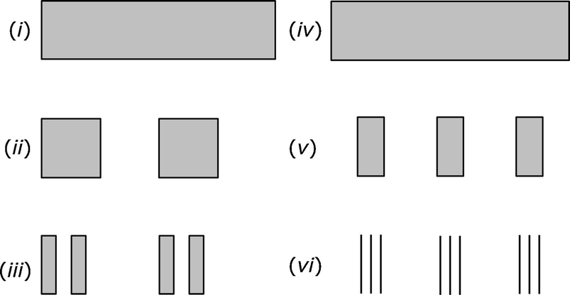
For the second example, we start with the rectangle (iv) which is identical to rectangle (i). We divide rectangle (iv) into nine equal size pieces, and keep only the second, fifth, and eight pieces, discarding the other six pieces, yielding (v). Each piece in (v) is then divided into nine equal size pieces, and we keep only the second, fifth, and eight pieces, discarding the other six pieces, yielding (vi). If we continue this process indefinitely, the resulting fractal has similarity dimension  . So both Cantor dust fractals have d
S = 1∕2 yet they have different textures: the first fractal has a more lumpy texture than the second. The difference in textures is captured using the lacunarity measure. High lacunarity means the object is “heterogeneous”, with a wide range of “gap” or “hole” sizes. Low lacunarity means the object is “homogeneous”, with a narrow range of gap sizes [Plotnick 93]. The value of lacunarity is that the fractal dimension, by itself, has been deemed insufficient to describe some geometric patterns.
. So both Cantor dust fractals have d
S = 1∕2 yet they have different textures: the first fractal has a more lumpy texture than the second. The difference in textures is captured using the lacunarity measure. High lacunarity means the object is “heterogeneous”, with a wide range of “gap” or “hole” sizes. Low lacunarity means the object is “homogeneous”, with a narrow range of gap sizes [Plotnick 93]. The value of lacunarity is that the fractal dimension, by itself, has been deemed insufficient to describe some geometric patterns.
 , independent of k. Yet the distribution of “white space” within these figures varies widely. This is illustrated in Fig. 19.2 where the unit interval is divided into Sixteen pieces, and three constructions are illustrated, one for k = 1 and two for k = 2. The two k = 2 constructions demonstrate that the construction need not be symmetric.
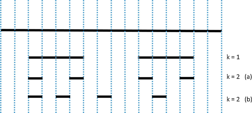
Lacunarity for a Cantor set
The fact that both a solid object in  and a Poisson point pattern in
  have the same d
B illustrates the need to provide a measure of clumpiness [Halley 04]. Methods for calculating lacunarity were proposed in [Mandelbrot 83b], and subsequently other methods were proposed by other researchers. It was observed in [Theiler 88] that “there is no generally accepted definition of lacunarity, and indeed there has been some controversy over how it should be measured”. Sixteen years later, [Halley 04] wrote that “a more precise definition of lacunarity has been problematic”, and observed that at least six different algorithms have been proposed for measuring the lacunarity of a geometric object, and a comparison of four of the six methods showed little agreement among them.
have the same d
B illustrates the need to provide a measure of clumpiness [Halley 04]. Methods for calculating lacunarity were proposed in [Mandelbrot 83b], and subsequently other methods were proposed by other researchers. It was observed in [Theiler 88] that “there is no generally accepted definition of lacunarity, and indeed there has been some controversy over how it should be measured”. Sixteen years later, [Halley 04] wrote that “a more precise definition of lacunarity has been problematic”, and observed that at least six different algorithms have been proposed for measuring the lacunarity of a geometric object, and a comparison of four of the six methods showed little agreement among them.
 . For r > 0, define Φ(r) by
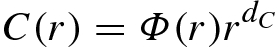
 . The term “lacunarity” was used in [Theiler 88] to refer to the variability in Φ(r), particularly where limr→0Φ(r) is not a positive constant.
19.1 Gliding Box Method
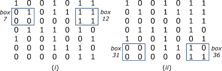
Gliding box method for the top row
Gliding box example continued
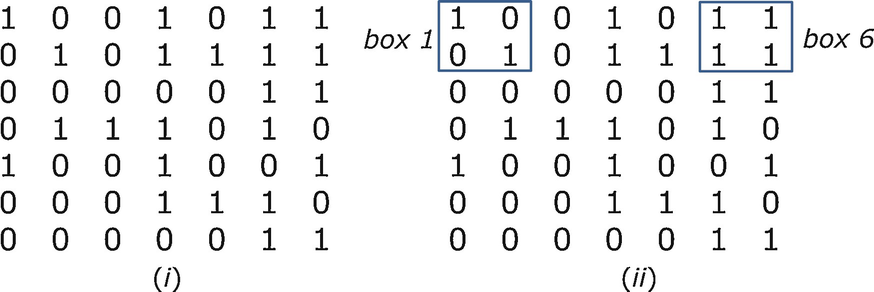
Suppose the matrix has M rows and M columns. An individual box corresponds to the triplet (i, j, s), where the upper left-hand corner of the box is element (i, j) of the matrix, and s is the box size. The range of s is 1 to M. The range of i and j is 1 to M − s + 1, so the total number of boxes of size s is (M − s + 1)2. Let x(i, j, s) be the sum of the matrix entries in the box (i, j, s). In our example we have x(1, 1, 2) = 2, x(1, 6, 2) = 4, x(2, 1, 2) = 1, x(2, 6, 2) = 4, x(6, 1, 2) = 0, and x(6, 6, 2) = 3. For a given s and for k = 0, 1, 2, …, s
2, let N
s(k) be the number of boxes of size s for which x(i, j, s) = k. Since the total number of boxes of size s is (M − s + 1)2 then  .
.


![$$\displaystyle \begin{aligned} \begin{array}{rcl} \varLambda(s) \equiv \frac{\mu_{{\, 2}}(s)}{ [\mu_{{\, 1}}(s)]^2} \, . {} \end{array} \end{aligned} $$](../images/487758_1_En_19_Chapter/487758_1_En_19_Chapter_TeX_Equ3.png)
 . Using the well-known relationship μ
2(s) = [μ
1(s)]2 + σ
2(s) for a probability distribution, we obtain
. Using the well-known relationship μ
2(s) = [μ
1(s)]2 + σ
2(s) for a probability distribution, we obtain ![$$\displaystyle \begin{aligned} \begin{array}{rcl} \varLambda(s) = \frac{ [\mu_{{\, 1}}(s)]^2 + \sigma^2(s) }{ [ \mu_{{\, 1}}(s) ]^2} = \frac{ \sigma^2(s) }{ [ \mu_{{\, 1}}(s) ]^2} + 1 \, . {} \end{array} \end{aligned} $$](../images/487758_1_En_19_Chapter/487758_1_En_19_Chapter_TeX_Equ4.png)
- 1.
From (19.4) we see that Λ(s) ≥ 1 for all s. Moreover, for any totally regular array (e.g., an alternating pattern of 0’s and 1’s), if s is at least as big as the unit size of the repeating pattern, then the x(i, j, s) values are independent of the position (i, j) of the box, which implies μ 2(s) = 0 and hence Λ(s) = 1 [Plotnick 93].
- 2.
Since there is only one box of size M then there is at most one k value for which p M(k) is nonzero, namely, k = x(1, 1, M). Thus the variance of the distribution
 is 0 and from (19.4) we have Λ(M) = 1.
 - 3.
Suppose each of the M 2 elements in the array is 1 with probability p = 1∕M 2. For a box size of 1, the expected number of boxes containing a “1” is pM 2, so from (19.1) we have p 1(1) = pM 2∕M 2 = p. From (19.2) we have μ 1(1) = μ 2(1) = p. Hence Λ(1) = μ 2(1)∕[μ 1(1)]2 = 1∕p [Plotnick 93].
- 4.
Since x(i, j, s) is the sum of the matrix entries in the box (i, j, s), then x(i, j, s) is a non-decreasing function of s, and hence μ 1(s) is also non-decreasing in s. Since the relative variance (i.e., the ratio σ 2(s)∕μ 1(s)) of the x(i, j, s) values is a non-decreasing function of s, then Λ(s) is a non-increasing function of s. Or, as expressed in [Krasowska 04], as s increases, the average mass of the box increases, which increases the denominator μ 1(s) in (19.3); also as s increases the variance μ 2(s) in (19.3) decreases since all features become averaged into “a kind of noise”. Thus Λ(s) decreases as s increases.
- 5.
For a given s, as the mean number of “occupied sites” (i.e., entries in the matrix with the value 1) decreases to zero, the lacunarity increases to ∞ [Plotnick 93]. Thus, for a given s, sparse objects have higher lacunarity than dense objects.
- 6.
The numerical value of Λ(s) for a single value of s is “of limited value at best, and is probably meaningless as a basis of comparison of different maps”. Rather, more useful information can be gleaned by calculating Λ(s) over a range of s [Plotnick 93].
- 7.
For a monofractal in
 , a plot of
  versus
  is a straight line with slope d
B − E [Halley 04].
is a straight line with slope d
B − E [Halley 04].
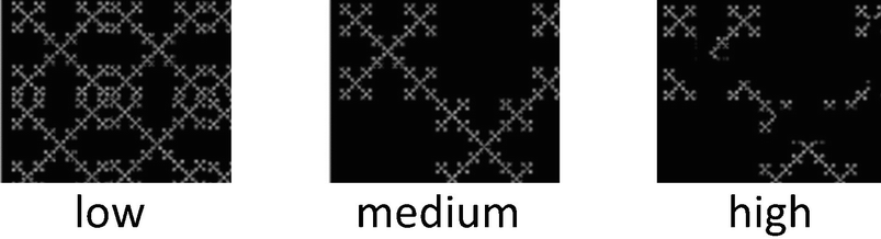
Three degrees of lacunarity
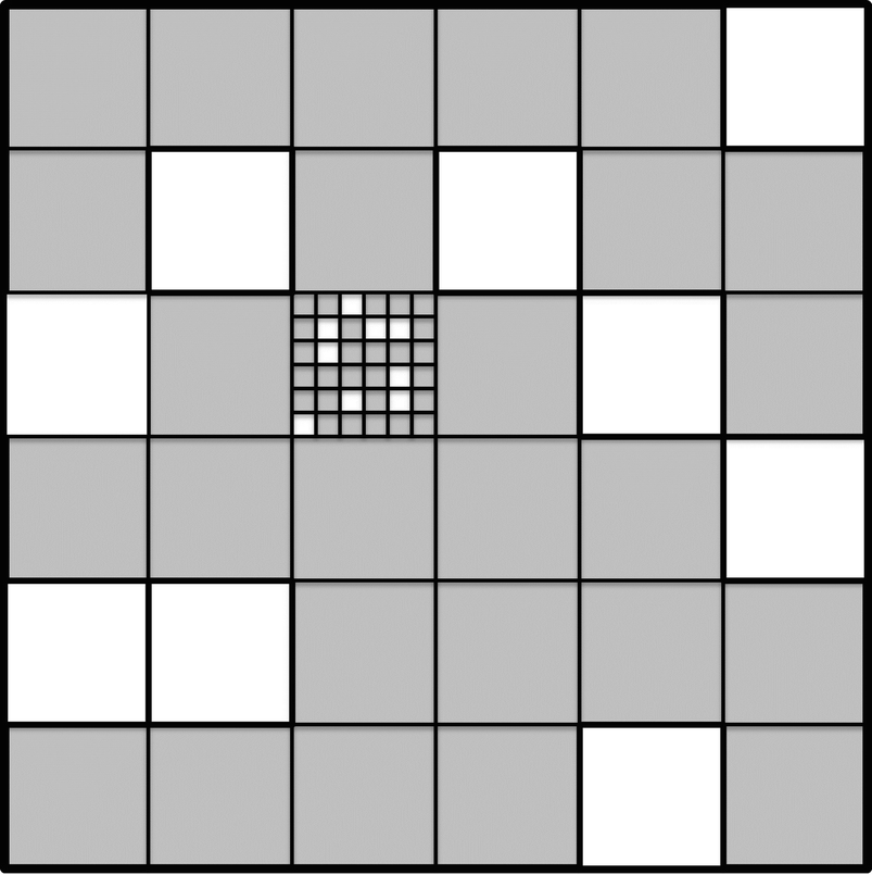
Lacunarity with three hierarchy levels
Three independently chosen probabilities determine whether a region is occupied. Each first-level region is occupied with probability p 1. If a first-level region R 1 is not occupied, then each of the 36 second-level regions within R 1 is declared “not occupied”, and in turn each of the 36 third-level regions within each second-level region in R 1 is also declared “not occupied”. On the other hand, if a first-level region R 1 is occupied, then each second-level region within R 1 is occupied with probability p 2. The same process is used to create the third-level regions. If a second-level region R 2 is not occupied, then each of the 36 third-level regions within R 2 is declared “not occupied”. If a second-level region R 2 is occupied, then each third-level region within R 2 is occupied with probability p 3. Figure 19.6 shows 9 unoccupied first-level regions (shaded white) and 9 unoccupied second-level regions (shaded white) within one of the occupied first-level regions.
Several different strategies for choosing the probabilities were studied. For example, the “same” strategy sets p
1 = p
2 = p
3; this strategy generates statistically self-similar maps. The “bottom” strategy sets p
1 = p
2 = 1 and p
3 = p (for some p ∈ (0, 1)) for each third-level region, so all first-level and second-level regions are occupied; with this strategy the contiguous occupied regions are small, as are the gaps between occupied regions. The “top” strategy sets p
2 = p
3 = 1, so that if a first-level region R
1 is occupied, all second-level and third-level regions within R
1 are occupied; with this strategy the occupied regions are large, as are the gaps between occupied regions. For each strategy,  versus
  was plotted (Figures 8, 9, and 10 in [Plotnick 93]) for r = 2i for i from 0 to 7. The plots for the different strategies form very different curves: e.g., for p = 1∕2 the “top” curve appears concave, the “bottom” curve appears convex, and the “same” curve appears linear (in accordance with the theoretical result that the slope is d
B − E).
was plotted (Figures 8, 9, and 10 in [Plotnick 93]) for r = 2i for i from 0 to 7. The plots for the different strategies form very different curves: e.g., for p = 1∕2 the “top” curve appears concave, the “bottom” curve appears convex, and the “same” curve appears linear (in accordance with the theoretical result that the slope is d
B − E).

 , so N is the total number of points. We have

 . From (19.6) we obtain
The variation of lacunarity with fractal dimension was considered in [Krasowska 04], which mentioned a relation due to Kaye that the local density ρ of a lattice of tiles satisfies ρ ∼ Λd B, where Λ is the average of Λ(s) over a range of box sizes. This relation suggests that there is a negative correlation between Λ and d B. Based on an analysis of polymer surfaces and stains in cancer cells, it was speculated in [Krasowska 04] that the relation ρ ∼ Λd B applies only to surfaces generated by similar mechanisms, which thus show similar types of regularity. When a negative correlation fails to hold, it may be due to the existence of several different surface generation mechanisms.
19.2 Lacunarity Based on an Optimal Covering
A covering of Ω by balls
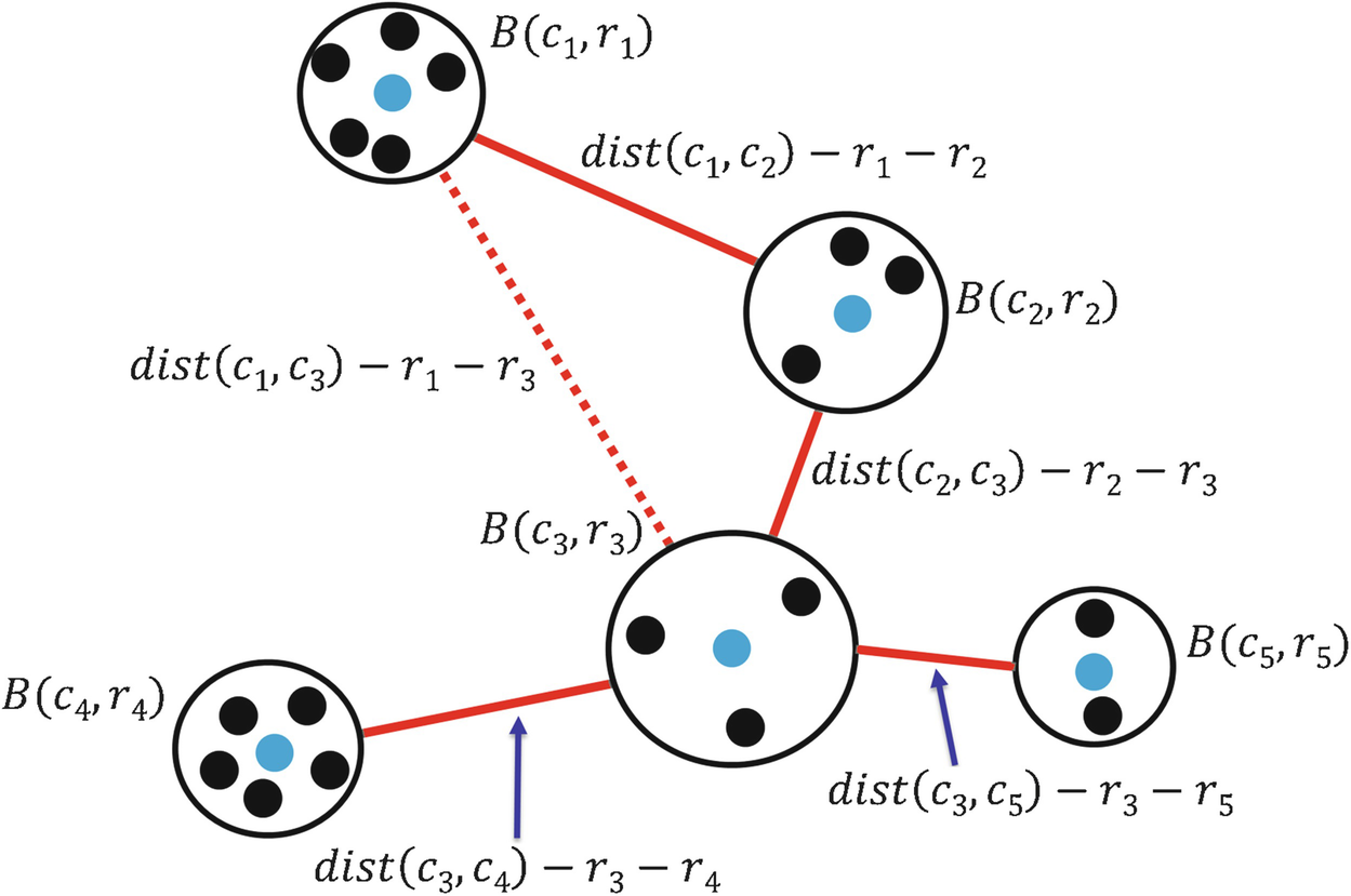
Suppose that, for a given 𝜖, an optimal 𝜖-covering  has been computed; we define “optimal” below. The distance between the ball B(c
i, r
i) and the ball B(c
j, r
j) is c
ij(𝜖) ≡dist(c
i, c
j) − r
i − r
j, where dist(c
i, c
j) is the Euclidean distance between c
i and c
j; having defined c
ij(𝜖), for simplicity we now write c
ij rather than c
ij(𝜖). Since there are J balls in the covering, there are J(J − 1)∕2 inter-ball distances c
ij to compute. Viewing each ball as a “supernode”, the J supernodes and the distances between them form a complete graph.
Compute a minimal spanning tree (MST)
of this graph by any method, e.g., by Prim’s method or Kruskal’s method. Let
has been computed; we define “optimal” below. The distance between the ball B(c
i, r
i) and the ball B(c
j, r
j) is c
ij(𝜖) ≡dist(c
i, c
j) − r
i − r
j, where dist(c
i, c
j) is the Euclidean distance between c
i and c
j; having defined c
ij(𝜖), for simplicity we now write c
ij rather than c
ij(𝜖). Since there are J balls in the covering, there are J(J − 1)∕2 inter-ball distances c
ij to compute. Viewing each ball as a “supernode”, the J supernodes and the distances between them form a complete graph.
Compute a minimal spanning tree (MST)
of this graph by any method, e.g., by Prim’s method or Kruskal’s method. Let  be the set specifying the J − 1 arcs (connecting supernodes) in the MST. This is illustrated in Fig. 19.7. Since there are 5 balls in the cover, then there are 5 supernodes, and 10 arcs interconnecting the supernodes; 5 of these arcs are illustrated (4 using solid red lines, and 1 using a dotted red line). The 4 solid red lines constitute the MST of the complete graph. Thus
  .
.

 , so for Fig. 19.7 we have Λ(𝜖) = c
12 + c
23 + c
34 + c
35.
, so for Fig. 19.7 we have Λ(𝜖) = c
12 + c
23 + c
34 + c
35.Given a set  of points in Ω and given 𝜖 > 0, the major computation burden in the method of [Tolle 03] is computing an optimal 𝜖-covering. Recalling the definition of the Hausdorff dimension and (5.1) in Sect. 5.1, for d > 0 an 𝜖-covering of Ω is optimal if it minimizes
  over all 𝜖-coverings of Ω. Since this definition does not in general lead to a useful algorithm, the approach of [Tolle 03] was to define an optimal covering as a solution to the following optimization problem
  . Let 𝜖 > 0 and the number J of balls in the covering be given. Let
  be the given coordinates of point
  , and let
  be the coordinates (to be determined) of the center of ball j. Define N × J binary variables x
nj, where x
nj = 1 if point n is assigned to ball j, and x
ij = 0 otherwise. We require
be the coordinates (to be determined) of the center of ball j. Define N × J binary variables x
nj, where x
nj = 1 if point n is assigned to ball j, and x
ij = 0 otherwise. We require  for i = 1, 2, …, N; this says that each point in
  must be assigned to exactly one ball. The objective function, to be minimized, is
 ![$$\sum _{j=1}^J \sum _{n=1}^N x_{{{nj}}} [\mathit {dist}( b_{{n}},c_{{j}} )]^2$$](../images/487758_1_En_19_Chapter/487758_1_En_19_Chapter_TeX_IEq31.png) , which is the sum of the squared distance from each point to the center of the ball to which the point was assigned. Optimization problem
, which is the sum of the squared distance from each point to the center of the ball to which the point was assigned. Optimization problem  can be solved using the Picard method [Tolle 03].
After the Picard method has terminated, principal component analysis can be used to compute the inter-cluster distances c
ij.
can be solved using the Picard method [Tolle 03].
After the Picard method has terminated, principal component analysis can be used to compute the inter-cluster distances c
ij.
Exercise 19.1 In Sect. 16.8, we discussed the use by Martinez and Jones [Martinez 90] of a MST to compute d H of the universe. In this section, we discussed the use by Tolle et al. [Tolle 03] of a MST to calculate lacunarity. Contrast these two uses of a MST. □
Exercise 19.2 Although the variables x
nj in the optimization problem  are binary, the Picard method for solving
  treats each x
nj as a continuous variable. Is there a way to approximately solve
treats each x
nj as a continuous variable. Is there a way to approximately solve  which treats each x
nj as binary? Does
which treats each x
nj as binary? Does  become easier to solve if we assume that each ball center c
j is one of the N points? Is that a reasonable assumption? □
become easier to solve if we assume that each ball center c
j is one of the N points? Is that a reasonable assumption? □
19.3 Applications of Lacunarity
Lacunarity has been studied by geologists and environmental scientists (e.g., coexistence through spatial heterogeneity has been shown for both animals and plants [Plotnick 93]), and by chemists and material scientists [Krasowska 04]. We conclude this chapter by describing other applications of lacunarity of a geometric object.
Stone Fences: The aesthetic responses of 68 people to the lacunarity of stone walls, where the lacunarity measures the amount and distribution of gaps between adjacent stones, was studied in [Pilipski 02]. Images were made of stone walls with the same d B but with different lacunarities, which ranged from 0.1 to 4.0. People were shown pairs of images, and asked which one they preferred. There was a clear trend that the preferred images had higher lacunarity, indicating that people prefer images with more texture, and that the inclusion of some very large stones and more horizontal lines will make a stone wall more attractive.
Scar Tissue: In a study to discriminate between scar tissue versus unwounded tissue in mice, [Khorasani 11] computed d B and the lacunarity of mice tissue. Microscope photographs were converted to 512 × 512 pixel images, which were analyzed using the ImageJ package.2 They found that using d B and lacunarity was superior to the rival method of Fourier transform analysis.
The Human Brain: The gliding box method was used by Katsaloulis et al. [Katsaloulis 09] to calculate the lacunarity of neural tracts in the human brain. The human brain consists of white matter and gray matter; white matter “consists of neurons which interconnect various areas of brain together, in the form of bundles. These pathways form the brain structure and are responsible for the various neuro-cognitive aspects. There are about 100 billion neurons within a human brain interconnected in complex manners”. Four images from MRI scans were mapped to an array of 512 × 512 pixels. Using box sizes from 1 to 64 pixels, d B ranged from 1.584 to 1.720. The same range of box sizes was used to compute the lacunarity of each image, where for each box size r the lacunarity Λ(r) was defined by (19.5). It was observed in [Katsaloulis 09] that lacunarity analysis of two images provided a finer or secondary measure (in addition to d B) which may indicate that the neurons originate from different parts of the brain, or may indicate damaged versus healthy tissue. Similarly, [Di Ieva 13] observed that “Lacunarity and d B have been used to show the physiological decline of neuronal and glial structures in the processes of aging, whereby the d B decreases and lacunarity increases in neurons, while the contrary occurs in glial cells, giving rise to a holistic representation of the neuroglial network”. Road Networks: In Sect. 6.5, we described the study of [Sun 12], which computed d B and local dimensions for the road network of Dalian, China. The road network was treated as a geometric object Ω, not as a network, and Ω was superimposed on a 2022 × 1538 grid of cells. For each cell x in the grid, [Sun 12] created a sub-domain Ω(x) of size 128 × 128 cells centered at x; if x is near the boundary, then the sub-domain extended beyond Ω. The sub-domains overlap; the closer the cells x and y are to each other, the greater the overlap. For each x, [Sun 12] restricted attention to Ω(x) and calculated a local box counting dimension d B(x) by the usual procedure of subdividing Ω(x) into boxes of a given size and counting boxes that contain part of the image in Ω(x). Doing this for each cell x in the grid yielded a 2022 × 1538 array of d B(x) values.
The motivation of [Sun 12] for computing these d B(x) values was that the overall dimension d B is useful in comparing cities, but not useful in investigating the heterogeneity of different areas within a single urban road network. The d B(x) were displayed using a color map, with high d B(x) values getting a more red color, and low values getting a more blue color. They also studied how the d B(x) values correlate with the total road length within the sub-domain. However, they did not use the term “lacunarity”, nor did they compute an overall statistic that combines the d B(x).
Air Pollution: Lacunarity was used by Arizabalo et al. [Arizabalo 11] to study air pollution in Mexico. Atmospheric sub-micron particle concentrations were measured for particle sizes ranging from 16 to 764 nm using a Scanning Mobility Particle Sizer. The calculated lacunarity values ranged from 1.095 to 2.294. They found that days of low lacunarity indicated a nucleation particle formation process (with particle diameters of 10–20 nm), medium lacunarity indicated an Aitken process (with particle diameters of 20–100 nm), and high lacunarity indicated an accumulation process (with particle diameters of 100–420 nm). The results showed that lacunarity can be a useful tool for “identifying important changes concerning the particle concentrations (roughness) and size distributions (lagoons), respectively, which occur as a result of dynamic factors such as traffic density, industrial activity, and atmospheric conditions”.
Pre-sliced Cooked Meat: In [Valous 10], lacunarity was computed for slices of meat that were prepared using different percentages of brine solutions and different processing regimes. It was observed in [Valous 10] that, in theory at least, textural information may be lost in the process of converting grayscale images to binary images, so the lacunarity calculated from grayscale images could provide better accuracy for characterization or classification than the lacunarity calculated using binary images. The main objective of this study was to determine the usefulness of different color scales, and compare them to a binary approach. When using a color scale, each pixel in the 256 × 256 image is identified by two coordinates, and has an associated integer “intensity” between 0 and 255. The lacunarity analysis was performed by the FracLac software [Rasband], which determined the average intensity of pixels per gliding box. The study confirmed that the intensity-based lacunarity values are a useful quantitative descriptor of visual texture. However, [Valous 10] also cautioned that discerning and measuring texture is challenging, and while lacunarity is useful, it is not a panacea. Finally, [Valous 10] credited Feagin with the observation that while lacunarity analysis may seem similar to multifractal analysis, “multifractals discern a globally consistent value based upon the singularity of local scaling exponents, whereas lacunarity defines the magnitude of local variations not as they scale
outwards from those localities, but rather between localities”. The extensive reference list in [Valous 10] is an excellent guide to further reading.
Exercise 19.3 The “gliding box” method for computing lacunarity assumed a square matrix. Modify the algorithm to compute the lacunarity for a rectangular matrix. □
 can be partitioned as illustrated in Fig. 19.8, for some square region Ψ of side length L. Let Λ(Ω, s) and Λ(Ψ, s) be the lacunarity of Ω and Ψ, respectively, for box size s. Can we estimate Λ(Ω, s) using Λ(Ψ, s)? □
Ω is partitioned into 16 identical smaller pieces
Exercise 19.5 ⋆ The only network considered in this chapter is a road network [Sun 12] which was studied as a geometric object. Extend the definition of lacunarity to a spatially embedded network, and apply the definition to an example. □
Exercise 19.6 ⋆ Can the definition of lacunarity be extended to a network, not spatially embedded, with arbitrary arc costs? □