There is a fifth dimension, beyond that which is known to man. It is a dimension as vast as space and as timeless as infinity. It is the middle ground between light and shadow, between science and superstition.
Rod Sterling (1924–1975), American screenwriter, playwright, television producer, and narrator, best known for his television series “The Twilight Zone”, which ran from 1959 to 1964
 :
: the Hausdorff dimension, a generalization of the box counting dimension, which has enormous theoretical importance, even though it has been rarely used for computational purposes,
the similarity dimension, which provides a very useful way to calculate the box counting dimension without actually performing box counting, and
This chapter lays the foundation for our study of the similarity dimension of a network (Chap. 13) and our study of the Hausdorff dimension of a network (Chap. 18).the packing dimension, which provides a “dual” way of looking at dimension.
5.1 Hausdorff Dimension
In this section we study the Hausdorff dimension of a bounded set  . Recall first that Definition 4.6 of d
B (Sect. 4.2) allows us to assume that each box in the covering of Ω
has the same size s, where s → 0. Therefore, d
B, which assigns the same “weight” to each non-empty box in the covering of Ω, “may be thought of as indicating the efficiency with which a set may be covered by small sets of equal size” [Falconer 03]. In contrast, the Hausdorff dimension assumes a covering
of Ω by sets of size at most s, where s → 0, and assigns a weight to each set that depends on the size of the set. The Hausdorff dimension was introduced in 1919 by Felix Hausdorff [Hausdorff 19], and historically preceded the box counting dimension.1 Our presentation is based on [Farmer 83, Schleicher 07, Theiler 90]. Let
. Recall first that Definition 4.6 of d
B (Sect. 4.2) allows us to assume that each box in the covering of Ω
has the same size s, where s → 0. Therefore, d
B, which assigns the same “weight” to each non-empty box in the covering of Ω, “may be thought of as indicating the efficiency with which a set may be covered by small sets of equal size” [Falconer 03]. In contrast, the Hausdorff dimension assumes a covering
of Ω by sets of size at most s, where s → 0, and assigns a weight to each set that depends on the size of the set. The Hausdorff dimension was introduced in 1919 by Felix Hausdorff [Hausdorff 19], and historically preceded the box counting dimension.1 Our presentation is based on [Farmer 83, Schleicher 07, Theiler 90]. Let  be a metric space
and let Ω be a bounded subset of
be a metric space
and let Ω be a bounded subset of  .
.
Definition 5.1 For s > 0, an s-covering of Ω is a finite collection of J sets {X
1, X
2, ⋯ , X
J} that cover Ω (i.e.,  ) such that for each j we have diam(X
j) ≤ s. □
) such that for each j we have diam(X
j) ≤ s. □
 be the set of all s-coverings of Ω. For s > 0 and for d ≥ 0, define
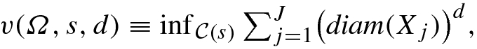
 of Ω. We take the infimum since the goal is to cover Ω with small sets X
j as efficiently as possible.
of Ω. We take the infimum since the goal is to cover Ω with small sets X
j as efficiently as possible. , and
, and  . We have

 and the distance metric dist(⋅, ⋅) is the Euclidean distance and d is a positive integer, v
⋆(Ω, d) is within a constant scaling factor of the Lebesgue measure of Ω.
2 If Ω is countable, then v
⋆(Ω, d) = 0.
and the distance metric dist(⋅, ⋅) is the Euclidean distance and d is a positive integer, v
⋆(Ω, d) is within a constant scaling factor of the Lebesgue measure of Ω.
2 If Ω is countable, then v
⋆(Ω, d) = 0.

 with d
H < 1 is totally disconnected [Falconer 03]. (A set Ω is totally disconnected if for x ∈ Ω, the largest connected component of Ω containing x is x itself.) If
with d
H < 1 is totally disconnected [Falconer 03]. (A set Ω is totally disconnected if for x ∈ Ω, the largest connected component of Ω containing x is x itself.) If  is an open set, then d
H = E. If Ω is countable, then d
H = 0. A function
is an open set, then d
H = E. If Ω is countable, then d
H = 0. A function  is bi-Lipschitz
if for some positive numbers α and β and for each x, y ∈ Ω, we have
is bi-Lipschitz
if for some positive numbers α and β and for each x, y ∈ Ω, we have 
 ; that is, the Hausdorff dimension of Ω is unchanged by a bi-Lipschitz transformation. In particular, the Hausdorff dimension of a set is unchanged by rotation or translation.
 is a measurable subset of Ω, then we can similarly form
  , and in particular, choosing d = d
H(Ω) we can form
, and in particular, choosing d = d
H(Ω) we can form  . The function
For ordinary geometric objects, the Hausdorff and box counting dimensions are equal: d
H = d
B. However, in general we only have d
H ≤ d
B, and there are many examples where this inequality is strict [Falconer 03]. To prove this inequality, we will use Definition 4.6 of d
B with B(s) defined as the minimal number of boxes of size s needed to cover Ω. Recall that the lower box counting dimension  is defined by (4.2) and if d
B exists then
is defined by (4.2) and if d
B exists then  .
.
Theorem 5.1  .
.
Proof [
Falconer 03] Suppose Ω can be covered by B(s) boxes of diameter s.
By (5.1), for d ≥ 0 we have v(Ω, s, d) ≤ B(s)s
d. Since v
⋆(Ω, d) = ∞ for d < d
H, then for d < d
H we have v
⋆(Ω, d) =lims→0v(Ω, s, d) > 1. Hence for d < d
H and s sufficiently small, B(s)s
d ≥ v(Ω, s, d) > 1, which implies  . Rewriting this as
  , it follows that
  . Since this holds for d < d
H, then
. Since this holds for d < d
H, then  . □
. □
Example 5.1 Let Ω be the unit square in  . Cover Ω with J
2 squares, each with side length s = 1∕J. Using the L
1 metric (i.e., ||x|| =maxi=1,2 |x
i|), the diameter of each box is 1∕J. We have
. Cover Ω with J
2 squares, each with side length s = 1∕J. Using the L
1 metric (i.e., ||x|| =maxi=1,2 |x
i|), the diameter of each box is 1∕J. We have  , and limJ→∞J
2−d = ∞ for d < 2 and limJ→∞J
2−d = 0 for d > 2. Since v
⋆(Ω, d) = 0 for d > 2, then by Definition 5.2 we have d
H ≤ 2. □
, and limJ→∞J
2−d = ∞ for d < 2 and limJ→∞J
2−d = 0 for d > 2. Since v
⋆(Ω, d) = 0 for d > 2, then by Definition 5.2 we have d
H ≤ 2. □


 . Thus
  . However, this argument provides no information about a lower bound for d
H. For example, if the self-similar set Ω is countable, then its Hausdorff dimension is 0. The above examples illustrate that it is easier to obtain an upper bound on d
H than a lower bound. Obtaining a lower bound on d
H requires estimating all possible coverings of Ω. Interestingly, there is a way to compute a lower bound on the box counting dimension of a network (Sect. 8.8).
. However, this argument provides no information about a lower bound for d
H. For example, if the self-similar set Ω is countable, then its Hausdorff dimension is 0. The above examples illustrate that it is easier to obtain an upper bound on d
H than a lower bound. Obtaining a lower bound on d
H requires estimating all possible coverings of Ω. Interestingly, there is a way to compute a lower bound on the box counting dimension of a network (Sect. 8.8). . Given that the volume V
E(r) of a ball with radius r in E-dimensional Euclidean space is3
. Given that the volume V
E(r) of a ball with radius r in E-dimensional Euclidean space is3 


In [Bez 11] it was observed that d H is a local, not global, property of Ω, since it is defined in terms of a limit as s → 0. That is, even though d H is defined in terms of a cover of Ω by sets of diameter at most s, since s → 0 then d H is still a local property of Ω. The term “roughness” was used in [Bez 11] to denote that characteristic of Ω which is quantified by d H. Also, [Bez 11] cautioned that the fact that, while fractal sets are popular mainly for their self-similar properties, computing a fractal dimension of Ω does not imply that Ω is self-similar. In applications of fractal analysis to ecology, there are many systems which exhibit roughness but not self-similarity, but the systems of strong interest exhibit either self-similarity or they exhibit self-similarity and roughness. However, assessing self-similarity is a challenging if not impossible task without an a priori reason to believe that the data comes from a model exhibiting self-similarity (e.g. fractionary Brownian processes). The notion that the ability to compute a fractal dimension does not automatically imply self-similarity holds not only for a geometric object, but also for a network (Chaps. 18 and 21).
In [Jelinek 06] it was observed that although the Hausdorff dimension is not usable in practice, it is important to be aware of the shortcomings of methods, such as box counting, for estimating the Hausdorff dimension. In studying quantum gravity, [Ambjorn 92] wrote that the Hausdorff dimension is a very rough measure of geometrical properties, which may not provide much information about the geometry.5 The distinction between d H and d B is somewhat academic, since very few experimenters are concerned with the Hausdorff dimension. Similarly, [Badii 85] observed that, even though there are examples where d H ≠ d B, “it is still not clear whether there is any relevant difference in physical systems.”6 In practice the Hausdorff dimension of a geometric object has been rarely used, while the box counting dimension has been widely used, since it is rather easy to compute.The concept of “dimension” is elusive and very complex, and is far from exhausted by [these simple considerations]. Different definitions frequently yield different results, and the field abounds in paradoxes. However, the Hausdorff-Besicovitch dimension and the capacity dimension, when computed for random self-similar figures, have so far yielded the same value as the similarity dimension.4
 . To be called a dimension function, dim(⋅) should satisfy the following for any subsets
  and
and  of Ω:
of Ω: Falconer observed that all definitions of dimension are monotonic, most are stable, but some common definitions do not exhibit countable stability and may have countable sets of positive dimension. The open sets and smooth manifolds conditions ensure that the classical definition of dimension is preserved. The monotonicity condition was used in [Rosenberg 16b] to study the correlation dimension of a rectilinear grid network (Sect. 11.4). All the above properties are satisfied by the Hausdorff dimension d H. As to whether these properties are satisfied by the box counting dimension, we have [Falconer 03] (i) the lower and upper box counting dimensions are monotonic; (ii) the upper box counting dimension is finitely stable, i.e.,monotonicity: If
then
.
stability: If
and
are subsets then
.
countable stability: If
is an infinite collection of subsets then
.
countable sets: If
is finite or countably infinite then
.
open sets: If
is an open subset of
then
.
smooth manifolds: If
is a smooth (i.e., continuously differentiable) E-dimensional manifold (curve, surface, etc.) then
.
 ; (iii) the box counting dimension of a smooth E-dimensional manifold in
  is E; also, the lower and upper box counting dimensions are bi-Lipschitz invariant.
5.2 Similarity Dimension
The next definition of dimension we study is the similarity dimension [Mandelbrot 83b], applicable to an object which looks the same when examined at any scale. We have already encountered, in the beginning of Chap. 3, the idea of self-similarity when we considered the Cantor set. For self-similar fractals, the similarity dimension is a way to compute a fractal dimension without computing the slope of the  versus
  curve.
 .
.
Self-similarity with K = 8 and α = 1∕4
 uses the same contraction factor α, and the functions f
k differ only in the amount of rotation or translation they apply to a point in
uses the same contraction factor α, and the functions f
k differ only in the amount of rotation or translation they apply to a point in  (recall that a point in
  is a non-empty compact subset of a metric space
  ).
The IFS theory guarantees the existence of an attractor Ω of the IFS.
The heuristic argument (not a formal proof) leading to the similarity dimension is as follows. Let B(s) be the minimal number of boxes of size s needed to cover Ω.
).
The IFS theory guarantees the existence of an attractor Ω of the IFS.
The heuristic argument (not a formal proof) leading to the similarity dimension is as follows. Let B(s) be the minimal number of boxes of size s needed to cover Ω.
Three generations of a self-similar fractal


 . If we cover Ω with boxes of size s∕α, the minimal number of boxes required is
  .
.
 , and this equality can be written as

Example 5.3 Consider the Sierpiński triangle of Fig. 3.3. In each iteration we shrink the object by the factor α = 1∕2, and take K = 3 copies of the reduced figure. From (5.8) we have  . □
. □
Example 5.4 Consider the Sierpiński carpet of Fig. 4.10. In each iteration we shrink the object by the factor α = 1∕3, and take K = 8 copies of the reduced figure. Thus  . □
. □
Example 5.5 Consider the Cantor set of Fig. 3.2. In each iteration we shrink the object by the factor α = 1∕3, and take K = 2 copies of the reduced figure. Thus  . □
. □
Example 5.6 We can generalize the Cantor set construction, as described in [Schleicher 07].
We start with the unit interval, and rather than remove the middle third, we remove a segment of length 1 − 2x from the middle, where x ∈ (0, 1∕2). This leaves two segments, each of length x. In subsequent iterations, we remove from each segment an interval in the middle with the same fraction of length. Let C
t be the pre-fractal
set obtained after t iterations of this construction. From (5.8) we have  . Since d
S → 1 as x → 1∕2 and d
S → 0 as x → 0, the similarity dimension can assume any value in the open interval (0, 1). □
. Since d
S → 1 as x → 1∕2 and d
S → 0 as x → 0, the similarity dimension can assume any value in the open interval (0, 1). □
Example 5.7 Consider the Cantor dust of Fig. 4.12.
This figure can be described as the Cartesian product  of the Cantor set
  with itself. We construct Cantor dust by taking, in generation t, the Cartesian product
  , where
  is defined in Example 5.6 above. The similarity dimension of the generalized Cantor dust is
  , where x ∈ (0, 1). Since d
S → 2 as x → 1∕2 and d
S → 0 as x → 0, the similarity dimension can assume any value in the open interval (0, 2). □
, where x ∈ (0, 1). Since d
S → 2 as x → 1∕2 and d
S → 0 as x → 0, the similarity dimension can assume any value in the open interval (0, 2). □

 , where x ∈ (0, 1). Since d
S → E as x → 1∕2 and d
S → 0 as x → 0, the similarity dimension can assume any value in the open interval (0, E). This example demonstrates why defining a fractal to be a set with a non-integer dimension may not be a particularly good definition. It seems unreasonable to consider E-dimensional generalized Cantor dust to be a fractal only if
, where x ∈ (0, 1). Since d
S → E as x → 1∕2 and d
S → 0 as x → 0, the similarity dimension can assume any value in the open interval (0, E). This example demonstrates why defining a fractal to be a set with a non-integer dimension may not be a particularly good definition. It seems unreasonable to consider E-dimensional generalized Cantor dust to be a fractal only if  is not an integer. □
 . Considering levels 0 and 2, the ratio of the microfibril diameter to the α-helix diameter is 8.619, and there are 33 α-helix macromolecules per microfibril. Thus the next similarity dimension is
  . Finally, considering levels 0 and 3, the ratio of the macrofibril diameter to the α-helix diameter is 17.842, and there are 99 α-helix macromolecules per microfibril. Thus that similarity dimension is
  . The authors noted that d
0↔2 and d
0↔3 are close to the “golden mean” value
. The authors noted that d
0↔2 and d
0↔3 are close to the “golden mean” value  , and conjectured that this is another example of the significant role of the golden mean in natural phenomena. □
The above discussion of self-similar fractals assumed that each of the K instances of Ω is reduced by the same scaling factor α. We can generalize this to the case where Ω is decomposed into K non-identical parts, and the scaling factor α
k is applied to the k-th part, where 0 < α
k < 1 for 1 ≤ k ≤ K. Some or all of the α
k values may be equal; the self-similar case is the special case where all the α
k values are equal. The construction for the general case corresponds to an IFS
for which each of the K functions  does not necessarily use the same contraction factor, but aside from the possibly different contraction factors, the functions f
k differ only in the amount of rotation or translation they apply to a point in
does not necessarily use the same contraction factor, but aside from the possibly different contraction factors, the functions f
k differ only in the amount of rotation or translation they apply to a point in  . That is, up to a constant scaling factor, the f
k differ only in the amount of rotation or translation.
. That is, up to a constant scaling factor, the f
k differ only in the amount of rotation or translation.

 , yielding
  , which is precisely (5.8).


Example 5.10 Suppose the Cantor set construction of Fig. 3.2 is modified so that we take the first 1∕4 and the last 1∕3 of each interval to generate the next generation intervals. Starting in generation 0 with [0, 1], the generation-1 intervals are ![$$[0,\frac {1}{4}]$$](../images/487758_1_En_5_Chapter/487758_1_En_5_Chapter_TeX_IEq82.png) and
and ![$$[\frac {2}{3}, 1]$$](../images/487758_1_En_5_Chapter/487758_1_En_5_Chapter_TeX_IEq83.png) . The four generation-2 intervals are (i)
. The four generation-2 intervals are (i) ![$$[0,(\frac {1}{4})(\frac {1}{4})]$$](../images/487758_1_En_5_Chapter/487758_1_En_5_Chapter_TeX_IEq84.png) , (ii)
, (ii) ![$$[\frac {1}{4}-(\frac {1}{3})(\frac {1}{4}), \frac {1}{4}]$$](../images/487758_1_En_5_Chapter/487758_1_En_5_Chapter_TeX_IEq85.png) , (iii)
, (iii) ![$$[\frac {2}{3}, \frac {2}{3} + (\frac {1}{4})(\frac {1}{3})]$$](../images/487758_1_En_5_Chapter/487758_1_En_5_Chapter_TeX_IEq86.png) , and (iv)
, and (iv) ![$$[1-(\frac {1}{3})(\frac {1}{3}) ,1]$$](../images/487758_1_En_5_Chapter/487758_1_En_5_Chapter_TeX_IEq87.png) . From (5.12), with K = 2, α
1 = 1∕4, and α
2 = 1∕3, we obtain
. From (5.12), with K = 2, α
1 = 1∕4, and α
2 = 1∕3, we obtain  , which yields d
S ≈ 0.560; this is smaller than the value
, which yields d
S ≈ 0.560; this is smaller than the value  obtained for K = 2 and α
1 = α
2 = 1∕3. □
obtained for K = 2 and α
1 = α
2 = 1∕3. □
In general, the similarity dimension of Ω is not equal to the Hausdorff dimension of Ω. However, if the following Open Set Condition holds, then the two dimensions are equal [Glass 11].
 be a metric space,
and let Ω be a non-empty compact subset of
be a metric space,
and let Ω be a non-empty compact subset of  . Suppose for the IFS
  with contraction factors
  we have
  . Then the IFS
  satisfies the Open Set Condition if there exists a non-empty open
set
satisfies the Open Set Condition if there exists a non-empty open
set  such that
In practice, the Open Set Condition can be easy to verify.
Example 5.11 The Cantor Set can be generated by an IFS using two similarities defined on  . Let
. Let  and
and  . The associated ratio list is
  . The invariant set of this IFS is the Cantor set. The similarity dimension of the Cantor set satisfies
  , so
, so  . To verify the Open Set Condition, choose U = (0, 1). Then
  and
and  , so f
1(U) ∩ f
2(U) = ∅ and f
1(U) ∪ f
2(U) ⊂ U. Thus the Open Set Condition holds. □
, so f
1(U) ∩ f
2(U) = ∅ and f
1(U) ∪ f
2(U) ⊂ U. Thus the Open Set Condition holds. □
 . Treating
  as a column vector (i.e., a 2 × 1 matrix),
the IFS generating this fractal uses the three similarities
as a column vector (i.e., a 2 × 1 matrix),
the IFS generating this fractal uses the three similarities ![$$\displaystyle \begin{aligned} {f_{{\, 1}}}(x) = Mx, \;\;\;\; {f_{{\, 2}}}(x) = Mx+\left( \begin{array}{c} \frac{1}{2} \\ 0 \end{array} \right), \;\;\;\; {f_{{\, 3}}}(x) = Mx+\left( \begin{array}{c} \frac{1}{4} \\[0.5em] \frac{\sqrt{3}}{4} \end{array} \right) , \end{aligned}$$](../images/487758_1_En_5_Chapter/487758_1_En_5_Chapter_TeX_Equn.png)

 , and (1, 0). As illustrated in Fig. 5.4, f
1(U) is the open triangle with corner points (0, 0),
, and (1, 0). As illustrated in Fig. 5.4, f
1(U) is the open triangle with corner points (0, 0),  , and
, and  ; f
2(U) is the open triangle with corner points
; f
2(U) is the open triangle with corner points  ,
,  , and (1, 0); and f
3(U) is the open triangle with corner points
, and (1, 0); and f
3(U) is the open triangle with corner points  ,
,  , and
, and  . Thus f
i(U) ∩ f
j(U) = ∅ for i ≠ j and f
1(U) ∪ f
2(U) ∪ f
3(U) ⊂ U, so the condition holds. □
. Thus f
i(U) ∩ f
j(U) = ∅ for i ≠ j and f
1(U) ∪ f
2(U) ∪ f
3(U) ⊂ U, so the condition holds. □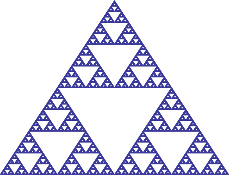
Sierpiński triangle
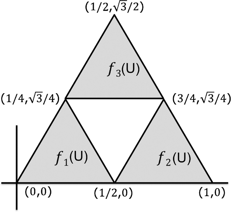
The Open Set Condition for the Sierpiński gasket
Example 5.13 An example of an IFS and a set U for which (5.13) does not hold was given by McClure.7 Pick  . Define f
1(x) = rx and f
2(x) = rx + (1 − r). Choosing U = (0, 1), we have f
1(U) = (0, r) and f
2(U) = (1 − r, 1). Since
. Define f
1(x) = rx and f
2(x) = rx + (1 − r). Choosing U = (0, 1), we have f
1(U) = (0, r) and f
2(U) = (1 − r, 1). Since  , the union of (0, r) and (1 − r, 1) is (0, 1) and the intersection of (0, r) and (1 − r, 1) is the non-empty set (1 − r, r), so (5.13) does not hold for this U. Note that blindly calculating the similarity dimension with K = 2, we obtain
  , and the box counting dimension of [0, 1] is 1. □
Exercise 5.1 Construct an IFS and a set U in  for which (5.13) does not hold. □
5.3 Fractal Trees and Tilings from an IFS
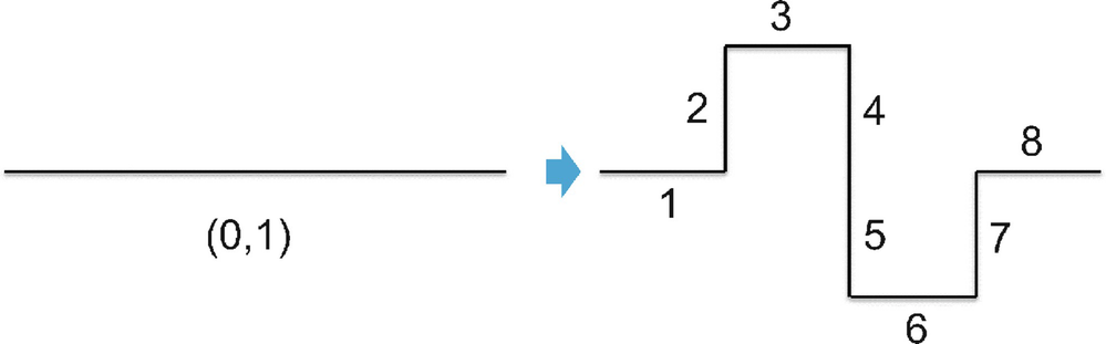
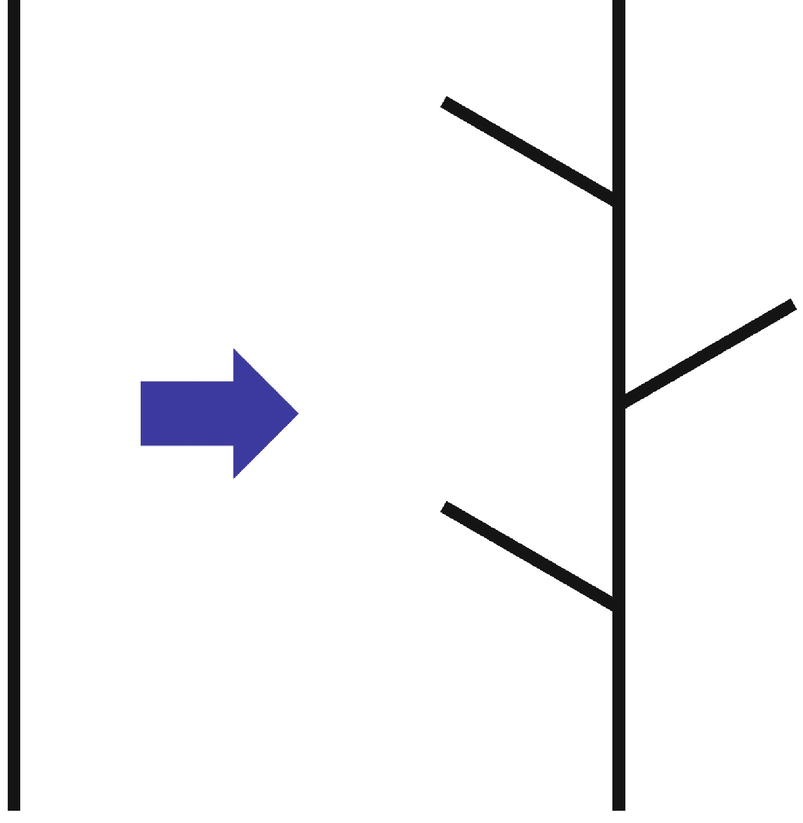
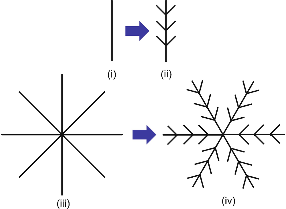
Mandelbrot [Mandelbrot 83b] first hypothesized that rivers are fractal, and introduced fractal objects similar to river networks. With the goal of unifying different approaches to the computation of the fractal dimension of a river, [Claps 96] described a tree generation method using an IFS (Sect. 3.3), in which an initiator (usually a unit-length line segment) is replaced by a generator (which is a tree-like structure of M arcs, each of length L). After a replacement, each segment of the generator becomes an initiator and is replaced by the generator; this process continues indefinitely.
 . Figure 5.6, from [Claps 96], illustrates a topology generator. In this figure, each of the three branches has length one-fourth the length of the initiator on the left. Since the tree on the right has seven equal length segments, then the dimension of this fractal generated from this topology generator is
  . Let
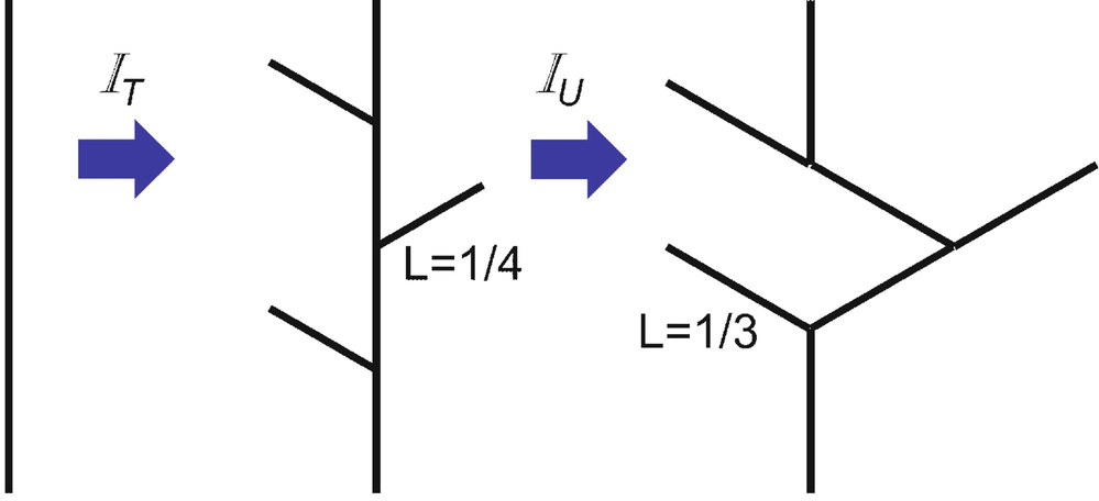
. Let  denote the above sinuosity generator, and let
  denote the above topology generator. Now define
  , which means we first apply
  and then apply
  . As applied to the straight line initiator, the result of applying
  is illustrated by Fig. 5.7.
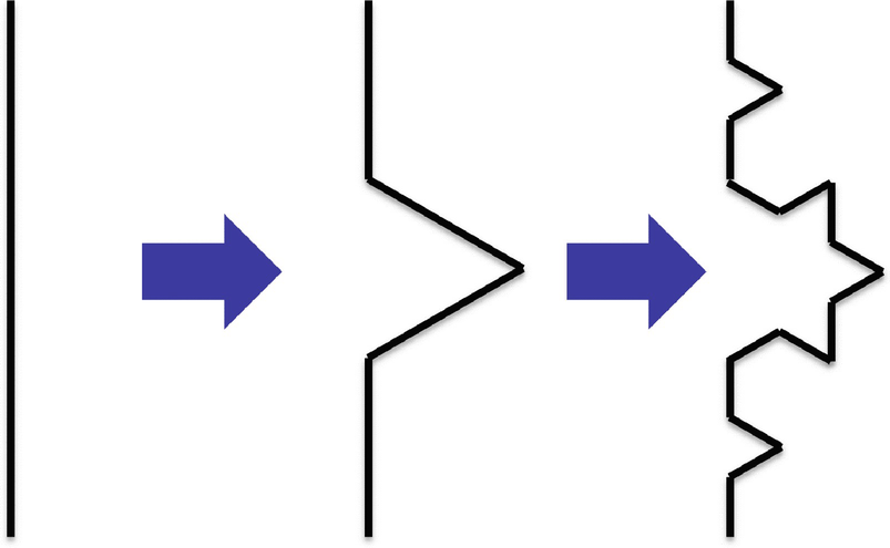
Sinuosity generator  based on the Koch fractal
Topology generator 
 applied to a straight line initiator
 is to make the length of each of the seven line segments created by
  equal to 1/3. Since in this figure there are seven segments, each of which is one-third the length of the initiator, then this fractal has similarity dimension
  . The similarity dimension of
  is equal to the product of the similarity dimensions of
  and
and  ; that is,
 requires that the initial tree have equal arc lengths, and all angles between arcs be a multiple of π∕2 radians (i.e., all angles must be right angles).
Although the above analysis was presented in [Claps 96] without reference to nodes and arcs, it could have been presented in a network context, by defining an arc to be a segment and a node to be the point where two segments intersect. Suppose M
U = 1∕L
T, so the similarity dimension of  is equal to the product of the similarity dimensions of
  and
and  . We express this relationship as
  . The scaling factor of the IFS is α = 1∕L
T, and
. The scaling factor of the IFS is α = 1∕L
T, and  is the fractal dimension of the fractal tree generated by this IFS. For t > 1, the tree network
  constructed in generation t by this IFS is a weighted network, since each arc length is less than 1.
 . □
. □
IFS for goose down
Exercise 5.2 Describe the above goose down construction by an IFS, explicitly specifying the similarities and contraction factors. □
A Penrose tiling
[Austin 05] of  can be viewed as network that spans all of
  . These visually stunning tilings can be described using an IFS, as described in [Ramachandrarao 00], which considered a particular tiling based on a rhombus, and observed that quasi crystals have been shown to pack in this manner.8 An interesting feature of this tiling is that the number of node and arcs can be represented using the Fibonacci numbers. Letting N(s) be the number of arcs of length s in the tiling, they defined the fractal dimension of the tiling to be
  and called this dimension the “Hausdorff dimension” of the tiling. Since the distance between two atoms
in a quasi crystal cannot be zero, when considering the Penrose packing from a crystallographic point of view, a limit has to be placed on the number of iterations of the IFS; for this tiling, the atomic spacing limit was reached in 39 iterations. In [Ramachandrarao 00], a fractal dimension of 1.974 was calculated for the tiling obtained after 39 iterations, and it was observed that the fractal dimension approaches 2 as the number of iterations tends to infinity, implying a “non-fractal space filling structure.” Thus [Ramachandrarao 00] implicitly used the definition that a fractal is an object with a non-integer dimension.
and called this dimension the “Hausdorff dimension” of the tiling. Since the distance between two atoms
in a quasi crystal cannot be zero, when considering the Penrose packing from a crystallographic point of view, a limit has to be placed on the number of iterations of the IFS; for this tiling, the atomic spacing limit was reached in 39 iterations. In [Ramachandrarao 00], a fractal dimension of 1.974 was calculated for the tiling obtained after 39 iterations, and it was observed that the fractal dimension approaches 2 as the number of iterations tends to infinity, implying a “non-fractal space filling structure.” Thus [Ramachandrarao 00] implicitly used the definition that a fractal is an object with a non-integer dimension.
Exercise 5.3
 Pick a Penrose tiling, and explicitly specify the IFS needed to generate the tiling. □
5.4 Packing Dimension
 . A “dual” approach to defining the dimension of Ω is to pack Ω with the largest number of pairwise disjoint balls whose centers lie in Ω, and where the radius of each ball does not exceed r. Our presentation of the packing dimension is based on [Edgar 08]. By a ball we mean a set
 and radius r.
Definition 5.5 Let  be a finite collection of B
P(r) pairwise disjoint balls such that for each ball we have x
j ∈ Ω and r
j ≤ r.9 We do not require that X(x
j, r
j) ⊂ Ω. We call such a collection an r-packing of Ω. Let
be a finite collection of B
P(r) pairwise disjoint balls such that for each ball we have x
j ∈ Ω and r
j ≤ r.9 We do not require that X(x
j, r
j) ⊂ Ω. We call such a collection an r-packing of Ω. Let  denote the set of all r-packings of Ω. □
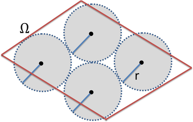
Packing the diamond region with four balls
![$$\displaystyle \begin{aligned} \begin{array}{rcl} \sum_{j=1}^{B_{{P}}(r)} \left[ \mathit{diam} \big( X(x_{{j}},r_{{j}}) \big) \right]^d . {} \end{array} \end{aligned} $$](../images/487758_1_En_5_Chapter/487758_1_En_5_Chapter_TeX_Equ16.png)
 . By choosing long skinny ovals, for d > 0 we can make the sum (5.14) arbitrarily large. While packing with hypercubes works well for a set
  , to have a definition that works in a general metric space,
we pack with balls. Since a subset of a metric space may contain no balls at all, we drop the requirement that each ball in the packing be contained in Ω. However, to ensure that the packing provides a measure of Ω, we require the center of each ball in the packing to lie in Ω. The balls in the packing are closed balls, but open balls could also be used.
, to have a definition that works in a general metric space,
we pack with balls. Since a subset of a metric space may contain no balls at all, we drop the requirement that each ball in the packing be contained in Ω. However, to ensure that the packing provides a measure of Ω, we require the center of each ball in the packing to lie in Ω. The balls in the packing are closed balls, but open balls could also be used.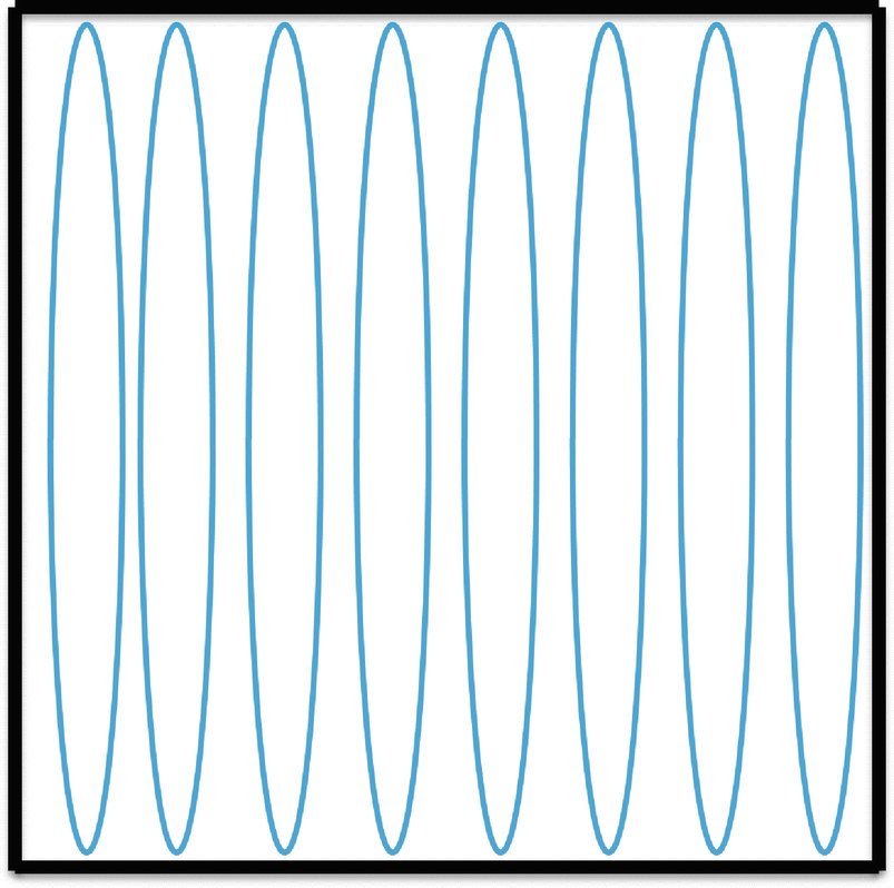
Packing a square with long skinny rectangles
 , since the diameter
of a ball of radius r is 2r. However, there are metric spaces for which this is not true. Thus, rather than maximizing (5.14), we maximize, over all r-packings, the sum
, since the diameter
of a ball of radius r is 2r. However, there are metric spaces for which this is not true. Thus, rather than maximizing (5.14), we maximize, over all r-packings, the sum 

 denotes the supremum over all r-packings of Ω. As r decreases to 0, the set
  shrinks, so the supremum in (5.15) decreases. Define


 of Ω by closed sets, and where f(C, d) is defined by (5.16). If we restrict Ω to be a measurable set, then f
⋆(Ω, d) is a measure, called the d-dimensional packing measure. Finally, if Ω is a Borel set,10 there is a critical value d
P ∈ [0, ∞] such that
of Ω by closed sets, and where f(C, d) is defined by (5.16). If we restrict Ω to be a measurable set, then f
⋆(Ω, d) is a measure, called the d-dimensional packing measure. Finally, if Ω is a Borel set,10 there is a critical value d
P ∈ [0, ∞] such that 
 . Also, if
  then the one-dimensional packing measure coincides with the Lebesgue measure [Edgar 08].
Since d
H considers the smallest number of sets that can cover Ω, and d
P considers the largest number of sets that can be packed in Ω, one might expect a duality theory to hold, and it does. It can be shown [Edgar 08] that if Ω is a Borel subset of a metric space, then d
H ≤ d
P. This leads to another suggested definition [Edgar 08] of the term “fractal”: the set  is a fractal if d
H = d
P; it was mentioned in [Cawley 92] that this definition is due to S.J. Taylor. Under this definition, the real line
is a fractal if d
H = d
P; it was mentioned in [Cawley 92] that this definition is due to S.J. Taylor. Under this definition, the real line  is a fractal, so this definition is not particularly enlightening.
 of Ω is said to be r-separated if dist(x, y) ≥ r for all distinct points
  . In Fig. 5.9, the centers of the four circles are (2r)-separated. Let B
P(r) be the maximal cardinality of an r-separated subset of Ω. Then d
P satisfies
. In Fig. 5.9, the centers of the four circles are (2r)-separated. Let B
P(r) be the maximal cardinality of an r-separated subset of Ω. Then d
P satisfies 
5.5 When Is an Object Fractal?
We have already discussed some suggested definitions of “fractal.” In this section we present, in chronological order, additional commentary on the definition of a “fractal.”
But how should a fractal set be defined? In 1977, various pressures had made me advance the “tentative definition”, that a fractal is “a set whose Hausdorff-Besicovitch dimension strictly exceeds its topological dimension”. But I like this definition less and less, and take it less and less seriously. One reason resides in the increasing importance of the “borderline fractals”, for example of sets which have the topologically “normal” value for the Hausdorff dimension, but have anomalous values for some other metric dimension. I feel - the feeling is not new, as it had already led me to abstain from defining “fractal” in my first book of 1975 - that the notion of fractal is more basic than any particular notion of dimension. A more basic reason for not defining fractals resides in the broadly-held feeling that the key factor to a set’s being fractal is invariance under some class of transforms, but no one has yet pinned this invariance satisfactorily. Anyhow, I feel that leaving the fractal geometry of nature without dogmatic definition cannot conceivably hinder its further development.
Mandelbrot [Mandelbrot 75] himself, the father of the concept, did not provide the scientific community with a clear and unique definition of fractal in his founding literature which was written in French. This was indeed deliberate as stated by Mandelbrot [Mandelbrot 77] himself in the augmented English version published 2 years later: “the French version deliberately avoided advancing a definition” (p. 294). The mathematical definition finally coined in 1977 stated that “an object is said to be fractal if its Hausdorff-Besicovitch dimension d H is greater than its topological dimension d T”.
Theiler divided fractals into either solid objects or strange attractors; [Theiler 90] predated the application of fractal methods to networks, with the significant exception of [Nowotny 88], studied in Chap. 12. Examples of solid object fractals are coastlines, electrochemical deposits, porous rocks, spleenwort ferns, and mammalian brain folds.12 Strange attractors, on the other hand, are conceptual fractal objects that exist in the state space of chaotic dynamical systems (Chap. 9).Fractals are crinkly objects that defy conventional measures, such as length and area, and are most often characterized by their fractal dimension.
 ). To generate the Lévy curve using the basic step, start with (ii) and replace each of the three lines by an angled pair of lines, yielding (iii). After 12 iterations, we obtain Fig. 5.12. 13 The similarity dimension is
  , so this curve is “space-filling” in
  , and d
B = d
S. It follows from a theorem in [Falconer 89] that d
H = d
B. In [Lauwerier 91], it was deemed “a pity” that, under Mandelbrot’s 1977 definition, the Lévy curve does not get to be called a fractal. Lauwerier continued with “Let it be said again: the essential property of a fractal is indefinitely continuing self-similarity. Fractal dimension is just a by-product.” In a later edition of The Fractal Geometry of Nature, Mandelbrot regretted having proposed a strict definition of fractals [Briggs 92]. In 1989, [Mandelbrot 89] observed that fractal geometry “… is not a branch of mathematics like, for example, the theory of measure and integration. It fails to have a clean definition and unified tools, and it fails to be more or less self contained.”
, and d
B = d
S. It follows from a theorem in [Falconer 89] that d
H = d
B. In [Lauwerier 91], it was deemed “a pity” that, under Mandelbrot’s 1977 definition, the Lévy curve does not get to be called a fractal. Lauwerier continued with “Let it be said again: the essential property of a fractal is indefinitely continuing self-similarity. Fractal dimension is just a by-product.” In a later edition of The Fractal Geometry of Nature, Mandelbrot regretted having proposed a strict definition of fractals [Briggs 92]. In 1989, [Mandelbrot 89] observed that fractal geometry “… is not a branch of mathematics like, for example, the theory of measure and integration. It fails to have a clean definition and unified tools, and it fails to be more or less self contained.”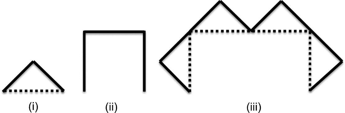
Constructing the Lévy curve
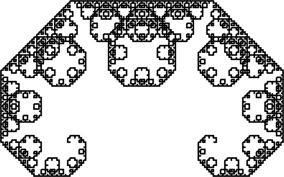
The Lévy curve after 12 iterations
Making no reference to the concept of dimension, fractals were defined in [Shenker 94] “… as objects having infinitely many details within a finite volume of the embedding space. Consequently, fractals have details on arbitrarily small scales, revealed as they are magnified or approached.” Shenker stated that this definition is equivalent to Mandelbrot’s definition of a fractal as an object having a fractal dimension greater than its topological dimension. As we will discuss in Sect. 20.4, Shenker argued that fractal geometry does not model the natural world; this opinion is most definitely not a common view.

Pythagoras tree after 15 iterations
characteristic is a non-integer dimension. The conclusion in [Jelinek 98] was that self-similarity or the fractal dimension are not “absolute indicators” of whether an object is fractal.
It was also observed in [Jelinek 98] that the ability to calculate a fractal dimension of a biological image does not necessarily imply that the image is fractal. Natural objects are not self-similar, but rather are scale invariant over a range, due to slight differences in detail between iteration (i.e., hierarchy) levels. The limited resolution of any computer screen necessarily implies that any biological image studied is pre-fractal. Also, the screen resolution impacts the border roughness of an object and thus causes the computed fractal dimension to deviate from the true dimension. Thus the computed dimension is not very precise or accurate, and is not significant beyond the second decimal place. However, the computed dimension is useful for object classification.
We are cautioned in [Halley 04] that, because fractals are fashionable, there is a natural tendency to see fractals everywhere. Moreover, it was observed in [Halley 04] that the question of deciding whether or not an object is fractal has received little attention. For example, any pattern, whether fractal or not, when analyzed by box counting and linear regression may yield an excellent linear fit, and logarithmic axes tend to obscure deviations from a power-law relationship that might be quite evident using linear scales. In [Halley 04], some sampling and Monte Carlo approaches were proposed to address this question, and it was noted that higher-order Rényi dimensions (Chap. 16) and maximum likelihood schemes can be applied to estimate dimension, but that these methods often utilize knowledge of the process generating the pattern, and hence cannot be used in an “off the shelf” manner as box counting methods can. Indeed, [Mandelbrot 97] observed that fractal geometry “cannot be automated” like analysis of variance or regression, and instead one must always “look at the picture.”