A mind once stretched by a new idea never regains its original dimension.
Oliver Wendell Holmes, Jr. (1841–1935), American, U.S. Supreme Court justice from 1902 to 1932.
A fractal is often defined as a set whose fractal dimension differs from its topological dimension. To make sense of this definition, we start by defining the topological dimension of a set. After that, the remainder of this chapter is devoted to the box counting dimension, which is the first fractal dimension we will study.
4.1 Topological Dimension
The first dimension we will consider is the topological dimension of a set. This subject has a long history, with contributions as early as 1913 by the Dutch mathematician L. Brouwer (1881–1966). (The extensive historical notes in [Engelking 78] trace the history back to 1878 work of Georg Cantor.) Roughly speaking, the topological dimension is a nonnegative integer that defines the number of “distinct directions” within a set [Farmer 82]. There are actually several definitions of topological dimension. The usual definition encountered in the fractal literature is the small inductive dimension (also called the Urysohn–Menger dimension or the weak inductive dimension). Other topological dimensions [Edgar 08] are the large inductive dimension (also known as the C̆ech dimension or the strong inductive dimension), which is closely related to the small inductive dimension, and the covering dimension (also known as the Lebesgue dimension). 1
The notion of a topological dimension of a set Ω requires that  , where
  is a metric space.
For example, if
is a metric space.
For example, if  is
is  and
and  , then dist(x, y) might be the L
1 distance
, then dist(x, y) might be the L
1 distance  , the Euclidean distance
  , the L
∞ distance
, the L
∞ distance  , or the L
p distance (3.7). Our first definition of topological dimension is actually a definition of the small inductive dimension.
, or the L
p distance (3.7). Our first definition of topological dimension is actually a definition of the small inductive dimension.


In words, this recursive definition says that Ω has topological dimension d T if the boundary of each sufficiently small neighborhood of a point in Ω intersects Ω in a set of dimension d T − 1, and d T is the smallest integer for which this holds; Ω has topological dimension 0 if the boundary of each sufficiently small neighborhood of a point in Ω is disjoint from Ω.
 defined by Ω = {x : ||x||≤ 1}. Choose
  such that
  . Then for all sufficiently small 𝜖 the set
 with radius 𝜖. Now choose
  . The set
 , so Ω
2 is a circle. Finally, choose
, so Ω
2 is a circle. Finally, choose  . The set
 . The set Ω
3 has topological dimension 0 since for all sufficiently small positive 𝜖 we have
. The set Ω
3 has topological dimension 0 since for all sufficiently small positive 𝜖 we have 
 , where
  is a metric space,
let x ∈ Ω, and let 𝜖 be a positive number. The 𝜖-neighborhood of x
is the set
is a metric space,
let x ∈ Ω, and let 𝜖 be a positive number. The 𝜖-neighborhood of x
is the set 
Definition 4.3 Let  be a metric space, and let
  . Then Ω is open if for each x ∈ Ω there is an 𝜖 > 0 such that the 𝜖-neighborhood of x is contained in Ω. □
 is open. The set
  is open but
  is not open. Figure 4.1 illustrates the cases where Ω is open and where Ω is not open. In (ii), if x is on the boundary of Ω, then for each positive 𝜖 the 𝜖-neighborhood of x is not a subset of Ω. The notion of a covering of a set is a central concept in the study of fractal dimensions. A set is countably infinite if its members can be put in a 1:1 correspondence with the natural numbers 1, 2, 3, ⋯ .
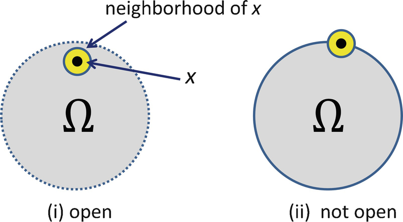
A set that is open, and a set that is not open
Definition 4.4 Let Ω be a subset of a metric space. A covering of Ω is a finite or countably infinite collection {S i} of open sets such that Ω ⊂⋃iS i. A finite covering is a cover containing a finite number of sets. □
For example, the interval [a, b] is covered by the single open set (a − 𝜖, b + 𝜖) for any 𝜖 > 0. Let  be the set of rational numbers, and for 𝜖 > 0 and
  let B(x, 𝜖) be the open ball with center x and radius 𝜖.
 .2 There is no requirement that the sets in the cover of Ω have identical shape or orientation, as illustrated in Fig. 4.2, which illustrates the covering of a square by six ovals, each of which is an open set.
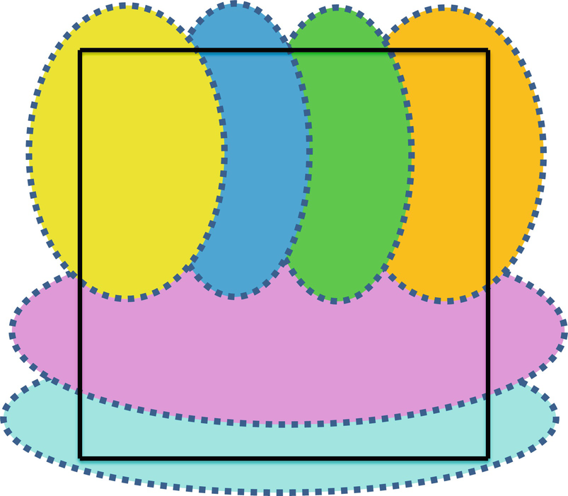
Covering of a square by six open sets
Our second definition of topological dimension, taken from [Eckmann 85], is actually a definition of the covering dimension.
 such that
  for j = 1, 2, …, J and any K + 2 of the
  will have an empty intersection:
Another way of stating this definition, which perhaps is more intuitive, is the following. The topological dimension d
T of a subset Ω of a metric space is the smallest integer K (or ∞) for which the following is true: For every finite covering of Ω by open sets S
1, S
2, …, S
J, one can find another covering  such that
  for j = 1, 2, …, J and each point of Ω is contained in at most K + 1 of the sets
  .
.
 , which have been chosen so that
  and each point of Ω lies in at most 2 of the sets
  . Since this can be done for each finite open cover S
1, S
2, …, S
J, then d
T = 1 for the line segment. □
. Since this can be done for each finite open cover S
1, S
2, …, S
J, then d
T = 1 for the line segment. □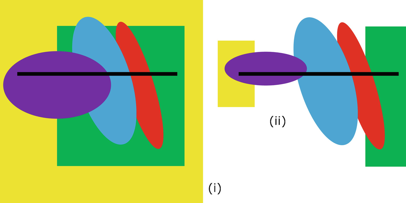
Line segment has d T = 1
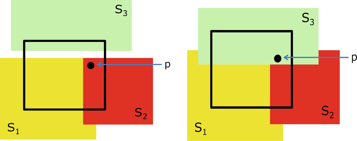
Topological dimension of a square
 satisfying
  we can always find a point p such that
  . If we cover the square with the 4 sets shown in Fig. 4.5, then each point in the square is contained in at most 3 of the S
j, and S
1 ∩ S
2 ∩ S
3 ∩ S
4 = ∅. □
. If we cover the square with the 4 sets shown in Fig. 4.5, then each point in the square is contained in at most 3 of the S
j, and S
1 ∩ S
2 ∩ S
3 ∩ S
4 = ∅. □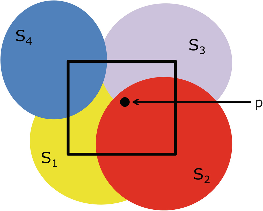
Covering a square by 4 sets
As a final example of Definition 4.5, a solid cube in  has d
T = 3 because in any covering of the cube by smaller cubes there always exists a point belonging to at most four of the smaller cubes. Clearly, Definition 4.5 of d
T does not lend itself to numerical computation. Indeed, [Farmer 82] gave short shrift to topological dimension, noting that he knows of no general analytic or numerical methods to compute d
T, which makes it difficult to apply d
T to studies of dynamical systems.
has d
T = 3 because in any covering of the cube by smaller cubes there always exists a point belonging to at most four of the smaller cubes. Clearly, Definition 4.5 of d
T does not lend itself to numerical computation. Indeed, [Farmer 82] gave short shrift to topological dimension, noting that he knows of no general analytic or numerical methods to compute d
T, which makes it difficult to apply d
T to studies of dynamical systems.
Dimension theory is a branch of topology devoted to the definition and study of of dimension in certain classes of topological spaces. It originated in the early [1920s] and rapidly developed during the next fifteen years. The investigations of that period were concentrated almost exclusively on separable metric spaces ⋯ .3 After the initial impetus, dimension theory was at a standstill for ten years or more. A fresh start was made at the beginning of the fifties, when it was discovered that many results obtained for separable metric spaces can be extended to larger classes of spaces, provided that the dimension is properly defined. ⋯ It is possible to define the dimension of a topological space
in three different ways, the small inductive dimension ind
, the large inductive dimension Ind
, and the covering dimension dim
. ⋯ The covering dimension dim was formally introduced in [a 1933 paper by Čech] and is related to a property of covers of the n-cube I n discovered by Lebesgue in 1911. The three-dimension functions coincide in the class of separable metric spaces, i.e., ind
= Ind
= dim
for every separable metric space
. In larger classes of spaces, the dimensions ind, Ind, and dim diverge. At first, the small inductive dimension ind was chiefly used; this notion has a great intuitive appeal and leads quickly and economically to an elegant theory. [It was later realized that] the dimension ind is practically of no importance outside of the class of separable metric spaces and that the dimension dim prevails over the dimension Ind. ⋯ The greatest achievement in dimension theory during the fifties was the discovery that Ind
= dim
for every metric space
.
To conclude this section, we note that some authors have used a very different definition of “topological dimension”. For example, [Mizrach 92] wrote that Ω has topological dimension d
T if subsets of Ω of size s have a “mass”
that is proportional to  . Thus a square of side length s has a “mass” (i.e., area) of s
2 and a cube of side s has a “mass” (i.e., volume) of d
3, so the square has d
T = 2 and the cube has d
T = 3. We will use a definition of this form when we consider the correlation dimension d
C (Chap. 9) and the network mass dimension d
M (Chap. 12). It is not unusual to see different authors use different names to refer to the same definition of dimension; this is particularly true in the fractal dimension literature.
. Thus a square of side length s has a “mass” (i.e., area) of s
2 and a cube of side s has a “mass” (i.e., volume) of d
3, so the square has d
T = 2 and the cube has d
T = 3. We will use a definition of this form when we consider the correlation dimension d
C (Chap. 9) and the network mass dimension d
M (Chap. 12). It is not unusual to see different authors use different names to refer to the same definition of dimension; this is particularly true in the fractal dimension literature.
4.2 Box Counting Dimension

Box counting for a line and for a square
Now consider a two-dimensional square with side length L. We cover the large square by squares of side length s, where s ≪ L, as illustrated in Fig. 4.6(ii). The number B(s) of small squares needed is given by B(s) = ⌈L 2∕s 2⌉≈ L 2s −2. Since the exponent of s in B(s) = Ls −2 is − 2, we say that the square has box counting dimension 2. Now consider an E-dimensional hypercube with side length L, where E is a positive integer. For s ≪ L, the number B(s) of hypercubes of side length s needed to cover the large hypercube is B(s) = ⌈L E∕s E⌉≈ L Es −E, so the E-dimensional hypercube has box counting dimension E.
We now provide a general definition of the box counting dimension of a geometric object  . By the term “box” we mean an E-dimensional hypercube. By the “linear size” of a box B we mean
the diameter of B (i.e., the
maximal distance between any two points of B), or the maximal variation in any coordinate of B, i.e., maxx,y ∈ Bmax1≤i≤E|x
i − y
i|. By a box of size s we mean a box of linear size s.
A set of boxes is a covering of Ω (i.e., the set of boxes covers Ω) if each point in Ω belongs to at least one box.
. By the term “box” we mean an E-dimensional hypercube. By the “linear size” of a box B we mean
the diameter of B (i.e., the
maximal distance between any two points of B), or the maximal variation in any coordinate of B, i.e., maxx,y ∈ Bmax1≤i≤E|x
i − y
i|. By a box of size s we mean a box of linear size s.
A set of boxes is a covering of Ω (i.e., the set of boxes covers Ω) if each point in Ω belongs to at least one box.

 defined by
 defined by
 then d
B exists, and
then d
B exists, and  . In practice, e.g., when computing the box counting dimension of a digitized image, we need not concern ourselves with the possibility that
  .
.The fact that conditions (i) and (ii) of Definition 4.6 can both be used in (4.1) to define d B is established in [Falconer 03]. In practice, it is often impossible to verify that B(s) satisfies either condition (i) or (ii). The following result provides a computationally extremely useful alternative way to compute d B.
Theorem 4.1 If d B exists, then d B can also be computed using (4.1) where B(s) is the number of boxes that intersect Ω when Ω is covered by a grid of boxes of size s.
 , let
, let  be the number of boxes of size s in some (not necessarily optimal) covering of Ω, and let B(s) be (as usual) the minimal number of boxes of size s required to cover Ω. For s > 0, a box of size s in the E-dimensional grid has the form
 ![$$\displaystyle \begin{aligned}{}[ {x_{{1}}} s, ({x_{{1}}} + 1) s ] \times [ {x_{{2}}} s, ({x_{{2}}} + 1) s ] \times \cdots \times [ {x_{{E}}} s, ({x_{{E}}} + 1) s ] \; , \end{aligned}$$](../images/487758_1_En_4_Chapter/487758_1_En_4_Chapter_TeX_Equi.png)
 .
. and the minimal number B(s) of boxes of size s needed to cover Ω is a non-increasing function of s, then
 . For all sufficiently small positive s we have
  and hence

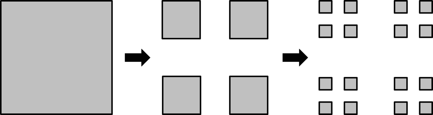
 is contained in at most 3E boxes of size s. To see this, choose an arbitrary point in the set, let B be the box containing that point, and then select the 3E − 1 boxes that are neighbors of B. This is illustrated for E = 2 in Fig. 4.7, which shows a set of size s contained in 32 = 9 boxes of size s; the arbitrarily chosen point is indicated by the small black circle. This yields the inequality
  , from which we obtain


 exists and is equal to d
B. □
exists and is equal to d
B. □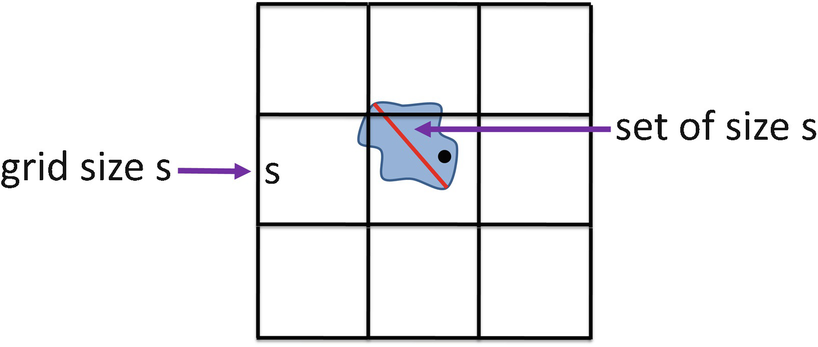
3E boxes cover the set
Thus we can compute d B by counting, for each chosen value of s, the number of boxes that intersect Ω when Ω is covered by a grid of boxes of size s. In practice, for a given s the value B(s) is often computed by picking the minimal B(s) over a set of runs, where each run uses a different offset of the grid (i.e., by shifting the entire grid by a small amount). However, this is time consuming, and usually does not reduce the error by more than 0.5% [Jelinek 98].
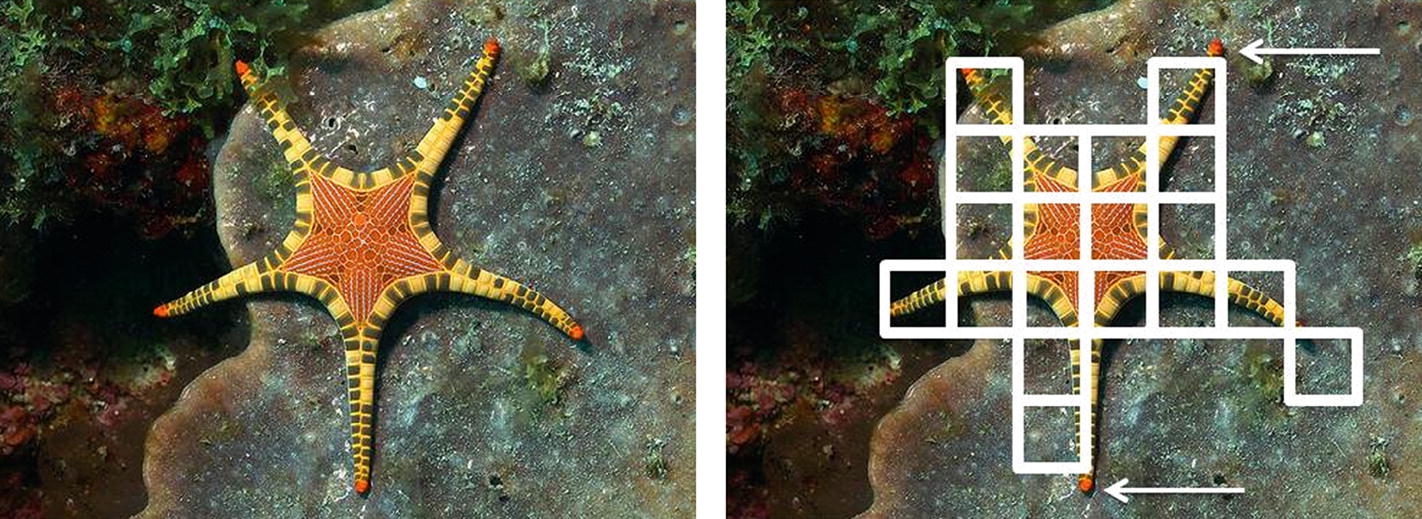
Starfish box counting
In the fractal literature (e.g., [Baker 90, Barnsley 12, Falconer 13, Feder 88, Schroeder 91]) d
B is usually defined assuming that B(s) is either the smallest number of closed balls of radius s needed to cover Ω (i.e., condition (ii) of Definition 4.6), or that B(s) is the number of boxes that intersect Ω when Ω is covered by a grid of boxes of size s (as in Theorem 4.1); both of these choices assume that, for a given s, all boxes have the same size. The definitions of d
B in several well-known books also assume that each box has the same size. All of the examples in this chapter illustrating d
B employ equal-sized boxes. The reason for not defining d
B only in terms of equal-sized boxes is that when we consider, in Chap. 7, the box counting dimension of a complex network  , the boxes that we use to “cover”
  will in general not have the same linear size. Since we will base our definition of d
B of
will in general not have the same linear size. Since we will base our definition of d
B of  on Definition 4.6, we want the definition of d
B for Ω to permit boxes to have different sizes.
on Definition 4.6, we want the definition of d
B for Ω to permit boxes to have different sizes.
In [Falconer 13], a 1928 paper by Georges Bouligand (1889–1979) is credited with introducing box counting; [Falconer 13] also noted that “the idea underlying an equivalent definition had been mentioned rather earlier” by Hermann Minkowski (1984–1909). 5 The “more usual definition” of d B was given by Pontryagin and Schnirelman in 1932 [Falconer 03]. A different historical view, in [Vassilicos 91], is that d B was first defined by Kolmogorov in 1958; indeed, [Vassilicos 91] called d B the Kolmogorov capacity, and observed that the Kolmogorov capacity is often referred to in the literature as the box dimension, similarity dimension, Kolmogorov entropy, or 𝜖-entropy. The use of the term “Kolmogorov capacity” was justified in [Vassilicos 91] by citing [Farmer 83] and a 1989 book by Ruelle.
Another view, in [Lauwerier 91], is that the definition of fractal dimension given by Mandelbrot is a simplification of Hausdorff’s and corresponds exactly with the 1958 definition of Kolmogorov (1903–1987) of the “capacity” of a geometrical figure; in [Lauwerier 91] the term “capacity” was used to refer to the box counting dimension. Further confusion arises since Mandelbrot observed [Mandelbrot 85] that the box counting dimension has been sometimes referred to as the “capacity”, and added that since “capacity” has at least two other quite distinct competing meanings, it should not be used to refer to the box counting dimension. Moreover, [Frigg 10] commented that the box counting dimension has also been called the entropy dimension, e.g., in [Mandelbrot 83b] (p. 359). Fortunately, this babel of terminology has subsided, and the vast majority of recent publications (since 1990 or so) have used the term “box counting dimension”, as we will.
Exercise 4.2 Let f(x) be defined on the positive integers, and let L be the length of the piecewise linear curve obtained by connecting the point (i, f(i)) to the point (i + 1, f(i + 1)) for i = 1, 2, …, N − 1. Show that d
B of this curve can be approximated by  . □
. □
 . By (4.1), the existence of d
B does imply that for each 𝜖 > 0 there is an
. By (4.1), the existence of d
B does imply that for each 𝜖 > 0 there is an  such that for
  we have
 for s > 0. Then
  so
so 

 . Since the minimal number B(s) of boxes of size s needed to cover the coast is given by B(s) ≈ L(s)∕s, then
In the above application of box counting to a starfish, a box is counted if it has a non-empty intersection with the starfish. More generally, in applying Theorem 4.1 to compute d B of Ω, a box is counted if it has a non-empty intersection with Ω. The amount of intersection (e.g., the area of the intersection in the starfish example) is irrelevant. For other fractal dimensions such as the information dimension (Chap. 14) and the generalized dimensions (Chap. 16), the amount of intersection is significant, since “dense” regions of the object are weighted differently than “sparse” regions of the object. The adjective “morphological” is used in [Kinsner 07] to describe a dimension, such as the box counting dimension, which is a purely shape-related concept, concerned only with the geometry of an object, and which utilizes no information about the distribution of a measure over space, or the behavior of a dynamical system over time. Having now discussed both the topological dimension d T and the box counting dimension d B, we can present the definition of a fractal given in [Farmer 82]; he attributed this definition to [Mandelbrot 77].
Definition 4.7 A set is a fractal if its box counting dimension exceeds its topological dimension. □

Six iterations of the Hilbert curve
4.3 A Deeper Dive into Box Counting
 . The problem with this approach is the very slow convergence of
  to d
B [Theiler 90]. To see this, assume
to d
B [Theiler 90]. To see this, assume  holds for some constant c. Then
 versus
  curve is approximately linear is identified. The slope of the curve over this range is an estimate of d
B.
curve is approximately linear is identified. The slope of the curve over this range is an estimate of d
B. space, consider the Sierpiński carpet. The construction of this fractal starts with the filled-in unit square. Referring to Fig. 4.10, the first generation of the construction removes the center 1∕9 of the unit square. What remains is the shaded part of Fig. 4.10(i). This shaded area is covered by 8 of the small squares. Since the side length of the small squares is 1/3, then s = 1∕3 and B(1∕3) = 8. In generation 2, we consider each of the 8 small squares produced in generation 1. For each small square, we remove the center 1∕9 of the square. The result of the generation 2 construction is illustrated in (ii). The shaded area in (ii) is covered by 82 squares of side length 1∕9. Since each small square now has side length 1∕9, then s = 1∕9 and B(1∕9) = 82. In each subsequent iteration, we remove the center 1∕9 of each square sub-region. The slope of the line through
  and
and  is
is 
 .
.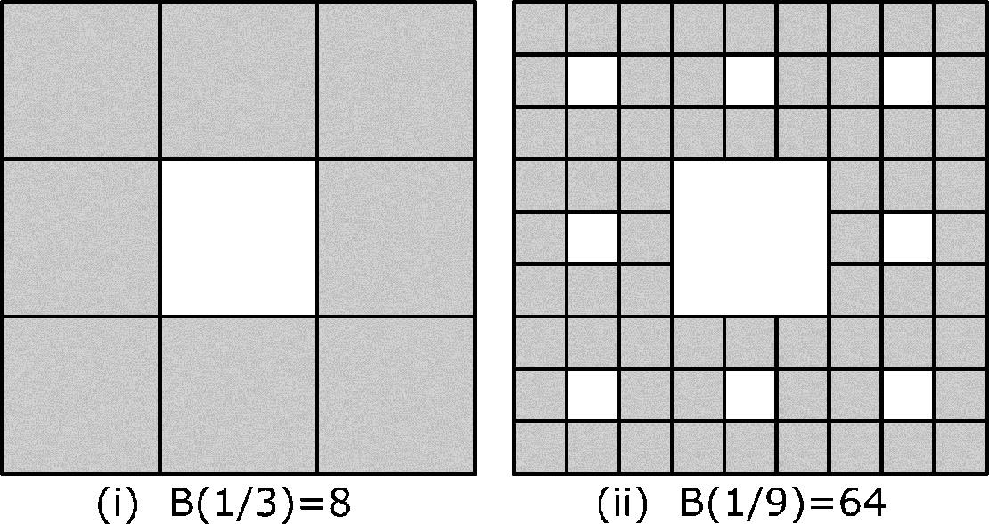
Two generations of the Sierpiński carpet
Exercise 4.3 The above calculation of d
B just used the two box sizes s = 1∕3 and s = 1∕9. Show that  is obtained using any two powers of the box size 1∕3. □
 .
.
Randomized Sierpiński carpet
 and
and  is
is 
 . □
. □
Cantor dust
Example 4.5 As an example of a set for which the box-counting method behaves badly [Falconer 03], consider the set  . This is a bounded countably infinite set. Although we might expect the box counting dimension of Ω to be 0, in fact it is 1∕2. To see this, pick s < 1∕2 and let k be the integer such that
  . Then
  , so
, so  . Similarly
  implies
  .
.
 . For k ≥ 2, the distance between consecutive terms in Ω
k is at least
. For k ≥ 2, the distance between consecutive terms in Ω
k is at least  . Thus a box of size s can cover at most one point of Ω
k, so k boxes are required to cover Ω
k. This implies
. Thus a box of size s can cover at most one point of Ω
k, so k boxes are required to cover Ω
k. This implies 
 .
. then k + 1 boxes of size s cover the interval
 ![$$[0, \frac {1}{k}]$$](../images/487758_1_En_4_Chapter/487758_1_En_4_Chapter_TeX_IEq106.png) . These k + 1 boxes do not cover the k − 1 points
. These k + 1 boxes do not cover the k − 1 points  , but these k − 1 points can be covered by another k − 1 boxes. Hence B(s) ≤ (k + 1) + (k − 1) = 2k and
 . Thus for
  we have
  , so the box counting dimension of this countably infinite set is 1/2. □
The fact that d
B = 1∕2 for  violates one of the properties that should be satisfied by any definition of dimension, namely the property that the dimension of any finite or countably infinite set should be zero. This violation does not occur for the Hausdorff dimension (Chap. 5). Such theoretical problems with the box counting dimension have spurred alternatives to the box counting dimension, as discussed in [Falconer 03]. In practice, these theoretical issues have not impeded the widespread application of box counting (Sect. 6.5).


4.4 Fuzzy Fractal Dimension
If the box-counting method is applied to a 2-dimensional array of pixels, membership is binary: a pixel is either contained in a given box B, or it is not contained in B. The fuzzy box counting dimension is a variant of d B in which binary membership is replaced by fuzzy membership: a “membership function” assigns to a pixel a value in [0, 1] indicating the degree to which the pixel belongs to B. Similarly, for a 3-dimensional array of voxels, binary membership is replaced by assigning a value in [0, 1] indicating the degree to which the voxel belongs to B.8
 of boxes of a given size s, and consider a given box B in the covering. Let
  be the set of pixels covered by B. Whereas for “classical” box counting we count B if
  is non-empty, for fuzzy box counting we compute
 versus
  is roughly linear over a range of s, the slope of the line is the estimate of the fuzzy box counting dimension.
 of all pixels within a given radius of a given pixel j, where we might define the distance between two pixels
to be the distance between the pixel centers. Instead of (4.8), we calculate
of all pixels within a given radius of a given pixel j, where we might define the distance between two pixels
to be the distance between the pixel centers. Instead of (4.8), we calculate 
 versus
  is roughly linear over a range of s, the slope of the line is the estimate of the local fuzzy box counting dimension in the neighborhood
  of pixel j.
4.5 Minkowski Dimension
 and
and  , let dist(x, y) be the Euclidean distance between x and y. For r > 0, the set
Example 4.6 Let E = 3 and let Ω be the single point x. Then d
T = 0 and Ω
r is the closed ball (in  ) of radius r centered at x. We have
  for some constant c
0, so
for some constant c
0, so  . □
. □
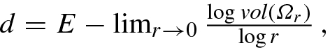
Example 4.7 Let E = 3 and let Ω be a line (straight or curved). Then Ω
r is a “sausage” of diameter 2r (except at the ends) traced by the closed balls (in  ) whose centers follow the line. This construction is a standard method used by mathematicians to “tame” a wildly irregular curve [Mandelbrot 83b]. If Ω is a straight line segment of length L, then d
T = 1 and
) whose centers follow the line. This construction is a standard method used by mathematicians to “tame” a wildly irregular curve [Mandelbrot 83b]. If Ω is a straight line segment of length L, then d
T = 1 and  for come constant c
1, so
for come constant c
1, so  . □
. □
Example 4.8 Let E = 3 and let Ω be a flat 2-dimensional sheet. Then Ω
r is a “thickening” of Ω. If the area of Ω is A, then d
T = 2 and  for some constant c
2, so
for some constant c
2, so  . □
. □
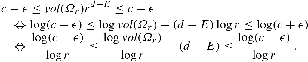
 and consider vol(Ω
r)∕r
E−d as r → 0. Suppose for some nonnegative d the limit
and consider vol(Ω
r)∕r
E−d as r → 0. Suppose for some nonnegative d the limit 
The three examples above considered the Minkowski dimension of a point, line segment, and flat region, viewed as subsets of  . We can also consider their Minkowski dimensions as subsets of
  , in which case we replace “volume” with “area”.
 for a curve and for a straight line of length L. Since now E = 2, the Minkowski dimension d
K of a straight line of length L is
for a curve and for a straight line of length L. Since now E = 2, the Minkowski dimension d
K of a straight line of length L is 

Minkowski sausage in two dimensions
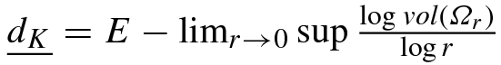
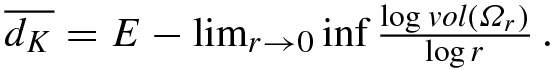
 , defined by (4.2), is equal to
  , and that the upper box counting dimension
  , defined by defined by (4.3), is equal to
  . If
. If  , then the box counting dimension d
B and the Minkowski dimension d
K both exist and d
B = d
K. Thus, while defined differently, the box counting dimension and the Minkowski dimensions, if they exist, are the same. For this reason, the box counting dimension is sometimes called the Minkowski dimension or the Minkowski-Bouligand dimension. In this book we will use d
B when the dimension is computed using (4.1), and d
K when the dimension is computed using (4.10). Although the Minkowski dimension is used much less frequently than the box counting dimension, there are many interesting applications, a few of which we describe below.
, then the box counting dimension d
B and the Minkowski dimension d
K both exist and d
B = d
K. Thus, while defined differently, the box counting dimension and the Minkowski dimensions, if they exist, are the same. For this reason, the box counting dimension is sometimes called the Minkowski dimension or the Minkowski-Bouligand dimension. In this book we will use d
B when the dimension is computed using (4.1), and d
K when the dimension is computed using (4.10). Although the Minkowski dimension is used much less frequently than the box counting dimension, there are many interesting applications, a few of which we describe below.Estimating People Density: The Minkowski dimension was used in [Marana 99] to estimate the number of people in an area. This task is usually accomplished using closed-circuit television systems and human observers, and there is a need to automate this task, e.g., to provide real-time reports when the crowd density exceeds a safe level. To calculate d K, a circle of size r was swept continuously along the edges of the image (the edges outline the people). The total area A(r) swept by the circles of radius r was plotted against r on a log–log plot to estimate d K. This method was applied to nearly 300 images from a railway station in London, UK, to classify the crowd density as very low, low, moderate, high, or very high, and achieved about 75% correct classification. However, the method was not able to distinguish between the high and very high crowd densities. □
Texture Analysis of Pixelated Images: Fractal analysis was applied in [Florindo 13] to a color adjacency graph (CAG), which is a way to represent a pixelation of a colored image. They considered the adjacency matrix of the CAG as a geometric object, and computed its Minkowski dimension. □
Cell Biology: The dilation method was used in [Jelinek 98] to estimate the length of the border of a 2-dimensional image of a neuron.
Each pixel on the border of the image was replaced by a circle of radius r centered on that pixel. Structures whose size is less than r were removed. Letting area(r) be the area of the resulting dilation of the border, area(r)∕(2r) is an estimate of the length of the border. A plot of  versus
  yields an estimate of d
K. □
yields an estimate of d
K. □
Acoustics: As described in [Schroeder 91], the Minkowski dimension has applications in acoustics. The story begins in 1910, when the Dutch physicist Hendrik Lorentz
conjectured that the number of resonant modes of an acoustic resonator depends, up to some large frequency f, only on the volume V of the resonator and not its shape. Although the mathematician David Hilbert predicted that this conjecture, which is important in thermodynamics, would not be proved in his lifetime, it was proved by Herman Weyl, who showed that for large f and for resonators with sufficiently smooth but otherwise arbitrary boundaries, the number of resonant modes is (4π∕3)V (f∕c)3, where c is the velocity of sound. For a two-dimensional resonator such as a drum head, the number of resonant modes is πA(f∕c)2, where A is the surface area of the resonator. These formulas were later improved by a correction term involving lower powers of f. If we drop Weyl’s assumption that the boundary of the resonator is smooth, the correction term turns out to be  . The reason the Minkowski dimension governs the number of resonant modes of an acoustic resonator is that normal resonance modes need a certain area or volume associated with the boundary. □
![$$\displaystyle \begin{aligned} \begin{array}{rcl} f(r) &\displaystyle =&\displaystyle \frac { \log [( \mathrm{area of graph dilated by disks of radius} r)/ {r^2}] } { \log (1/r) } \\ &\displaystyle = &\displaystyle 2 - \frac { \log ( \mathrm{area of graph dilated by disks of radius} r) } { \log r } \, . \end{array} \end{aligned} $$](../images/487758_1_En_4_Chapter/487758_1_En_4_Chapter_TeX_Equ19.png)
 , an overestimate of L(r) yields an underestimate of d. The degree of underestimation depends on the number of end points and the image complexity. To eliminate the underestimation of d
K, specially designed “anisotropic” shapes, to be used at the open ends of such figures, were proposed in [Eins 95].
, an overestimate of L(r) yields an underestimate of d. The degree of underestimation depends on the number of end points and the image complexity. To eliminate the underestimation of d
K, specially designed “anisotropic” shapes, to be used at the open ends of such figures, were proposed in [Eins 95].
astrocytes
Statistical issues in estimating d
K were considered in [Hall 93] for the curve X(t) over the interval 0 < t < 1, where X(t) is a stochastic process observed at N regularly spaced points. Group these N points into J contiguous blocks of width r. Let  be the points in block j and define
  and
and  . Then A =∑1≤j≤Jr (U
j − L
j) is an approximation to the area of the dilation Ω
r, and
. Then A =∑1≤j≤Jr (U
j − L
j) is an approximation to the area of the dilation Ω
r, and  estimates d
K. It was shown in [Hall 93] that this estimator suffers from excessive bias, and a regression-based estimator based on least squares was proposed.11
estimates d
K. It was shown in [Hall 93] that this estimator suffers from excessive bias, and a regression-based estimator based on least squares was proposed.11