I’ve looked at clouds from both sides now
From up and down and still somehow it’s cloud illusions I recall
I really don’t know clouds at all
from “Both Sides, Now” (1969) by Joni Mitchell (1943- ), Canadian singer and songwriter.
A short history of fractals was provided in [Falconer 13]; some of this history was given in the beginning pages of Chap. 1. Fractal geometry was “officially born” in 1975, with the first edition of the book Les Objects Fractals [Mandelbrot 75] by Benoit Mandelbrot (1924–2010); see [Lesmoir 10] for a brief obituary. The word fractal, coined by Mandelbrot, is derived from the Latin fractus, meaning fragmented. A fractal object typically exhibits self-similar behavior, which means the pattern of the fractal object is repeated at different scale lengths, whether these different scales arise from expansion (zooming out) or contraction (zooming in). In 1983, Mandelbrot wrote [Mandelbrot 83a] “Loosely, a ‘fractal set’ is one whose detailed structure is a reduced-scale (and perhaps deformed) image of its overall shape”. Six years later [Mandelbrot 89], he wrote, and preserving his use of italics, “… fractals are shapes whose roughness and fragmentation neither tend to vanish, nor fluctuate up and down, but remain essentially unchanged as one zooms in continually and examination is refined”. In [Lauwerier 91], fractals are defined as “geometric figures with a built-in self-similarity”. However, as we will see in Chaps. 18 and 21, fractality and self-similarity are distinct notions for a network.
3.1 Introduction to Fractals

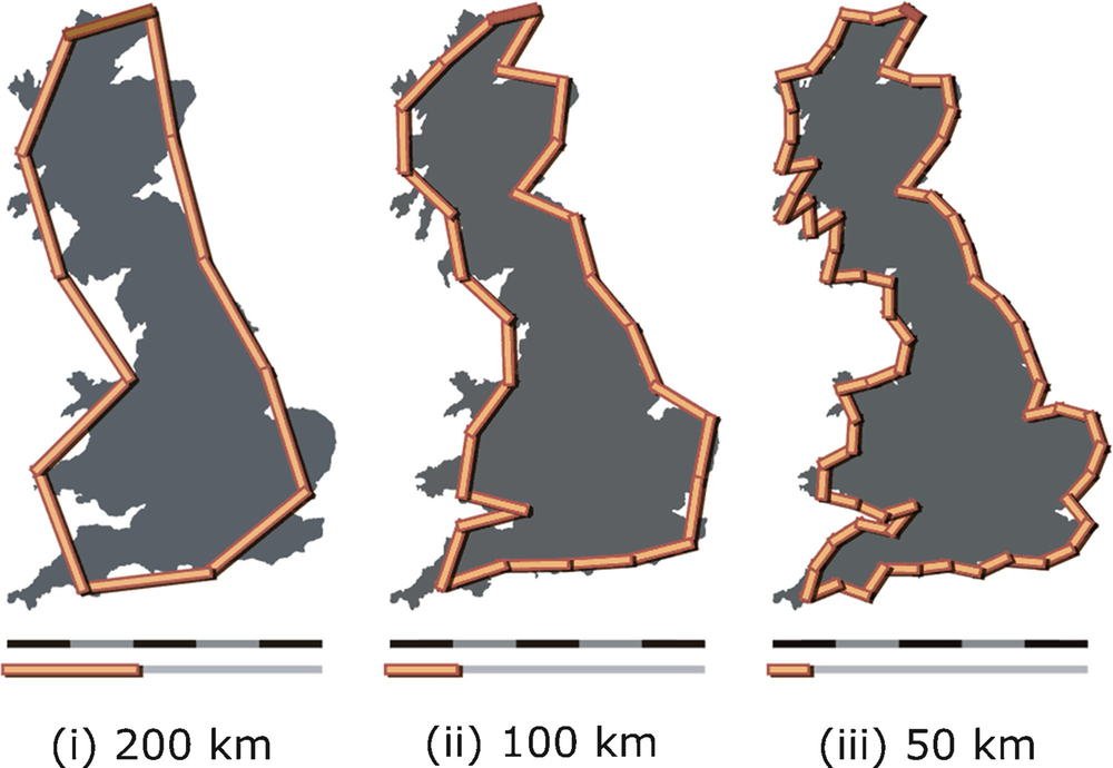
Length of the coast of Britain
To derive the Richardson relation (3.1), let B(s) be the number of ruler lengths of a ruler of length s that are needed to measure the coastline. Then L(s) = sB(s). Assume that B(s) satisfies the relation B(s) = L
0s
−d for some positive constants L
0 and d. Then L(s) = sB(s) = sL
0s
−d = L
0s
1−d, so the equation  describes a straight line with slope 1 − d. From the
  values for various choices of s, we can obtain (e.g., using regression) an estimate of 1 − d and hence d. This technique of stepping along the contour of an object (e.g., a coastline) with a ruler of increasingly finer resolution (i.e., smaller s) to generate the
  values is known as the divider method of determining the fractal dimension.
Exercise 3.1 The extension of Richardson’s relation L(s) ≈ L
0s
1−d to two dimensions is  for some constant
  . Derive this relation. □
As to the actual dimension d of coastlines, the dimension of the coast of Britain was empirically determined to be 1.25. The dimension of other frontiers computed by Richardson and supplied in [Mandelbrot 67] are 1.15 for the land frontier of Germany as of about A.D. 1899, 1.14 for the frontier between Spain and Portugal, 1.13 for the Australian coast, and 1.02 for the coast of South Africa, which appeared in an atlas to be the smoothest. The coast of Britain was chosen for the title of the paper because it looked like one of the most irregular in the world. The application of Richardson’s formula (3.1) to caves was considered in [Curl 86]. One difficulty in applying (3.1) to caves is defining the length of a cave: since a cave is a subterranean volume, the length will be greater for a smaller explorer (who can squeeze into small spaces) than for a large explorer.
Steinhaus also wrote, with great foresight,the left bank of the Vistula, when measured with increased precision, would furnish lengths ten, a hundred, or even a thousand times as great as the length read off the school map.
… a statement nearly adequate to reality would be to call most arcs encountered in nature not rectifiable.4 This statement is contrary to the belief that not rectifiable arcs are an invention of mathematics and that natural arcs are rectifiable: it is the opposite that is true.
Mandelbrot modelled Richardson’s empirical result by first considering the decomposition of an E-dimensional hypercube, with side length L, into K smaller E-dimensional hypercubes. (Mandelbrot actually considered rectangular parallelepipeds, but for simplicity of exposition we consider hypercubes.) The volume of the original hypercube is L
E, the volume of each of the K smaller hypercubes is L
E∕K, and the side length of each of the K smaller hypercubes is (L
E∕K)1∕E = LK
−1∕E. Assume K is chosen so that K
1∕E is a positive integer (e.g., if E = 3, then K = 8 or 27). Let α be the ratio of the side length of each smaller hypercube to the side length of the original hypercube. Then α = LK
−1∕E∕L = K
−1∕E; since K
1∕E > 1 then α < 1. Rewriting α = K
−1∕E as  provides our first fractal dimension definition.
Definition 3.1 [Mandelbrot 67] If an arbitrary geometric object can be exactly decomposed into K parts, such that each of the parts is deducible from the whole by a similarity of ratio α, or perhaps by a similarity followed by rotation and even symmetry, then the similarity dimension of the object is
 . □
. □
![$$\varOmega _1 = [0,{\tfrac {1}{3}}] \cup [{\tfrac {2}{3}},1]$$](../images/487758_1_En_3_Chapter/487758_1_En_3_Chapter_TeX_IEq9.png) . In generation 2 (the “t = 2” row), we remove the middle third of each of the two generation-1 segments, there are now 22 segments, each of length 1∕32 and
. In generation 2 (the “t = 2” row), we remove the middle third of each of the two generation-1 segments, there are now 22 segments, each of length 1∕32 and  . In generation t, we remove the middle third of each of the 2t−1 segments created in generation t − 1, so there are now 2t segments, each of length 1∕3t, and
  . By construction,
 belonging to Ω
t, and observe how in the next generation the middle third of
belonging to Ω
t, and observe how in the next generation the middle third of  is removed, the only way we can tell in which generation
  was created is to measure its length. Since Ω
t is self-similar, we can apply Definition 3.1. In each generation each line segment is divided into thirds, so α = 1∕3. We take two of these thirds, so K = 2. Hence the similarity dimension of the Cantor set is
was created is to measure its length. Since Ω
t is self-similar, we can apply Definition 3.1. In each generation each line segment is divided into thirds, so α = 1∕3. We take two of these thirds, so K = 2. Hence the similarity dimension of the Cantor set is  .
.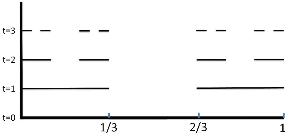
Three generations of the Cantor set
Since we have constructed only t generations of the Cantor set, we call the resulting figure Ω t a pre-fractal. Only in the limit as t →∞ is the resulting object a true fractal. In the real world, we cannot have an infinite number of generations, since we would bump into atomic limits, so each self-similar real-world object would properly be called a “pre-fractal” and not a “fractal”. In practice, this distinction is typically lost, and a self-similar real-world object is typically called a fractal; we will conform to this popular usage.
Fractals are useful when classical Euclidean geometry is insufficient for describing an object. For example, the canopy of a tree
is well modelled by a fractal [Halley 04]: while a cone is the appropriate Euclidean model of the canopy of a tree, the volume in  occupied by a tree canopy is much lower than the volume occupied by a cone, and the surface area of a tree canopy is much higher than that of a cone. A crumbled-up wad of paper has a fractal dimension of about 2.5, the system of arteries in the human body has a dimension about 2.7 [Briggs 92], and the human lung alveolar surface has a fractal dimension of 2.17 [Rigaut 90].5 A fractal dimension of an object provides information about how much the object fills up the space in which it is embedded, which is
  for the crumbled-up wad of paper, the arteries in the human hand, and the human lung.
Determining the fractal dimension of a self-similar feature is generally easier than determining the fractal dimension of a self-affine feature … . Determining whether a one-dimensional feature is self-affine is also a simpler process. If one can interchange or rotate the axes of the coordinate system used to map the feature without producing any fundamental changes, then the feature has the minimum requirements for self-similarity. For example, exchanging the (x, y) values which define a contour line alters nothing essential – both sets of axes carry the same information. However, one cannot exchange the (x, y) values of a topographic profile – even though both axes may be measured in the same units – since the vertical axis integrates different information (i.e., gravity) than does the horizontal axis. Even more obviously, the trace of a particle through time has axes which represent different information (time and distance). More formally, with self-affine fractals the variation in one direction scales differently than the variation in another direction [Mandelbrot 85].
 . The comments in square brackets are this author’s, not Falconer’s; these comments indicate the extent to which Falconer’s characteristics apply to networks, and are intended to pique the reader’s interest rather than to provide formal results.
 - 1.
Ω has a fine structure, i.e., detail on arbitrarily small scales. Just as this is not true for real-world fractals, this is not true for finite networks. The network analogue of structure on an arbitrarily small scale is an infinite network (Chap. 12 ).
- 2.
Ω is too irregular to be described in traditional geometrical language, both locally and globally. The box counting, correlation, information, and generalized dimensions are four global metrics (i.e., calculated using all of Ω or
 ) that characterize a geometric object or a network. Geometric objects and networks can also be described from a “local” perspective, using the “pointwise dimension” (Sect.
9.2
).
) that characterize a geometric object or a network. Geometric objects and networks can also be described from a “local” perspective, using the “pointwise dimension” (Sect.
9.2
). - 3.
Often Ω has some form of self-similarity, perhaps approximate or statistical. For some networks, the self-similarity can be discerned via renormalization (Chap. 21 ). However, network fractality and self-similarity are distinct concepts (Sect. 21.4 ), and we can calculate fractal dimensions of a network not exhibiting self-similarity.
- 4.
Usually, a fractal dimension of Ω (defined in some way) exceeds its topological dimension. The topological dimension of a geometric object is considered in Sect. 4.1 . There is no analogous statement that a fractal dimension of
 (defined in some way) exceeds its topological dimension, since there is no standard notion of a topological dimension of networks. Some definitions of non-fractal dimensions of a network are presented in Chap.
22
.
(defined in some way) exceeds its topological dimension, since there is no standard notion of a topological dimension of networks. Some definitions of non-fractal dimensions of a network are presented in Chap.
22
. - 5.
In most cases of interest, Ω is defined in a very simple way, perhaps recursively. Recursive constructions for generating an infinite network, and the fractal dimensions of such networks, are considered in Chaps. 11 and 12 .
3.2 Fractals and Power Laws
The scaling (1.1) that bulk ∼size d shows the connection between fractality and a power-law relationship. However, as emphasized in [Schroeder 91], a power-law relationship does not necessarily imply a fractal structure. As a trivial example, the distance travelled in time t by a mass initially at rest and subjected to the constant acceleration a is at 2∕2, yet nobody would call the exponent 2 a “fractal dimension”. The Stellpflug formula relating weight and radius of pumpkins is weight = k ⋅radius 2.78, yet no one would say a pumpkin is a fractal. A pumpkin is a roughly spherical shell enclosing an empty cavity, but a pumpkin clearly is not made up of smaller pumpkins.
To study emergent ecological systems, [Brown 02] examined self-similar (“fractal-like”) scaling relationships that follow the power law y = βx α, and showed that power laws reflect universal principles governing the structure and dynamics of complex ecological systems, and that power laws offer insight into how the laws governing the natural sciences give rise to emergent features of biodiversity. The goal of [Brown 02] was similar to the goal of [Barabási 09], which showed that processes such as growth with preferential attachment (Sect. 2.4) give rise to scaling laws that have wide application. In [Brown 02] it was also observed that scaling patterns are mathematical descriptions of natural patterns, but not scientific laws, since scaling patterns do not describe the processes that spawn these patterns. For example, spiral patterns of stars in a galaxy are not physical laws but the results of physical laws operating in complex systems.
Other examples, outside of biology, of power laws are the frequency distribution of earthquake sizes, the distribution of words in written languages, and the distribution of the wealth of nations. A few particularly interesting power laws are described below. For some of these examples, e.g., Kleiber’s Law, the exponent of the power law may be considered a fractal dimension if it arises from self-similarity or other fractal analysis.
Zipf’s Law: One of the most celebrated power laws in the social sciences is Zipf’s Law, named after Harvard professor George Kingsley Zipf (1902–1950). The law says that if N items are ranked in order of most common (n = 1) to least common (n = N), then the frequency of item n is proportional to 1/n d, where d is the Zipf dimension. This relationship has been used, for example, to study the population of cities inside a region. Let N be the number of cities in the region and for n = 1, 2, …, N, let P n be the population of the n-th largest city, so P 1 is the population of the largest of the N cities and P n > P n+1 for n = 1, 2, …, N − 1. Then Zipf’s law predicts P n ∝ n −d. This dimension was computed in [Chen 11] for the top 513 cities in the U.S.A. Observing that the data points on a log–log scale actually follow two trend lines with different slopes, the computed value in [Chen 11] is d = 0.763 for the 32 largest of the 513 cites and d = 1.235 for the remaining 481 cities.
Kleiber’s Law: In the 1930s, the Swiss biologist Max Kleiber empirically determined that for many animals, the basal metabolic rate (the energy expended per unit time by the animal at rest) is proportional to the 3∕4 power of the mass of the animal. This relationship, known as Kleiber’s law, was found to hold over an enormous range of animal sizes, from microbes to blue whales. Kleiber’s law has numerous applications, including calculating the correct human dose of a medicine tested on mice. Since the mass of a spherical object of radius r scales as r 3, but the surface area scales as r 2, larger animals have less surface area per unit volume than smaller animals, and hence larger animals lose heat more slowly. Thus, as animal size increases, the basal metabolic rate must decrease to prevent the animal from overheating. This reasoning would imply that the metabolic rate scales as mass to the 2∕3 power [Kleiber 14]. Research on why the observed exponent is 3∕4, and not 2∕3, has considered the fractal structure of animal circulatory systems [Kleiber 12].
Exponents that are Multiples of 1/3 or 1/4: Systems characterized by a power law whose exponent α is a multiple of 1∕3 or 1∕4 were studied in [Brown 02]. Multiples of 1∕3 arise in Euclidean scaling: we have α = 1∕3 when the independent variable x is linear, and α = 2∕3 for surface area. Multiples of 1∕4 arise when, in biological allometries, organism lifespans scale with α = 1∕4.6 Organism metabolic rates scale with α = 3∕4 (Kleiber’s Law). Maximum rates of population growth scale with α = −1∕4. In [Brown 02], the pervasive quarter-power scaling (i.e., multiples of 1∕4) in biological systems is connected to the fractal-like designs of resource distribution networks such as rivers. (Fractal dimensions of networks with a tree structure, e.g., rivers, are studied in Sect. 22.1.)
 . Letting p(⋅) denote probability, the law says that for j = 1, 2, …, 9 we have
In the beginning of Chap. 3 we considered a fractal dimension of the coastline of Britain.
The fractal dimension of a curve in  was also used to study Alzheimer’s Disease [Smits 16], using EEG (electroencephalograph) recordings of the brain. Let the EEG readings at N points in time be denoted by y(t
1), y(t
2), …, y(t
N). Let Y (1) be the curve obtained by plotting all N points and joining the adjacent points by a straight line; let Y (2) be the curve obtained by plotting every other point and joining the adjacent points by a straight line; in general, let Y (k) be the curve obtained by plotting every k-th point and joining the points by a straight line. Let L(k) be the length of the curve Y (k). If L(k) ∼ k
−d, then d is called the Higuchi fractal dimension [Smits 16].
This dimension is between 1 and 2, and a higher value indicates higher signal complexity. This study confirmed that this fractal dimension “depends on age in healthy people and is reduced in Alzheimer’s Disease”.
Moreover, this fractal dimension “increases from adolescence to adulthood and decreases from adulthood to old age. This loss of complexity in neural activity is a feature of the aging brain and worsens with Alzheimer’s disease”.
was also used to study Alzheimer’s Disease [Smits 16], using EEG (electroencephalograph) recordings of the brain. Let the EEG readings at N points in time be denoted by y(t
1), y(t
2), …, y(t
N). Let Y (1) be the curve obtained by plotting all N points and joining the adjacent points by a straight line; let Y (2) be the curve obtained by plotting every other point and joining the adjacent points by a straight line; in general, let Y (k) be the curve obtained by plotting every k-th point and joining the points by a straight line. Let L(k) be the length of the curve Y (k). If L(k) ∼ k
−d, then d is called the Higuchi fractal dimension [Smits 16].
This dimension is between 1 and 2, and a higher value indicates higher signal complexity. This study confirmed that this fractal dimension “depends on age in healthy people and is reduced in Alzheimer’s Disease”.
Moreover, this fractal dimension “increases from adolescence to adulthood and decreases from adulthood to old age. This loss of complexity in neural activity is a feature of the aging brain and worsens with Alzheimer’s disease”.
Exercise 3.2 Referring to the above study of Alzheimer’s Disease, is the calculation of the Higuchi dimension an example of the divider method (Sect. 3.1), or is it fundamentally different? □
3.3 Iterated Function Systems
An Iterated Function System (IFS) is a
useful way of describing a self-similar geometric fractal  . An IFS operates on some initial set
  by creating multiple copies of Ω
0 such that each copy is a scaled down version of Ω
0. The multiple copies are then translated and possibly rotated in space so that the overlap of any two copies is at most one point. The set of these translated/rotated multiple copies is Ω
1. We then apply the IFS to each scaled copy in Ω
1, and continue this process indefinitely. Each copy is smaller, by the same ratio, than the set used to create it, and the limit of applying the IFS infinitely many times is the fractal Ω. In this section we show how to describe a self-similar set using an IFS. In the next section, we discuss the convergence of the sets generated by an IFS. Iterated function systems were introduced in [Hutchinson 81] and popularized in [Barnsley 12].7 Besides the enormous importance of iterated function systems for geometric objects, the other reason for presenting (in this section and the following section) IFS theory is that we will encounter an IFS for building an infinite network in Sect. 13.1.
by creating multiple copies of Ω
0 such that each copy is a scaled down version of Ω
0. The multiple copies are then translated and possibly rotated in space so that the overlap of any two copies is at most one point. The set of these translated/rotated multiple copies is Ω
1. We then apply the IFS to each scaled copy in Ω
1, and continue this process indefinitely. Each copy is smaller, by the same ratio, than the set used to create it, and the limit of applying the IFS infinitely many times is the fractal Ω. In this section we show how to describe a self-similar set using an IFS. In the next section, we discuss the convergence of the sets generated by an IFS. Iterated function systems were introduced in [Hutchinson 81] and popularized in [Barnsley 12].7 Besides the enormous importance of iterated function systems for geometric objects, the other reason for presenting (in this section and the following section) IFS theory is that we will encounter an IFS for building an infinite network in Sect. 13.1.
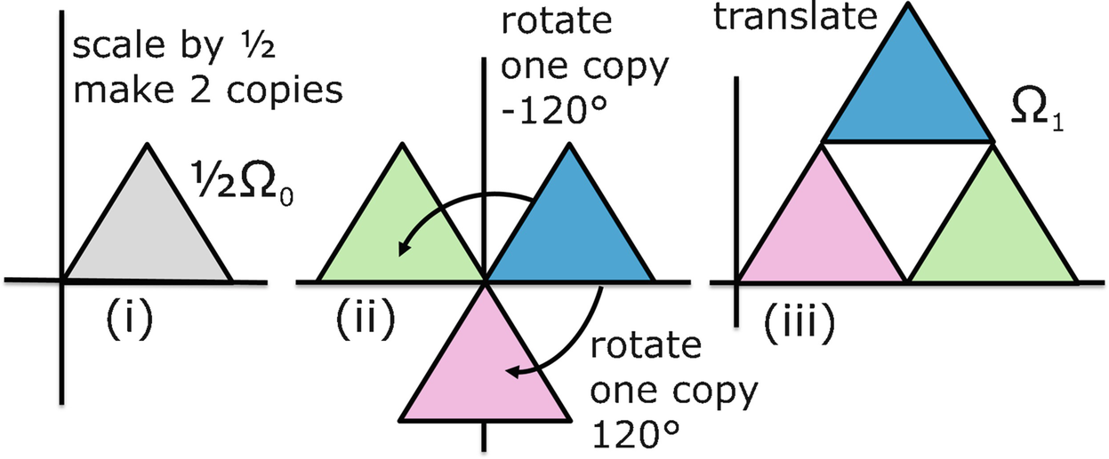
 . Let the bottom left corner of equilateral triangle Ω
0 be the origin (0, 0), let the bottom right corner be (1, 0), and let the top corner be
. Let the bottom left corner of equilateral triangle Ω
0 be the origin (0, 0), let the bottom right corner be (1, 0), and let the top corner be  , so each side length is 1. We first scale Ω
0 by 1∕2 and then make two copies, superimposed on each other, as shown in (i). Then one of the copies is rotated 120∘ clockwise, and the other copy is rotated 120∘ counterclockwise, as shown in (ii). Finally, the two rotated copies are translated to their final position, as shown in (iii), yielding Ω
1. Let the point
, so each side length is 1. We first scale Ω
0 by 1∕2 and then make two copies, superimposed on each other, as shown in (i). Then one of the copies is rotated 120∘ clockwise, and the other copy is rotated 120∘ counterclockwise, as shown in (ii). Finally, the two rotated copies are translated to their final position, as shown in (iii), yielding Ω
1. Let the point  be represented by a column vector (i.e., a matrix
with two rows and one column), so
be represented by a column vector (i.e., a matrix
with two rows and one column), so 


IFS for the Sierpiński triangle


The Sierpiński triangle can also be generated by a simpler IFS that eliminates the need for rotation.


 . The infinite sequence of sets
  is generated using the same recurrence (3.5) with f
1, f
2, and f
3 now defined by (3.6). □
is generated using the same recurrence (3.5) with f
1, f
2, and f
3 now defined by (3.6). □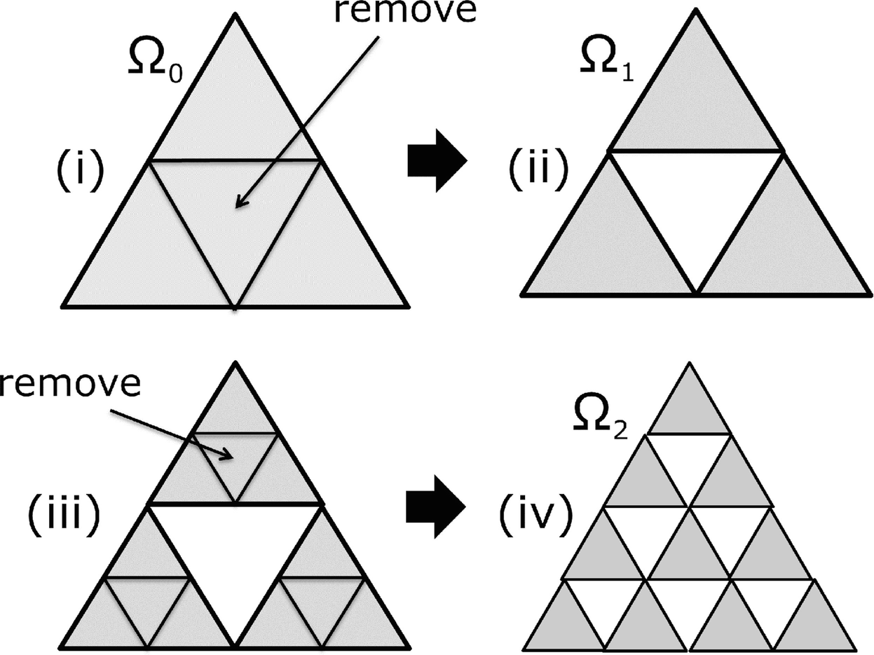
Another IFS for the Sierpiński triangle
 we have f(C) ≡ f
1(C) ∪ f
2(C) ∪ f
3(C). For example, with f
1, f
2, and f
3 defined by either (3.2), (3.3), (3.4) or by (3.6), we have f(Ω
0) = Ω
1. We can now apply f to f(Ω
1), obtaining
we have f(C) ≡ f
1(C) ∪ f
2(C) ∪ f
3(C). For example, with f
1, f
2, and f
3 defined by either (3.2), (3.3), (3.4) or by (3.6), we have f(Ω
0) = Ω
1. We can now apply f to f(Ω
1), obtaining 
 , for t = 3, 4, … . In the next section, we will show that f is a contraction map, which implies that the sequence of sets
  converges to some set Ω, called the attractor of the IFS f. Moreover, Ω depends only on the function f and not on the initial set Ω
0, that is, the sequence of sets
converges to some set Ω, called the attractor of the IFS f. Moreover, Ω depends only on the function f and not on the initial set Ω
0, that is, the sequence of sets  converges to Ω for any non-empty compact set Ω
0.
converges to Ω for any non-empty compact set Ω
0.The use of an IFS to provide a graphic representation of human DNA sequences was discussed in [Berthelsen 92]. DNA is composed of four bases (adenine, thymine, cytosine, and guanine) in strands. A DNA sequence can be represented by points within a square, with each corner of the square representing one of the bases. As described in [Berthelsen 92], “The first point, representing the first base in the sequence, is plotted halfway between the center of the square and the corner representing that base. Each subsequent base is plotted halfway between the previous point and the corner representing the base. The result is a bit-mapped image with sparse areas representing rare subsequences and dense regions representing common subsequences”. While no attempt was made in [Berthelsen 92] to compute a fractal dimension for such a graphic representation, there has been considerable interest in computing fractal dimensions of DNA (Sect. 16.6).
3.4 Convergence of an IFS
Since an IFS operates on a set, and we will be concerned with distances between sets, we need some machinery, beginning with the definition of a metric and metric space, and then the definition of the Hausdorff distance between two sets. The material below is based on [Hepting 91] and [Barnsley 12]. Let  be a space, e.g.,
  .
.
Definition 3.2 A metric is a nonnegative real valued function dist(⋅, ⋅)
defined on  such that the following three conditions hold for each x, y, z in
  :
:
1. dist(x, y) = 0 if and only if x = y,
2. dist(x, y) = dist(y, x),
3. dist(x, y) ≤ dist(y, z) + dist(x, z). □
The second condition imposes symmetry, and the third condition imposes the triangle inequality. Familiar examples of metrics are
1. the “Manhattan” distance
 , known as the L
1 metric,
, known as the L
1 metric,
2. the Euclidean distance
 , known as the L
2 metric,
, known as the L
2 metric,
3. the “infinity” distance
 , known as the L
∞ metric.
, known as the L
∞ metric.
 , the L
1 distance is 7 + 4 = 11, and the L
∞ distance is
, the L
1 distance is 7 + 4 = 11, and the L
∞ distance is  . □
. □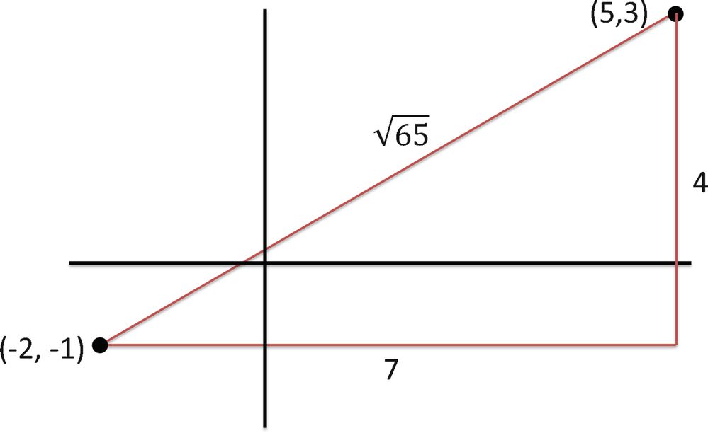
The L 1, L 2, and L ∞ metrics
 . The generalization of the L
1, L
2, and L
∞ metrics is the L
p metric, defined by
. The generalization of the L
1, L
2, and L
∞ metrics is the L
p metric, defined by 
The Euclidean distance is L 2(x, y), the Manhattan distance is L 1(x, y), and the infinity distance is L ∞(x, y). In Chap. 16 on multifractals, we will encounter expressions similar to (3.7).
Exercise 3.3 Show that L ∞ =limp→∞L p. □
Definition 3.3 A metric space  is a space
  equipped with a metric dist(⋅, ⋅). □
The space  need not be Euclidean space. For example,
  could be the space of continuous functions on the interval [a, b]. Letting f and g be two such functions, we could define dist(⋅ , ⋅) by dist(f, g) =maxx ∈ [a,b]| f(x) − g(x) |.
Definition 3.4 Let  be a metric space. Then
  is complete
if for each sequence
is complete
if for each sequence  of points in
  that converges to x we have
  . □
. □
In words, the metric space is complete if the limit of each convergent sequence of points in the space also belongs to the space.8 For example, let  be the half-open interval (0, 1], with dist(x, y) = |x − y|. Then
  is not complete, since the sequence
  converges to 0, but
  . However, if now we let
  be the closed interval [0, 1], then
  is complete, as is
  .
.
Definition 3.5 Let  be a metric space, and let
  . Then Ω is compact
if every sequence {x
i}, i = 1, 2, … contains a subsequence having a limit in Ω. □
. Then Ω is compact
if every sequence {x
i}, i = 1, 2, … contains a subsequence having a limit in Ω. □
For example, a subset of  is compact if and only if it is closed and bounded. Now we can define the space which will be used to study iterated function systems.
Definition 3.6 Given the metric space  , let
, let  denote the space whose points are the non-empty compact subsets of
  . □
. □
For example, if  then a point
  represents a non-empty, closed, and bounded subset of
  . The reason we need
  is that we want to study the behavior of an IFS
which maps a compact set
is that we want to study the behavior of an IFS
which maps a compact set  to two or more copies of Ω, each reduced in size. To study the convergence properties of the IFS, we want to be able to define the distance between two subsets of
  . Thus we need a space whose points are compact subsets of
  and that space is precisely
  . However, Definition 3.6 applies to any metric space
  ; we are not restricted to
  .
.
Now we define the distance between two non-empty compact subsets of  , that is, between two points of
  .
This is known as the Hausdorff distance between two sets.
The definition of the Hausdorff distance requires defining the distance from a point to a set.
.
This is known as the Hausdorff distance between two sets.
The definition of the Hausdorff distance requires defining the distance from a point to a set.
In Definition 3.7 below, we use dist(⋅, ⋅) in two different ways: as the distance dist(x, y) between two points in  , and as the distance dist (x, T) between a point
  and an element
  (i.e., a non-empty compact subset of
  ). Since capital letters are used to denote elements of
  , the meaning of dist (⋅, ⋅) in any context is unambiguous.
 be a complete metric space.
For
be a complete metric space.
For  and
and  , the distance from x to Y
is
, the distance from x to Y
is 
 and
and  , the directed distance
from X to Y is
, the directed distance
from X to Y is 

 , that dist(y
1, X) = dist(y
1, x
1), that dist(y
3, X) = dist(y
3, x
2), and that
, that dist(y
1, X) = dist(y
1, x
1), that dist(y
3, X) = dist(y
3, x
2), and that  . The two directed distances are not equal, since
  . Finally,
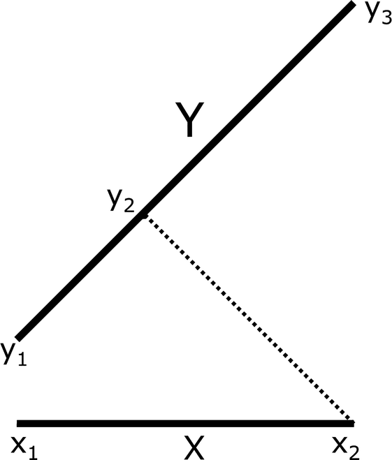
Illustration of Hausdorff distance
It is proved in [Barnsley 12] that if  is a complete metric space, then
  is a complete metric space. The value of this result is that all the results and techniques developed for complete metric spaces, in particular relating to convergent sequences, can be extended to
  with the Hausdorff distance.
First, some notation. Let
with the Hausdorff distance.
First, some notation. Let  and let
  . Define f
1(x) = f(x). For t = 2, 3, …, by f
t(x) we mean
. Define f
1(x) = f(x). For t = 2, 3, …, by f
t(x) we mean  . Thus
  ,
,  , etc.
Definition 3.8 Let  be a metric space. The function
  is a contraction map if for some positive constant α < 1 and all
 we have dist(f(s), f(t)) ≤ α dist(s, t). The constant α is called the contraction factor. □
Definition 3.9 A fixed point of a function  is a point
  such that f(x
⋆) = x
⋆. □
such that f(x
⋆) = x
⋆. □
A proof of the following classical result can be found in [Barnsley 12].
 be a metric space,
and let
be a metric space,
and let  be a contraction map. Then there is exactly one fixed point x
⋆ of f. Moreover, for each
be a contraction map. Then there is exactly one fixed point x
⋆ of f. Moreover, for each  the sequence f
t(x
0) converges, and limt→∞f
t(x
0) = x
⋆. With Theorem 3.1 we can prove, under appropriate assumptions, the convergence of the sets Ω
t generated by an IFS.
Recall that
the sequence f
t(x
0) converges, and limt→∞f
t(x
0) = x
⋆. With Theorem 3.1 we can prove, under appropriate assumptions, the convergence of the sets Ω
t generated by an IFS.
Recall that  is the space of non-empty compact subsets of the metric space
  . For k = 1, 2, …, K, let
  . Assume that each f
k is a contraction map with contraction factor α
k < 1, so
. Assume that each f
k is a contraction map with contraction factor α
k < 1, so 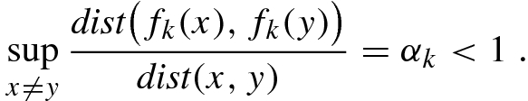
 , define
  by
by 
so f(C) is the union of the K sets f
k(C). Then f is a contraction map, with contraction factor  , and α < 1. By Theorem 3.1, f has a unique fixed point. The fixed point, which we denote by Ω, is an element of
  , so Ω is non-empty and compact, and limt→∞Ω
t = Ω for any choice of Ω
0. We call Ω the attractor of the IFS. The attractor Ω is the unique non-empty solution of the equation f(Ω) = Ω, and
, so Ω is non-empty and compact, and limt→∞Ω
t = Ω for any choice of Ω
0. We call Ω the attractor of the IFS. The attractor Ω is the unique non-empty solution of the equation f(Ω) = Ω, and  .
.
Example 3.
2
(continued) For the iterated function system of Example 3.2, the metric space  is
is  with the Euclidean distance L
2, K = 3, and each f
k has the contraction ratio 1∕2. The attractor is the Sierpiński triangle. □
with the Euclidean distance L
2, K = 3, and each f
k has the contraction ratio 1∕2. The attractor is the Sierpiński triangle. □
Sometimes slightly different terminology [Glass 11] is used to describe an IFS. A function f defined on a metric space  is a similarity
if for some α > 0 and each
is a similarity
if for some α > 0 and each  we have
  . A contracting ratio list
  is a list of numbers such that 0 < α
k < 1 for each k. An iterated function system (IFS) realizing a ratio list
is a list of numbers such that 0 < α
k < 1 for each k. An iterated function system (IFS) realizing a ratio list
 in a metric space
  is a list of functions
  defined on
  such that f
k is a similarity with ratio α
k. A non-empty compact set Ω ⊂ X is an invariant set for an IFS if Ω = f
1(Ω) ∪ f
2(Ω) ∪⋯ ∪ f
K(Ω). Theorem 3.1, the Contraction Mapping Theorem now, can now be stated as: If
such that f
k is a similarity with ratio α
k. A non-empty compact set Ω ⊂ X is an invariant set for an IFS if Ω = f
1(Ω) ∪ f
2(Ω) ∪⋯ ∪ f
K(Ω). Theorem 3.1, the Contraction Mapping Theorem now, can now be stated as: If  is an IFS realizing a contracting ratio list
  then there exists a unique non-empty compact invariant set for the IFS.
The Contraction Mapping Theorem shows that to compute Ω we can start with any set  , and generate the iterates Ω
1 = f(Ω
0), Ω
2 = f(Ω
1), etc. In practice, it may not be easy to determine f(Ω
h), since it may not be easy to represent each f
k(Ω
t) if f
k is a complicated function. Another method of computing Ω is a randomized method, which begins by assigning a positive probability p
k to each of the K functions f
k such that
, and generate the iterates Ω
1 = f(Ω
0), Ω
2 = f(Ω
1), etc. In practice, it may not be easy to determine f(Ω
h), since it may not be easy to represent each f
k(Ω
t) if f
k is a complicated function. Another method of computing Ω is a randomized method, which begins by assigning a positive probability p
k to each of the K functions f
k such that  . Let
. Let  be arbitrary, and set
  . In iteration t of the randomized method, select one of the functions f
k, using the probabilities p
k, select a random point x from the set
. In iteration t of the randomized method, select one of the functions f
k, using the probabilities p
k, select a random point x from the set  , compute f
k(x), and set
, compute f
k(x), and set  .
.
 ,
,  ,
,  , and choose
  , so initially
  . To compute the next point, we roll a “weighted” 3-sided die with probabilities p
1, p
2, p
3. Suppose we select f
2. We compute
. To compute the next point, we roll a “weighted” 3-sided die with probabilities p
1, p
2, p
3. Suppose we select f
2. We compute 
 . We start the next iteration by rolling the die again.