Humankind has not woven the web of life. We are but one thread within it. Whatever we do to the web, we do to ourselves. All things are bound together. All things connect.
Chief Seattle (1786–1866), a leader of the Suquamish and Duwamish Native American tribes in what is now Washington state.
This chapter provides supplemental information on six topics: (i) rectifiable arcs and arc length, to supplement the material on jagged coastlines in the beginning of Chap. 3 and also used in Sect. 6.4 on the box counting dimension of a spiral,
(ii) the Gamma function and hypersphere volumes, used in Sect. 5.1 on the Hausdorff dimension, (iii) Laplace’s method of steepest descent, used in Sect. 16.3 on the spectrum of the multifractal Cantor set, (iv) Stirling’s approximation, used in Sect. 16.3, (v) convex functions and the Legendre transform, used in Sect. 16.4 on multifractals, and (vi) graph spectra (the study of the eigenvectors and eigenvalues of the adjacency matrix
of  ), used in Sect. 20.1.
23.1 Rectifiable Arcs and Arc Length
Rectifiable Arc
 be continuously differentiable on the interval (S, T). Then the length L of the arc of f(x) from S to T is
 ![$$\displaystyle \begin{aligned} \begin{array}{rcl} L = \int_S^T \sqrt{1 + [f^{\prime}(x) ]^2 } \; dx \, . {} \end{array} \end{aligned} $$](../images/487758_1_En_23_Chapter/487758_1_En_23_Chapter_TeX_Equ1.png)
 and
and  . We have
 ![$$\displaystyle \begin{aligned} \begin{array}{rcl} L(x) &\displaystyle =&\displaystyle \sqrt { (dx)^2 + [f(x+dx)-f(x)]^2 } \\ &\displaystyle =&\displaystyle \sqrt { (dx)^2 [ 1 + [\bigl( f(x+dx)-f(x) \bigr)/dx]^2 } \\ &\displaystyle \approx &\displaystyle \sqrt{ 1 + [ f^{\prime}(x) ]^2 } \; dx \, . \end{array} \end{aligned} $$](../images/487758_1_En_23_Chapter/487758_1_En_23_Chapter_TeX_Equ2.png)
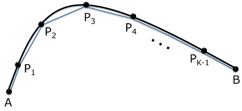
![$$\displaystyle \begin{aligned} \begin{array}{rcl} L &\displaystyle \approx &\displaystyle \sum_{k=0}^{K-1} \sqrt{ 1 + [ f^{\prime}(x_{{k}}) ]^2 } \; dx \, . \end{array} \end{aligned} $$](../images/487758_1_En_23_Chapter/487758_1_En_23_Chapter_TeX_Equ3.png)
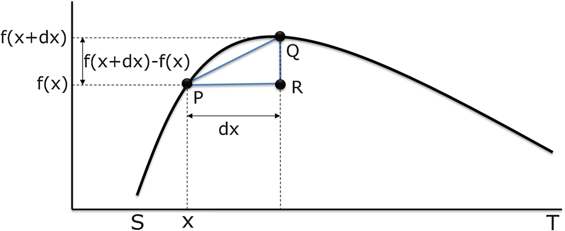
Computing the length of a rectifiable arc

 and
and  , then
  and
and  . From this we obtain, after some algebra,

23.2 The Gamma Function and Hypersphere Volumes


 with radius r is [Manin 06]

 , we have t = u
2 and
, we have t = u
2 and 

 . Using the identity Γ(x + 1) = xΓ(x),
 is
is 
23.3 Laplace’s Method of Steepest Descent

We require three assumptions. Assume that (i) F(λ) exists for all sufficiently large λ; (ii) the functions f and g are twice differentiable on (a, b); and (iii) the minimal value of g over [a, b] is attained at some y ∈ (a, b) satisfying g ′′(y) > 0 and f(y) ≠ 0. Assumption (ii) allows us to replace f and g by their second-order Taylor series expansions. Assumption (iii) implies that g ′(y) = 0 and that g is strictly convex at y, so y is an isolated local minimum of g.
![$$\displaystyle \begin{aligned} \begin{array}{rcl} F(\lambda) &\displaystyle =&\displaystyle e^{-\lambda g(y)} \int_a^b f(x) \, e^{-\lambda[ g(x) - g(y)]} dx \\ &\displaystyle \approx&\displaystyle e^{-\lambda g(y)} \int_{y-\epsilon}^{y+\epsilon} f(x) \, e^{-\lambda[ g(x) - g(y)]} dx \\ &\displaystyle \approx&\displaystyle e^{-\lambda g(y)} f(y) \int_{y-\epsilon}^{y+\epsilon} \, e^{-\lambda[ g(x) - g(y)]} dx \\ &\displaystyle \approx&\displaystyle e^{-\lambda g(y)} f(y) \int_{y-\epsilon}^{y+\epsilon} \, e^{-\lambda[ g^{\, \prime}(y)(x-y) + (1/2) g^{\prime \prime}(y)(x-y)^2]} dx \\ &\displaystyle =&\displaystyle e^{-\lambda g(y)} f(y) \int_{y-\epsilon}^{y+\epsilon} \, e^{-(\lambda/2)g^{\prime \prime}(y)(x-y)^2} dx \\ &\displaystyle \approx&\displaystyle e^{-\lambda g(y)} f(y) \int_{-\infty}^{\infty} \, e^{-(\lambda/2)g^{\prime \prime}(y)(x-y)^2} dx \\ &\displaystyle =&\displaystyle e^{-\lambda g(y)} f(y) \int_{-\infty}^{\infty} \, e^{-(\lambda/2)g^{\prime \prime}(y)z^2]} dz \\ &\displaystyle =&\displaystyle e^{-\lambda g(y)} f(y) \sqrt{ \frac{2 \pi}{\lambda g^{\prime \prime}(y)} } \end{array} \end{aligned} $$](../images/487758_1_En_23_Chapter/487758_1_En_23_Chapter_TeX_Equ10.png)


23.4 Stirling’s Approximation
 for large n, and often this is referred to as Stirling’s approximation.
The actual approximation credited to Stirling is
for large n, and often this is referred to as Stirling’s approximation.
The actual approximation credited to Stirling is 
![$$\displaystyle \begin{aligned} \begin{array}{rcl} \varGamma(x+1) &\displaystyle =&\displaystyle \int_{t=0}^{\infty} t^{x} \, e^{-t} dt \\ &\displaystyle = &\displaystyle \int_{t=0}^{\infty} e^{x \ln t} \, e^{-t} dt \\ &\displaystyle = &\displaystyle \int_{t=0}^{\infty} e^{-x[(t/x) - \ln t]} dt \\ &\displaystyle = &\displaystyle x \int_{z=0}^{\infty} e^{-x[z - \ln(xz)]} dz \;\;\;\;\; \mbox{(using } t=xz\mbox{)} \\ &\displaystyle = &\displaystyle x e^{x \ln x} \int_{z=0}^{\infty} e^{-x(z - \ln z)} dz \\ &\displaystyle = &\displaystyle x^{x +1} \int_{z=0}^{\infty} e^{-x(z - \ln z)} dz \end{array} \end{aligned} $$](../images/487758_1_En_23_Chapter/487758_1_En_23_Chapter_TeX_Equ13.png)

 . The point z = 1 is the unique global minimum of g(z) over {z | z > 0}, and g(1) = 1, g
′(1) = 0, and g
′′(1) = 1. Since all three assumptions of Sect. 23.3 are satisfied, by (23.6) we have, as x →∞,
. The point z = 1 is the unique global minimum of g(z) over {z | z > 0}, and g(1) = 1, g
′(1) = 0, and g
′′(1) = 1. Since all three assumptions of Sect. 23.3 are satisfied, by (23.6) we have, as x →∞, 

Exercise 23.1 Plot the error incurred by using (23.7) to approximate n! as a function of the positive integer n. □
23.5 Convex Functions and the Legendre Transform
 be convex. For simplicity, assume for the remainder of this section that (i) F is twice differentiable and (ii) F
′′(x) > 0 for all x. These two assumptions imply that F is strictly convex and that F
′(x) is monotone increasing with x.2 For this discussion it is important to distinguish between the function F and the value F(x) of the function at the point x. Since F is differentiable and convex, then
be convex. For simplicity, assume for the remainder of this section that (i) F is twice differentiable and (ii) F
′′(x) > 0 for all x. These two assumptions imply that F is strictly convex and that F
′(x) is monotone increasing with x.2 For this discussion it is important to distinguish between the function F and the value F(x) of the function at the point x. Since F is differentiable and convex, then 

A differentiable convex function lies above each tangent line
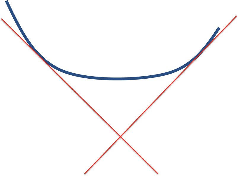
Two supporting hyperplanes of a convex function
 be the function defined by
 is the x value at which the derivative of F is p. For example, if F(x) = (x − 1)2, then
  . Note that x is a point and
  is a function. Having defined the function
  , we can write
  , which is the value of F at the point
  . Finally, the Legendre transform of F is the function
  defined by
 with slope p. To see this algebraically, consider the equation (y − y
0) = m(x − x
0) describing a line with slope m through the point (x
0, y
0). The y-intercept of this line is y
0 − mx
0. Choosing m = p and
with slope p. To see this algebraically, consider the equation (y − y
0) = m(x − x
0) describing a line with slope m through the point (x
0, y
0). The y-intercept of this line is y
0 − mx
0. Choosing m = p and  , the y-intercept is
  , which by (23.10) is − G(p).
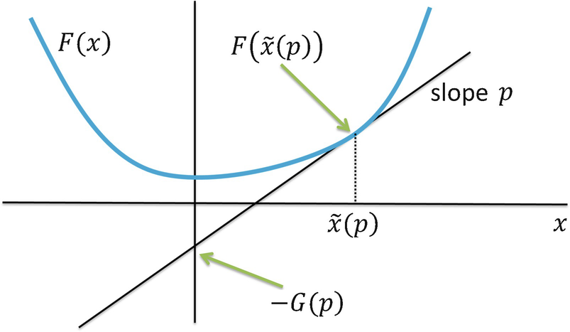
The Legendre transform G of F
Example 23.1 Consider the function F defined by F(x) = x
6. We have F
′(x) = 6x
5. Setting 6x
5 = p yields  . From (23.10) we have G(p) = p(p∕6)1∕5 − [(p∕6)1∕5]6 = [6−1∕5 − 6−6∕5]p
6∕5. □
. From (23.10) we have G(p) = p(p∕6)1∕5 − [(p∕6)1∕5]6 = [6−1∕5 − 6−6∕5]p
6∕5. □
Exercise 23.2 Derive an expression for the Legendre transform of 1 + x 4, and plot G(p) versus p. □
Exercise 23.3 Let G be the Legendre transform of F. Prove that the Legendre transform of G is F itself. □
Suppose F satisfies, in addition to assumptions (i) and (ii) above, the additional assumptions that F(x) →∞ as |x|→∞, and that F
′(x) = 0 at some point x. Then the following informal argument suggests that G is convex. Under these additional assumptions, if x ≪ 0, then p = F
′(x) ≪ 0, so the intercept − G(p) ≪ 0, which means G(p) ≫ 0. As x increases then p = F
′(x) increases, so the intercept − G(p) increases, which means G(p) decreases. As x increases beyond the point where F
′(x) = 0, the derivative p = F
′(x) continues to increase, so the intercept − G(p) decreases, which means G(p) increases. The assumptions in the above informal argument are stronger than required: it was shown in [Rockafellar 74] that if  is a finite and differentiable convex function such that for each
  the equation ∇F(x) = p has a unique solution
  , then G is a finite and differentiable convex function.
 of F, defined in [Rockafellar 74]:
 . The definition of F
⋆ does not require F to be differentiable. However, since in this section we do assume that F is twice differentiable, to maximize px − F(x) we take the derivative with respect to x and equate the derivative to 0. The maximum is achieved at the point x at which F
′(x) = p; this point is, by definition,
. The definition of F
⋆ does not require F to be differentiable. However, since in this section we do assume that F is twice differentiable, to maximize px − F(x) we take the derivative with respect to x and equate the derivative to 0. The maximum is achieved at the point x at which F
′(x) = p; this point is, by definition,  . Since F is strictly convex, then
  is the unique point yielding a global maximum, over
  , of the concave function px − F(x). This is illustrated in Fig. 23.6, where
  (the length of the green vertical bar) exceeds
  (the length of the red vertical bar), where
  is an arbitrary point not equal to
  . From (23.11) we have
  , which agrees with (23.10), since G is a special case of F
⋆. Thus G(p) = F
⋆(p).
, which agrees with (23.10), since G is a special case of F
⋆. Thus G(p) = F
⋆(p).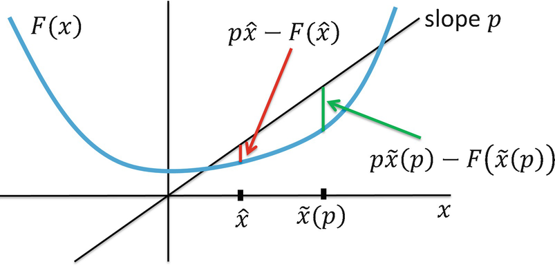
The conjugate F ⋆ of F
We have shown that, under assumptions (i) and (ii) on the convex function F, we can describe F in two different ways. The usual way is to specify the functional form of F. The Legendre transform provides a second way by specifying, for each possible value of F ′(x), the vertical intercept of the line tangent to F with slope F ′(x). While the above discussion considered only a function of a single variable, the theory of Legendre transforms and conjugate functions holds for multivariate functions [Rockafellar 74, Zia 09].
23.6 Graph Spectra
The spectrum
of  is the set of eigenvectors and eigenvalues
of the node-node adjacency matrix M
of
is the set of eigenvectors and eigenvalues
of the node-node adjacency matrix M
of  (Sect. 2.1). Since
  is undirected and has no self-loops, then the diagonal elements of M are zero, and M is symmetric (M
ij = M
ji).3 There is a large body of work, including several books, on graph spectra. To motivate our brief discussion of this subject, we consider the 1-dimensional quadratic assignment
problem studied in [Hall 70]. This is the problem of placing the nodes of
is undirected and has no self-loops, then the diagonal elements of M are zero, and M is symmetric (M
ij = M
ji).3 There is a large body of work, including several books, on graph spectra. To motivate our brief discussion of this subject, we consider the 1-dimensional quadratic assignment
problem studied in [Hall 70]. This is the problem of placing the nodes of  on a line to minimize the sum of the squared distances between adjacent nodes. (Here “adjacent” refers to adjacency in
  .) A single constraint is imposed to render infeasible the trivial solution in which all nodes are placed at the same point. Hall’s algorithm uses the method of Lagrange multipliers
for constrained optimization problems, and Hall’s algorithm can be extended to the placement of the nodes of
.) A single constraint is imposed to render infeasible the trivial solution in which all nodes are placed at the same point. Hall’s algorithm uses the method of Lagrange multipliers
for constrained optimization problems, and Hall’s algorithm can be extended to the placement of the nodes of  in two dimensions. Thus spectral graph analysis is a key technique in various methods for drawing graphs. Spectral methods are also used for community detection
in networks, particularly in social networks.
in two dimensions. Thus spectral graph analysis is a key technique in various methods for drawing graphs. Spectral methods are also used for community detection
in networks, particularly in social networks.

 . This constraint is compactly expressed as x
′x = 1. Thus the problem is to place N nodes on the line (hence the adjective 1-dimensional) to minimize the sum of squared distances, where the sum is over all pairs of adjacent nodes (i.e., adjacent in
. This constraint is compactly expressed as x
′x = 1. Thus the problem is to place N nodes on the line (hence the adjective 1-dimensional) to minimize the sum of squared distances, where the sum is over all pairs of adjacent nodes (i.e., adjacent in  ). For example, let N = 3 and let
  be the complete graph K
3. Suppose the three nodes are placed at positions 1∕6, 1∕3, and 1∕2. Since each off-diagonal element of M
ij is 1, the objective function value is
be the complete graph K
3. Suppose the three nodes are placed at positions 1∕6, 1∕3, and 1∕2. Since each off-diagonal element of M
ij is 1, the objective function value is ![$$\displaystyle \begin{aligned} \left( \frac{1}{2} \right) \left[2 \left(\frac{1}{6}-\frac{1}{3} \right)^2 + 2 \left(\frac{1}{6}-\frac{1}{2} \right )^2 + 2 \left(\frac{1}{3}-\frac{1}{2} \right)^2 \right] \, . \end{aligned}$$](../images/487758_1_En_23_Chapter/487758_1_En_23_Chapter_TeX_Equj.png)
 solves the optimization problem of minimizing (23.12) subject to the constraint x
′x = 1, since this x yields an objective function value of 0. Since this x places each node at the same position, we exclude this x and seek a non-trivial solution.
solves the optimization problem of minimizing (23.12) subject to the constraint x
′x = 1, since this x yields an objective function value of 0. Since this x places each node at the same position, we exclude this x and seek a non-trivial solution.Let D be the N × N diagonal matrix defined by  for i = 1, 2, …, N and D
ij = 0 for i ≠ j. Thus D
ii is the sum of the elements in row i of M. Since M is symmetric, D
ii is also the sum of the elements in column i of M. Compute the N × N matrix D − M, where (D − M)ij = D
ij − M
ij.
for i = 1, 2, …, N and D
ij = 0 for i ≠ j. Thus D
ii is the sum of the elements in row i of M. Since M is symmetric, D
ii is also the sum of the elements in column i of M. Compute the N × N matrix D − M, where (D − M)ij = D
ij − M
ij.
 illustrated in Fig. 23.7. Suppose columns 1, 2, 3, and 4 of M correspond to nodes a, b, c, and d, respectively. Then
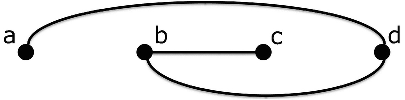
Small network to illustrate Hall’s method
 and ∑j to denote
  . We have
Let ϕ
0 be the N-dimensional column vector each of whose components is 1. The transpose ϕ
0
′ of ϕ
0 is the N-dimensional row vector (1, 1, …, 1). By definition of D we have ϕ
0
′(D − M) = 0, where the “0” on the right-hand side of this equality is the N-dimension row vector each of whose components is the number zero. Hence ϕ
0 is an eigenvector of D − M with associated eigenvalue 0. It was proved in [Hall 70] that for a connected graph  the matrix D − M has rank N − 1, which implies that the other N − 1 eigenvalues of D − M are positive.


 , placing node a to the left of node d, node d to the left of node b, and node b to the left of node c. □
 Eigenvalues and eigenvectors for the example
Eigenvalue | Eigenvector |
λ 1 = 0.0 | ϕ 1 = (0.5, 0.5, 0.5, 0.5) |
λ 2 = 0.586 | ϕ 2 = (−0.653, 0.270, 0.653, − 0.270) |
λ 3 = 2.0 | ϕ 3 = (−0.5, 0.5, − 0.5, 0.5) |
λ 4 = 3.414 | ϕ 4 = (0.270, 0.653, − 0.270, − 0.653) |
Exercise 23.4 Apply Hall’s method to find the optimal 1-dimensional layout of  when
when  is the network of three nodes connected in a ring. □
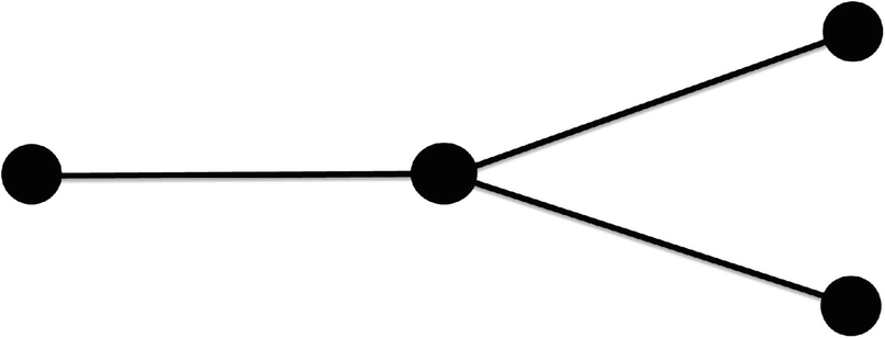
Small hub and spoke network