Scientific research involves going beyond the well-trodden and well-tested ideas and theories that form the core of scientific knowledge. During the time scientists are working things out, some results will be right, and others will be wrong. Over time, the right results will emerge.
Lisa Randall (1962- ), American, theoretical physicist, professor at Harvard University, author of “Higgs Discovery: The Power of Empty Space” (2012)
The progression of topics in this book has been to first present a fractal dimension for a geometric object  , and then to show how the same dimension can be defined for a network
  . Using this pattern, we defined, for example, the box counting dimension d
B of Ω and then of
. Using this pattern, we defined, for example, the box counting dimension d
B of Ω and then of  , the correlation dimension d
C of Ω and then of
, the correlation dimension d
C of Ω and then of  , and the information dimension d
I of Ω and then of
, and the information dimension d
I of Ω and then of  . In this chapter we continue this pattern for two additional dimensions. First, the Hausdorff dimension d
H of Ω was defined in Sect. 5.1, and in this chapter we define d
H of
. In this chapter we continue this pattern for two additional dimensions. First, the Hausdorff dimension d
H of Ω was defined in Sect. 5.1, and in this chapter we define d
H of  . Second, the family
  of generalized dimensions of Ω was defined in Sect. 16.9, and and in this chapter we define the generalized dimensions
  of
of  . The definition of d
H of
. The definition of d
H of  , and the definition of
  of
of  , were introduced in [Rosenberg 18b].
18.1 Defining the Hausdorff Dimension of a Network
Computing the box counting dimension d
B of a network  requires covering
  by a minimal set
  of boxes of diameter
at most s, for a range of values of s. Then d
B is typically computed from the slope of the
of boxes of diameter
at most s, for a range of values of s. Then d
B is typically computed from the slope of the  versus
  curve. Although, for a given s, the boxes in
  do not in general have the same diameter or mass,
this information is ignored in the computation of d
B. However, the diameters of the boxes in
do not in general have the same diameter or mass,
this information is ignored in the computation of d
B. However, the diameters of the boxes in  can be used to define the Hausdorff dimension d
H of
can be used to define the Hausdorff dimension d
H of  . The reason for studying d
H of
. The reason for studying d
H of  is that, for a geometric object, the Hausdorff dimension d
H generalizes the box counting dimension d
B, and d
H is better behaved than d
B. Thus it is of great interest to define and study d
H of
is that, for a geometric object, the Hausdorff dimension d
H generalizes the box counting dimension d
B, and d
H is better behaved than d
B. Thus it is of great interest to define and study d
H of  .
.
 , first consider computing d
B of a geometric object Ω. Recall that B(s) is the minimal number of boxes of linear size at most s required to cover Ω and that, as discussed in Sect. 4.2, we can assume that, for each given s, all boxes in the minimal covering of Ω have the same diameter. From definitions (5.1) and (5.2), if each box has diameter s, then
, first consider computing d
B of a geometric object Ω. Recall that B(s) is the minimal number of boxes of linear size at most s required to cover Ω and that, as discussed in Sect. 4.2, we can assume that, for each given s, all boxes in the minimal covering of Ω have the same diameter. From definitions (5.1) and (5.2), if each box has diameter s, then 

 . We thus treat (18.1) as an approximation, rather than as an equality.
 . For integer s, where 2 ≤ s ≤ Δ, consider a minimal s-covering
  of
of  . By Definition 7.5, the box counting dimension d
B of
. By Definition 7.5, the box counting dimension d
B of  satisfies, over some range of s and for some constant c,
 has box counting dimension d
B if, over some range of s and for some constant c,
has box counting dimension d
B if, over some range of s and for some constant c, 
Exercise 18.1 When using linear regression to estimate d
B from a range of  values, do both of the approximations (18.2) and (18.3), when treated as an equality, yield the same value of d
B? □
values, do both of the approximations (18.2) and (18.3), when treated as an equality, yield the same value of d
B? □
 has box counting dimension d
B then for some constant c such that 0 < c < ∞ we have, over some range of s,
has box counting dimension d
B then for some constant c such that 0 < c < ∞ we have, over some range of s, ![$$\displaystyle \begin{aligned} \begin{array}{rcl} B(s) [s/(\varDelta+1)]^{d_{{B}}} \approx c \, . {} \end{array} \end{aligned} $$](../images/487758_1_En_18_Chapter/487758_1_En_18_Chapter_TeX_Equ4.png)
 and the following approach to defining the Hausdorff dimension d
H of
and the following approach to defining the Hausdorff dimension d
H of  .
. let Δ
j be the diameter of box B
j,
and define
let Δ
j be the diameter of box B
j,
and define 

 is independent of the mass
of (i.e., number of nodes in) each box. We can regard
is independent of the mass
of (i.e., number of nodes in) each box. We can regard  as the “d-dimensional Hausdorff measure of
  for box size s”.
Just as d
B is that value of d for which (18.4) holds for some c and some range of s, we can view d
H as the value of d for which
for box size s”.
Just as d
B is that value of d for which (18.4) holds for some c and some range of s, we can view d
H as the value of d for which 
 are nearly equal over some range of s. Note that, since
  is not an explicit function of s, relation (18.7) does not yield a “traditional” fractal scaling law, similar to (1.1), that relates s to some appropriately defined “bulk”.
We can now justify why we replaced the approximation (18.2) with (18.3) in the definition of d
B. We want each term in the sum (18.6) to depend on d, so we want 0 < δ
j < 1 for each j. Since a box in  containing only a single node has diameter 0, adding 1 to Δ
j in (18.5) ensures that δ
j > 0 for each j. On the other hand, if a box in
containing only a single node has diameter 0, adding 1 to Δ
j in (18.5) ensures that δ
j > 0 for each j. On the other hand, if a box in  has diameter s − 1, then adding 1 to Δ in (18.5) ensures that δ
j < 1 for each j.
has diameter s − 1, then adding 1 to Δ in (18.5) ensures that δ
j < 1 for each j.
Before we formalize the definition of d
H, we must deal with non-uniqueness of  . For each s there are, in general, multiple minimal coverings
  of
of  , all yielding the same minimal value B(s). As discussed in Sect. 17.1, a definition of D
q of
, all yielding the same minimal value B(s). As discussed in Sect. 17.1, a definition of D
q of  based on the partition function
 ![$$Z_q(s) \equiv \sum _{B_{{j}} \in {\mathcal {B}}(s)} [p_{{j}}(s)]^q$$](../images/487758_1_En_18_Chapter/487758_1_En_18_Chapter_TeX_IEq51.png) can be ambiguous, since different minimal s-coverings can yield different values of Z
q(s), and hence different values of D
q. The ambiguity was resolved by requiring each minimal s-covering used to compute Z
q(s) to be lexicographically minimal. Similarly, as shown by Example 18.1 below, definition (18.6) does not in general unambiguously define
can be ambiguous, since different minimal s-coverings can yield different values of Z
q(s), and hence different values of D
q. The ambiguity was resolved by requiring each minimal s-covering used to compute Z
q(s) to be lexicographically minimal. Similarly, as shown by Example 18.1 below, definition (18.6) does not in general unambiguously define  , since different minimal s-coverings can yield different values of
  .
.


 for d > 1, with equality when d = 1. □
Two minimal 3-coverings of a 7 node chain
 can be eliminated by adapting the lexicographic approach of [Rosenberg 17b], described in Sect. 17.1. Consider a minimal s-covering
  and define J ≡ B(s). Recalling that Δ
j is the diameter of box
and define J ≡ B(s). Recalling that Δ
j is the diameter of box  , we associate with
  the point
 . An unambiguous choice of a minimal s-covering is to pick the minimal s-covering for which the associated diameter vector is lexicographically smallest.
That is, suppose that, for a given s, there are two distinct minimal s-coverings
. An unambiguous choice of a minimal s-covering is to pick the minimal s-covering for which the associated diameter vector is lexicographically smallest.
That is, suppose that, for a given s, there are two distinct minimal s-coverings  and
and  . Let
. Let  be the diameter vector associated with
  , and let
  be the diameter vector associated with
  . Then we choose
  if
if  , where “≽” denotes lexicographic ordering. Applying this to the two minimal 3-coverings of Fig. 18.1, the associated diameter vectors are (2, 2, 0) for (i) and (2, 1, 1) for (ii). Since (2, 2, 0) ≽ (2, 1, 1) we choose the covering (ii).
 , we can now formalize the definition of d
H of
, we can now formalize the definition of d
H of  as that value of d for which
  is roughly constant over a range of s. Let
  be a given set of integer values of s such that 2 ≤ s ≤ Δ for
  . For example, for integers L, U such that 2 ≤ L < U ≤ Δ we might set
  . For a given d > 0, define
  to be the standard deviation (in the usual statistical sense) of the values
  for
for  as follows. Define
 as the “average d-dimensional Hausdorff measure of
  for box sizes in
  ”. Next we compute the standard deviation of the Hausdorff measures:
 ![$$\displaystyle \begin{aligned} \begin{array}{rcl} \sigma({\mathbb{G}},{\mathcal{S}},d) &\displaystyle \equiv &\displaystyle \sqrt { \frac{1}{\vert {\mathcal{S}} \vert} \sum_{s \in {\mathcal{S}}} \big[ \, m({\mathbb{G}}, s, d) - m_{\textit{avg}}({\mathbb{G}}, {\mathcal{S}}, d) \, \big]^2 } \; . {} \end{array} \end{aligned} $$](../images/487758_1_En_18_Chapter/487758_1_En_18_Chapter_TeX_Equ9.png)
 the Hausdorff dimension d
H, defined as follows.
the Hausdorff dimension d
H, defined as follows.
Definition 18.2 [Rosenberg 18b] (Part A.) If  has at least one local minimum over {d | d > 0}, then d
H is the value of d satisfying (i)
has at least one local minimum over {d | d > 0}, then d
H is the value of d satisfying (i)  has a local minimum at d
H, and (ii) if
has a local minimum at d
H, and (ii) if  has another local minimum at
  , then
  . (Part B.) If
  does not have a local minimum over {d | d > 0}, then d
H ≡∞. □
does not have a local minimum over {d | d > 0}, then d
H ≡∞. □
For all of the networks studied in [Rosenberg 18b], d H is finite. An interesting open question is whether there exists a network with a finite d B and infinite d H.
Definition 18.3 [Rosenberg 18b] If d
H < ∞, then the Hausdorff measure of  is
is  . If d
H = ∞, then the Hausdorff measure of
. If d
H = ∞, then the Hausdorff measure of  is 0. □
 . For a given
  , choosing different
  will in general yield different values of d
H; this is not surprising, and a similar dependence was studied in Sect. 17.2. The reason, in Part A of Definition 18.2, for requiring d
H to yield a local minimum of
will in general yield different values of d
H; this is not surprising, and a similar dependence was studied in Sect. 17.2. The reason, in Part A of Definition 18.2, for requiring d
H to yield a local minimum of  is that by definitions (18.5) and (18.6) for each s we have
 . From (18.10), we know that
  is not a convex function of d. Thus the possibility exists that
  might have multiple local minima. To deal with that possibility, we require that
  be smaller than the standard deviation at any other local minimum. As for Part B, it may be possible that
  has no local minimum. In this case, by virtue of (18.10) we define d
H = ∞.
has no local minimum. In this case, by virtue of (18.10) we define d
H = ∞.By Definition 18.2, the computation of d
H of  requires a line search (i.e., a 1-dimensional minimization) to minimize
  over d > 0.
Since
over d > 0.
Since  might have multiple local minima, we cannot use line search methods such as bisection or golden search [Wilde 64] designed for minimizing a unimodal function. Instead, in [Rosenberg 18b] d
H was computed by evaluating
might have multiple local minima, we cannot use line search methods such as bisection or golden search [Wilde 64] designed for minimizing a unimodal function. Instead, in [Rosenberg 18b] d
H was computed by evaluating  from d = 0.1 to d = 6, in increments of 10−4, and testing for a local minimum (this computation took at most a few seconds on a laptop). For all of the networks studied,
  had exactly one local minimum. While these computational results do not preclude the possibility of multiple local minima for some other network, a convenient working definition is that d
H is the value of d yielding a local minimum of the standard deviation
had exactly one local minimum. While these computational results do not preclude the possibility of multiple local minima for some other network, a convenient working definition is that d
H is the value of d yielding a local minimum of the standard deviation  .
.
In scientific applications of fractal analysis, it is well-established that the ability to calculate a fractal dimension of a geometric object does not convey information about the structure of the object. For example, box counting was used in [Karperien 13] to calculate d B of microglia (a type of cell occurring in the central nervous system of invertebrates and vertebrates). However, we were warned in [Karperien 13] that the fractal dimension of an object “does not tell us anything about what the underlying structure looks like, how it was constructed, or how it functions”. Moreover, the ability to calculate a fractal dimension of an object “does not mean the phenomenon from which it was gleaned is fractal; neither does a phenomenon have to be fractal to be investigated with box counting fractal analysis”.
Similarly, the ability to calculate d
H of  does not provide any information about the structure of
  . Indeed, for a network
  the definitions of fractality and self-similarity are quite different [Gallos 07b]; as discussed in Sect. 7.2, the network
  is fractal if
  for a finite exponent d
B, while
for a finite exponent d
B, while  is self-similar if the node degree
distribution of
is self-similar if the node degree
distribution of  remains invariant over several generations of renormalization.
(Renormalizing
remains invariant over several generations of renormalization.
(Renormalizing  , as discussed in Chap. 21, means computing an s-covering of
  , merging all nodes in each box in the s-covering into a supernode, and connecting two supernodes if the corresponding boxes are connected by one or more arcs in the original network.)
Moreover, “Surprisingly, this self-similarity under different length scales seems to be a more general feature that also applies in non-fractal networks such as the Internet. Although the traditional fractal theory does not distinguish between fractality and self-similarity, in networks these two properties can be considered to be distinct” [Gallos 07b]. With this caveat on the interpretation of a fractal dimension of
, merging all nodes in each box in the s-covering into a supernode, and connecting two supernodes if the corresponding boxes are connected by one or more arcs in the original network.)
Moreover, “Surprisingly, this self-similarity under different length scales seems to be a more general feature that also applies in non-fractal networks such as the Internet. Although the traditional fractal theory does not distinguish between fractality and self-similarity, in networks these two properties can be considered to be distinct” [Gallos 07b]. With this caveat on the interpretation of a fractal dimension of  , in the next section we compute d
H of several networks.
, in the next section we compute d
H of several networks.
18.2 Computing the Hausdorff Dimension of a Network
The following examples from [Rosenberg 18b] illustrate the computation of d
H of some networks, ranging from a small constructed example of 5 nodes to a real-world protein network of 1458 nodes. Since fractality and self-similarity of  are distinct characteristics, d
H can be meaningfully computed even for small networks without any regular or self-similar structure.
are distinct characteristics, d
H can be meaningfully computed even for small networks without any regular or self-similar structure.
 . For s = 2 the three boxes in
  have diameter 1, and 1, and 0, so from definitions (18.5) and (18.6) we have
  . For s = 3 the two boxes in
  have diameter 2 and 1, so
  . Figure 18.2 (right) plots
  and
and  versus d. Set
  . Since for d = 1 we have
  , then d
H = 1 and
, then d
H = 1 and  . Moreover, d
H = 1 is the unique point minimizing
. Moreover, d
H = 1 is the unique point minimizing  . For this network we have d
H = d
B. By Definition 18.3, the Hausdorff measure
. For this network we have d
H = d
B. By Definition 18.3, the Hausdorff measure  of
of  is 5∕4. □
chair network (left) and d H calculation (right)
 has Δ = 4; the bottom network
  has Δ = 5. Figure 18.4 shows box counting results, for s = 2 and s = 3, for the two networks. For s = 2 we have, for both networks, B(2) = 4, B(3) = 2, and B(4) = 2. Since B(3) = B(4), to compute d
B we ignore the s = 4 results and choose
has Δ = 5. Figure 18.4 shows box counting results, for s = 2 and s = 3, for the two networks. For s = 2 we have, for both networks, B(2) = 4, B(3) = 2, and B(4) = 2. Since B(3) = B(4), to compute d
B we ignore the s = 4 results and choose  . This yields, for both networks,
  .
.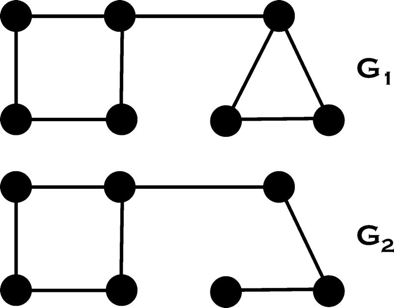
Two 7 node networks with the same d B but different d H
Box counting results for s = 2 (left) and s = 3 (right)
For  , from (18.5) and (18.6) we have
  and
and  . For
. For  , the plots of
  versus d and
  versus d intersect at d
H = 2, and
versus d intersect at d
H = 2, and  . Hence
  , and d
H = 2 is the unique point minimizing
, and d
H = 2 is the unique point minimizing  . Thus for
  and
and  we have d
H = 2 > 1.71 ≈ d
B, so the inequality d
H ≤ d
B, known to hold for a geometric object [Falconer 03], can fail to hold for a network. By Definition 18.3, the Hausdorff measure
we have d
H = 2 > 1.71 ≈ d
B, so the inequality d
H ≤ d
B, known to hold for a geometric object [Falconer 03], can fail to hold for a network. By Definition 18.3, the Hausdorff measure  of
of  is 13∕25.
Turning now to  , from (18.5) and (18.6) we have
  and
and  . The plots of
  versus d and and
  versus d intersect at d
H ≈ 1.31, and
versus d intersect at d
H ≈ 1.31, and  . Thus for
  and
and  we have
  , and
, and  . The two networks
  and
and  in Example 18.3 have the same number of nodes and the same d
B, yet have different d
H. □
in Example 18.3 have the same number of nodes and the same d
B, yet have different d
H. □
Example 18.3 suggests that d
H can be better than d
B for comparing two networks, or for studying the evolution of a network over time. The reason d
H provides a “finer” measure than d
B is that d
B considers only the variation in the number B(s) of boxes needed to cover the network, while d
H recognizes that the different boxes in the covering  will in general have different diameters.
The next two examples, from [Rosenberg 18b], show that the Hausdorff dimension of
will in general have different diameters.
The next two examples, from [Rosenberg 18b], show that the Hausdorff dimension of  produces expected “classical” results: for a large 1-dimensional chain we have d
H = 1, and for a large 2-dimensional rectilinear grid we have d
H = 2.
produces expected “classical” results: for a large 1-dimensional chain we have d
H = 1, and for a large 2-dimensional rectilinear grid we have d
H = 2.
 be a chain of N nodes, so Δ = N − 1. For s ≪ N, an s-covering of
  consists of ⌊N∕s⌋ boxes, each containing s nodes and having diameter s − 1, and one box containing N − s⌊N∕s⌋ nodes and having diameter N − s⌊N∕s⌋− 1. By definitions (18.5) and (18.6), for s ≪ N we have
 . Now let
  be a (finite) set of box sizes, such that s ≪ N for
  . By definitions (18.8) and (18.9), setting d = 1 yields
  , so d
H = 1 for a long chain of N nodes. □
, so d
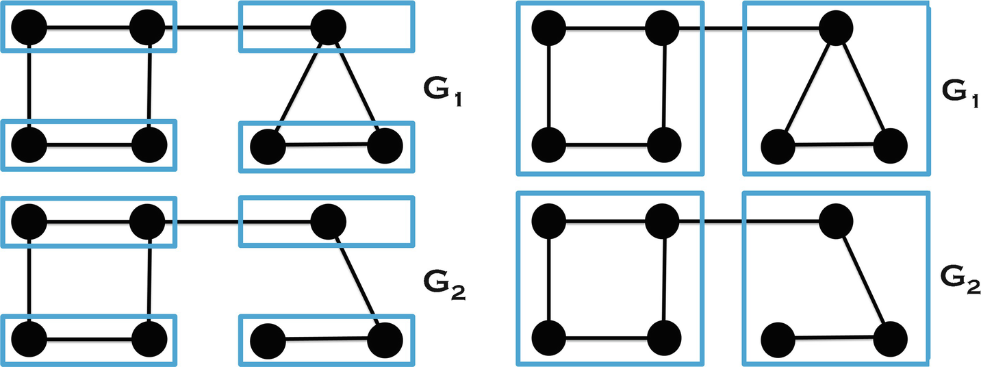
H = 1 for a long chain of N nodes. □ nodes within distance r of node z; the box containing these n(r) nodes has diameter 2r, and the box size s for this box is given by s = 2r + 1. Now consider a finite version of the infinite two-dimensional rectilinear lattice, defined as follows. For a positive integer K ≫ 1, let
  be a K × K two-dimensional rectilinear lattice such that each node has integer coordinates, where node (i, j) is adjacent to (i − 1, j), (i + 1, j), (i, j − 1), and (i, j + 1), and where each edge of the lattice contains K nodes. The diameter Δ of
  is 2(K − 1). Figure 18.5 illustrates a box of radius r = 1 in the “interior” of a 6 × 6 lattice.
Box of radius r = 1 in a 6 × 6 rectilinear grid
 using boxes of radius r consists of approximately K
2∕n(r) “totally full” boxes with n(r) nodes and diameter 2r, and
using boxes of radius r consists of approximately K
2∕n(r) “totally full” boxes with n(r) nodes and diameter 2r, and  “partially full” boxes of diameter not exceeding 2r and containing fewer than n(r) nodes; these
  partially full boxes are needed around the 4 edges of
  . Since K ≫ 1, we ignore these
  partially full boxes, and
Setting d = 2 yields  , so d
H = 2 for a large K × K rectilinear lattice. □
, so d
H = 2 for a large K × K rectilinear lattice. □
 , Fig. 18.6 shows that the
  versus
  curve is approximately linear for
  . (In this example, as well as in subsequent examples, the determination of the set
  was done by visual inspection.) Linear regression over this range yields d
B ≈ 2.38. As discussed in Sect. 18.1, d
B can also be viewed as the value of d minimizing, over {d | d > 0}, the standard deviation of the terms B(s)[s∕(Δ + 1)]d for
was done by visual inspection.) Linear regression over this range yields d
B ≈ 2.38. As discussed in Sect. 18.1, d
B can also be viewed as the value of d minimizing, over {d | d > 0}, the standard deviation of the terms B(s)[s∕(Δ + 1)]d for  . Figure 18.7 (left) plots B(s)[s∕(Δ + 1)]d versus d for
  for the dolphins network. The standard deviation is minimized at d ≈ 2.41, which is very close to d
B ≈ 2.38.
for the dolphins network. The standard deviation is minimized at d ≈ 2.41, which is very close to d
B ≈ 2.38.
 versus
  for the dolphins network

B(s)[s∕(Δ + 1)]d versus d for  (left) and
  versus d (right) for dolphins
 was used to calculate d
H of the dolphins network. Figure 18.7 (right) plots
was used to calculate d
H of the dolphins network. Figure 18.7 (right) plots  for
for  over the range d ∈ [1.6, 3]. Figure 18.8 (left), which plots
  versus d over the range d ∈ [0, 3], shows that the location of d
H is not immediately evident. Numerical calculation revealed that
versus d over the range d ∈ [0, 3], shows that the location of d
H is not immediately evident. Numerical calculation revealed that  has a unique local minimum at d
H ≈ 2.34. Figure 18.8 (right) shows that
has a unique local minimum at d
H ≈ 2.34. Figure 18.8 (right) shows that  is quite “flat”1 in the vicinity of d
H, since for d ∈ [2.26, 2.40] we have
is quite “flat”1 in the vicinity of d
H, since for d ∈ [2.26, 2.40] we have  . □
. □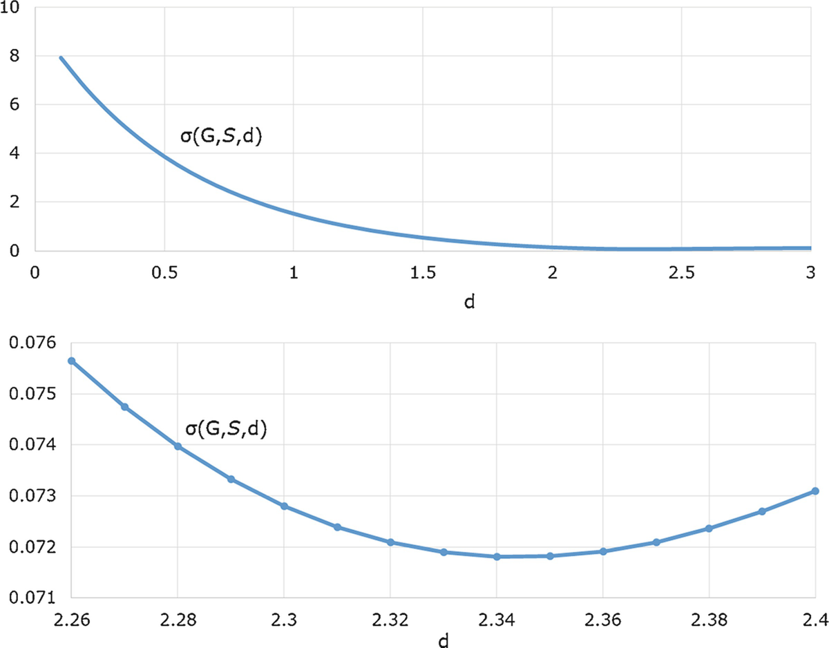
 versus d for dolphins for d ∈ [0, 3] (left) and d ∈ [2.26, 2.40] (right)
 , linear regression over this range yields d
B ≈ 4.04. The shape of the
, linear regression over this range yields d
B ≈ 4.04. The shape of the  versus d plot for this network closely resembles the shape in Fig. 18.8 (left). There is a unique local minimum of
  at d
H ≈ 4.02. The standard deviation
at d
H ≈ 4.02. The standard deviation  is also quite flat in the vicinity of d
H. □
is also quite flat in the vicinity of d
H. □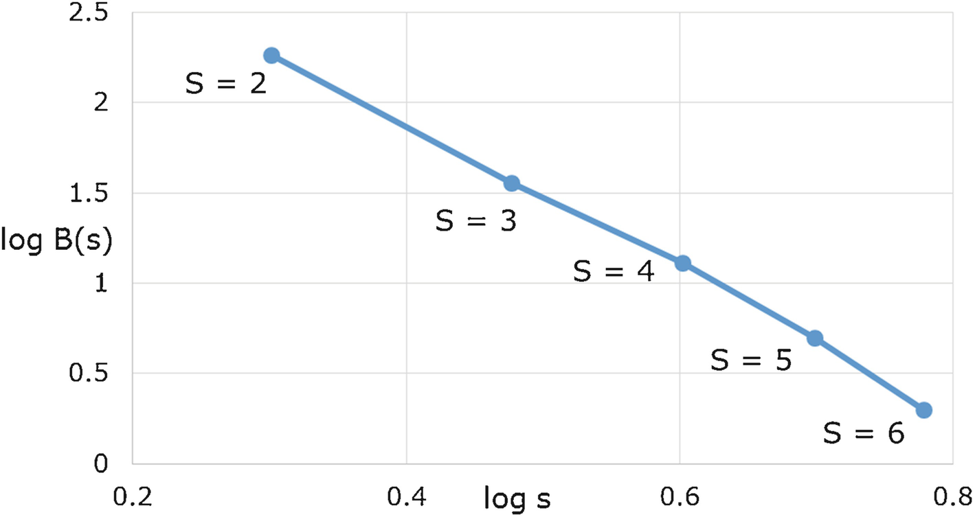
 versus
  for the USAir97 network
 , linear regression over this range yields d
B ≈ 2.66. Figure 18.10 (right) plots
, linear regression over this range yields d
B ≈ 2.66. Figure 18.10 (right) plots  for
for  over the range d ∈ [1.6, 4]. There is a unique local minimum of
  at d
H ≈ 3.26. □
at d
H ≈ 3.26. □
 versus
  (left) and
  versus d (right) for the jazz network
 , a linear fit is reasonable for the other five points, so we set
  . Linear regression over this range yields d
B ≈ 2.68. Figure 18.11 (right) plots
. Linear regression over this range yields d
B ≈ 2.68. Figure 18.11 (right) plots  for
for  over the range d ∈ [1.5, 5]. Figure 18.12 (left) plots
  versus d over the range d ∈ [0, 5]. There is a unique local minimum of
  at d
H ≈ 3.51.
at d
H ≈ 3.51.
 versus
  (left) and
  versus d (right) for the C. elegans network

 versus d for C. elegans for d ∈ [0, 5] (left) and d ∈ [2.26, 2.40] (right)
Again, the  versus d plot is very flat in the vicinity of d
H, as shown by Fig. 18.12 (right), since for d ∈ [3.45, 3.55] we have
versus d plot is very flat in the vicinity of d
H, as shown by Fig. 18.12 (right), since for d ∈ [3.45, 3.55] we have  . □
. □
 , Fig. 18.13 shows that
  is close to linear in
  for
for  (the dotted line is the linear least squares fit), and d
B = 2.44. The shape of the
(the dotted line is the linear least squares fit), and d
B = 2.44. The shape of the  versus d plot for protein has a shape similar to the plot for C. elegans, and for the protein network there is a unique local minimum of
  at d
H = 3.08. □
at d
H = 3.08. □
 versus
  for s ∈ [4, 14] for the protein network
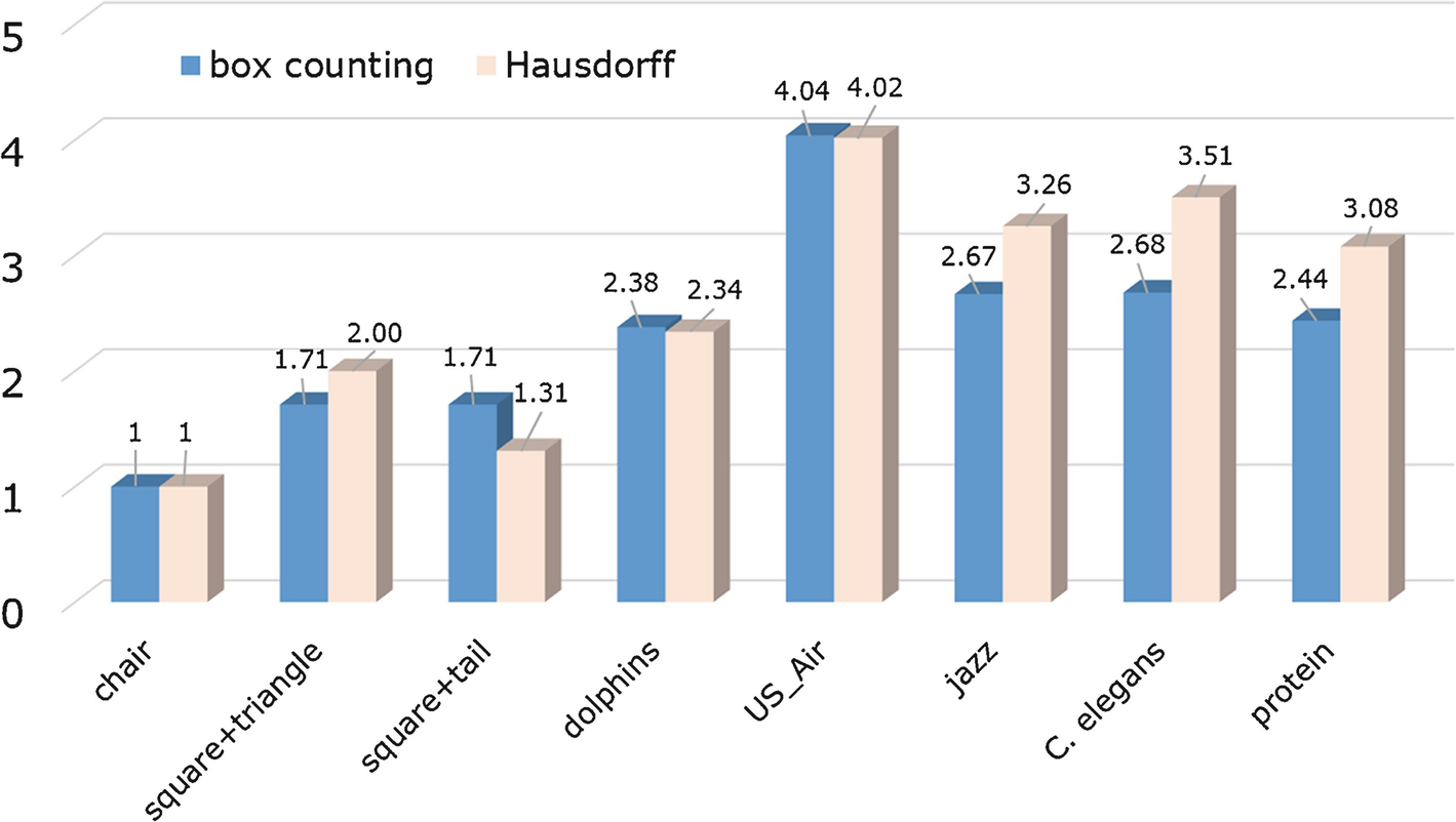
Summary of d B and d H computations
The above examples show that it is computationally feasible to compute d
H of a network. The numerical value of d
H depends not only on the minimal number B(s) of boxes for each box size s, but also on the diameters of the boxes in  . Any method for computing the box counting dimension d
B of
. Any method for computing the box counting dimension d
B of  suffers from the fact that in general we cannot verify that the computed B(s) is in fact minimal (although a lower bound on B(s) can be computed [Rosenberg 13]).
Computing the Hausdorff dimension adds the further complication that there is currently no way to verify that a lexico minimal covering (Sect. 17.1) has been found. Therefore, since for each box size s a randomized box-counting method is typically employed (e.g., the above results used the method described in [Rosenberg 17b]), it is necessary to run sufficiently many randomized iterations until we are reasonably confident that not only has a minimal covering of
suffers from the fact that in general we cannot verify that the computed B(s) is in fact minimal (although a lower bound on B(s) can be computed [Rosenberg 13]).
Computing the Hausdorff dimension adds the further complication that there is currently no way to verify that a lexico minimal covering (Sect. 17.1) has been found. Therefore, since for each box size s a randomized box-counting method is typically employed (e.g., the above results used the method described in [Rosenberg 17b]), it is necessary to run sufficiently many randomized iterations until we are reasonably confident that not only has a minimal covering of  been obtained, but also that a lexicographically minimal covering has been obtained. This extra computational burden is not unique to computing d
H, since computing any fractal dimension of
been obtained, but also that a lexicographically minimal covering has been obtained. This extra computational burden is not unique to computing d
H, since computing any fractal dimension of  other than the box counting dimension requires an unambiguous selection of a minimal covering, e.g., computing the information dimension d
I of
other than the box counting dimension requires an unambiguous selection of a minimal covering, e.g., computing the information dimension d
I of  requires finding a maximal entropy minimal covering (Sect. 15.4), and computing the generalized dimensions D
q of
requires finding a maximal entropy minimal covering (Sect. 15.4), and computing the generalized dimensions D
q of  requires finding a lexico minimal summary vector.
 . Let the arc set
  of
of  be specified by a list
  , so that
  is built, arc by arc, by processing the list
  . After each arc is processed, the node degree
δ
n of each node n in
. After each arc is processed, the node degree
δ
n of each node n in  is updated. To perturb
  , choose P ∈ (0, 1). After reading arc a from
  , pick two random probabilities p
1 ∈ (0, 1) and p
2 ∈ (0, 1). If p
1 < P, modify arc a as follows. Let i and j be the endpoints of arc a. If δ
i > 1 and
, pick two random probabilities p
1 ∈ (0, 1) and p
2 ∈ (0, 1). If p
1 < P, modify arc a as follows. Let i and j be the endpoints of arc a. If δ
i > 1 and  , replace the endpoint i of arc a with a randomly chosen node distinct from i; otherwise, if δ
j > 1, replace the endpoint j of arc a with a randomly chosen node distinct from j. (Requiring δ
i > 1 ensures i will not become an isolated node.) This perturbation method was applied to the jazz network of
Example 18.8 for P ranging from 0.01 to 0.08. The results, in Fig. 18.15, show that the d
H versus P plot has roughly the same shape as the d
B versus P plot. Although the range of d
H over the interval 0 ≤ P ≤ 0.08 is smaller than the range of d
B, sometimes d
H magnifies the effect of a perturbation, e.g., d
H changed much more than d
B when P increased from 0.02 to 0.03. □
, replace the endpoint i of arc a with a randomly chosen node distinct from i; otherwise, if δ
j > 1, replace the endpoint j of arc a with a randomly chosen node distinct from j. (Requiring δ
i > 1 ensures i will not become an isolated node.) This perturbation method was applied to the jazz network of
Example 18.8 for P ranging from 0.01 to 0.08. The results, in Fig. 18.15, show that the d
H versus P plot has roughly the same shape as the d
B versus P plot. Although the range of d
H over the interval 0 ≤ P ≤ 0.08 is smaller than the range of d
B, sometimes d
H magnifies the effect of a perturbation, e.g., d
H changed much more than d
B when P increased from 0.02 to 0.03. □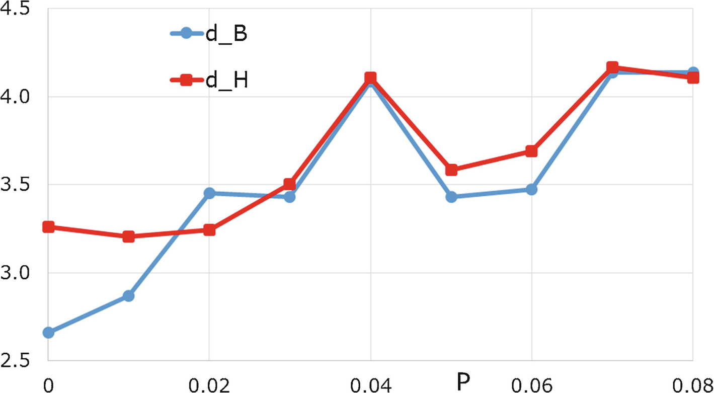
Perturbations of the jazz network

d B and d H of a network growing with preferential attachment
18.3 Generalized Hausdorff Dimensions of a Network
In Sect. 16.9 we presented the definition in [Grassberger 85] of the generalized Hausdorff dimensions  of a geometric object. Continuing our approach in this book of defining a fractal dimension for a geometric object and then extending it to a network, and having defined the Hausdorff dimension d
H of a network
of a geometric object. Continuing our approach in this book of defining a fractal dimension for a geometric object and then extending it to a network, and having defined the Hausdorff dimension d
H of a network  in Sect. 18.1 of this chapter, in this section we study the generalized Hausdorff dimensions
  of
of  , defined in [Rosenberg 18b]. These dimensions utilize both the diameter and mass of each box in the minimal covering
  of
of  . Just as the computation of d
H for
. Just as the computation of d
H for  requires a line search, for each q the computation of the generalized Hausdorff dimension
  of
of  also requires a line search.
 be a minimal s-covering of
  . The probability of box
  is, as usual, p
j(s) ≡ N
j(s)∕N, where N
j(s) is the number of nodes contained in box B
j; for simplicity we write p
j instead of p
j(s). Recalling that δ
j is defined by (18.5), we borrow from [Grassberger 85] and define
is, as usual, p
j(s) ≡ N
j(s)∕N, where N
j(s) is the number of nodes contained in box B
j; for simplicity we write p
j instead of p
j(s). Recalling that δ
j is defined by (18.5), we borrow from [Grassberger 85] and define 
 as the “d-dimensional generalized Hausdorff measure of order q of
  for box size s”.
Exercise 18.2 Prove that for q ≠ 1 the derivative with respect to d of  is negative. □
 of
of  as that value of d for which
  is roughly constant over a given range
  of values of s. For d > 0, let
  be the standard deviation of the values
  for
for  :
: ![$$\displaystyle \begin{aligned} m_{\textit{avg}}({\mathbb{G}}, {\mathcal{S}}, q, d) & \equiv \frac{1}{\vert {\mathcal{S}} \vert} \sum_{s \in {\mathcal{S}}} m({\mathbb{G}}, s, q, d) \\ \sigma({\mathbb{G}},{\mathcal{S}}, q, d) & \equiv \sqrt { \frac{1}{\vert {\mathcal{S}} \vert} \sum_{s \in {\mathcal{S}}} \big[ \, m({\mathbb{G}}, s, q, d) - m_{\textit{avg}}({\mathbb{G}}, {\mathcal{S}}, q, d) \, \big]^2. } \; \; {} \end{aligned} $$](../images/487758_1_En_18_Chapter/487758_1_En_18_Chapter_TeX_Equ12.png)
 the generalized Hausdorff dimension of order q, denoted by
  , defined as follows.
Definition 18.4 [Rosenberg 18b] (Part A.) If  has at least one local minimum over {d | d > 0}, then
  is the value of d satisfying (i)
  has a local minimum at
  , and (ii) if
  has another local minimum at
  , then
  . (Part B.) If
  does not have a local minimum over {d | d > 0}, then
  . □
. □
Definition 18.5 If  , then the generalized Hausdorff measure of order q of
  is
is  . If
. If  then the generalized Hausdorff measure of order q of
  is 0. □
Setting q = 0, by (18.6) and (18.11) we have  . By (18.9) and (18.12) we have
  . Hence, by Definitions 18.2 and 18.4 we have
  . In words, the generalized Hausdorff dimension of order 0 of
  is equal to the Hausdorff dimension of
  .
.
For a geometric object Ω, it was observed in [Grassberger 85] that if μ is the Hausdorff measure, then  for all q, at least for strictly self-similar fractals. The following theorem, the analogue of Grassberger’s observation for a network
  , says that if the mass
of each box is proportional to δ
j, then for q ≠ 1 we have
, says that if the mass
of each box is proportional to δ
j, then for q ≠ 1 we have  .
.
Theorem 18.1 [Rosenberg 18b] Suppose that for some constant α > 0 we have δ
j = αp
j for  and for
  . Then for q ≠ 1 we have
  and the generalized Hausdorff measure of order q of
  is α.
is α.
 and for
  . Set d = 1 and pick q ≠ 1. From (18.11), for
  we have
 ![$$\displaystyle \begin{aligned} \begin{array}{rcl} m({\mathbb{G}}, s, q, 1)\!\!\!\! &\displaystyle = &\displaystyle \!\!\!\! \left[ \sum_{B_{{j}} \in {\mathcal{B}}(s)} p_{{j}} \left( \frac{\delta_{{j}}}{p_{{j}}} \right)^{1-q} \right]^{1/(1-q)} \; = \;\;\; \left[ \sum_{B_{{j}} \in {\mathcal{B}}(s)} p_{{j}} \left( \frac{\alpha p_{{j}}}{ p_{{j}}} \right)^{1-q} \right]^{1/(1-q)} \\ \!\!\!\!&\displaystyle = &\displaystyle \!\!\!\! \left[ \alpha^{1-q} \sum_{B_{{j}} \in {\mathcal{B}}(s)} p_{{j}} \right]^{1/(1-q)} \; = \;\;\; \alpha \, , \end{array} \end{aligned} $$](../images/487758_1_En_18_Chapter/487758_1_En_18_Chapter_TeX_Equ13.png)
 . Since
  , by (18.12) we have
  . By Definition 18.4, we have
  . By Definition 18.5, the generalized Hausdorff measure of order q of
  is α. □
Exercise 18.3 Suppose that for some constant α > 0 we have δ
j = αp
j for  and for
  . What are the values of d
I and
. What are the values of d
I and  ? □
? □
Example 18.13 Consider again the chair network of
Example 18.2. As shown in Fig. 18.2, the box with 1 node has p
j = 1∕5 and δ
j = 1∕4, each box with 2 nodes has p
j = 2∕5 and δ
j = 2∕4, and the box with 3 nodes has p
j = 3∕5 and δ
j = 3∕4. Since the conditions of Theorem 18.1 are satisfied with α = 5∕4, for q ≠ 1 we have  , and the generalized Hausdorff measure of order q of the chair network is 5∕4. □
 of Fig. 18.3. Figure 18.17 plots
  versus q for integer q ∈ [−10, 10]. Clearly
  is not monotonic decreasing in q, even over the range q ≥ 0, since
  . Since for a geometric fractal
  is a non-increasing function of q [Grassberger 85], the non-monotonic behavior in Fig. 18.17 is perhaps surprising. However, the generalized dimensions D
q of a network, computed using Definition 17.3, also can fail to be monotone decreasing in q (Sect. 17.2). Thus it is not unexpected that the generalized Hausdorff dimensions of a network, computed using Definition 18.4, can also exhibit non-monotonic behavior. □
is a non-increasing function of q [Grassberger 85], the non-monotonic behavior in Fig. 18.17 is perhaps surprising. However, the generalized dimensions D
q of a network, computed using Definition 17.3, also can fail to be monotone decreasing in q (Sect. 17.2). Thus it is not unexpected that the generalized Hausdorff dimensions of a network, computed using Definition 18.4, can also exhibit non-monotonic behavior. □

 versus q for the network
  of Fig. 18.3
 . Figure 18.18 plots
  versus q. Remarkably, there is a “critical order” q
c ≈−1.54 such that
versus q. Remarkably, there is a “critical order” q
c ≈−1.54 such that  is finite for q > q
c and
is finite for q > q
c and  is infinite for q < q
c. □
is infinite for q < q
c. □
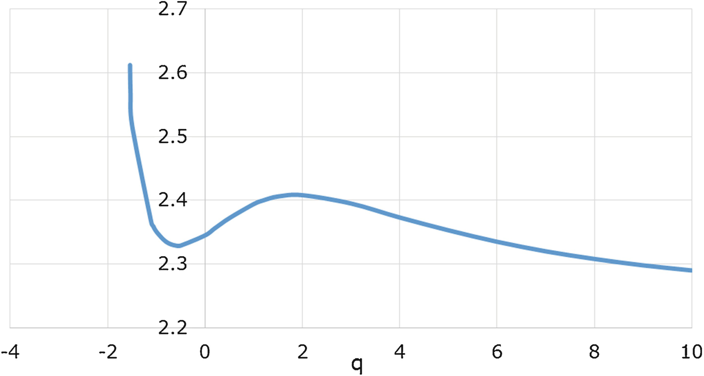
 versus q for the dolphins network
 . Figure 18.19 plots
  versus q. There is a critical interval Q
c ≈ [−3.9, −0.3] such that
versus q. There is a critical interval Q
c ≈ [−3.9, −0.3] such that  is infinite for q ∈ Q
c and finite otherwise. □
is infinite for q ∈ Q
c and finite otherwise. □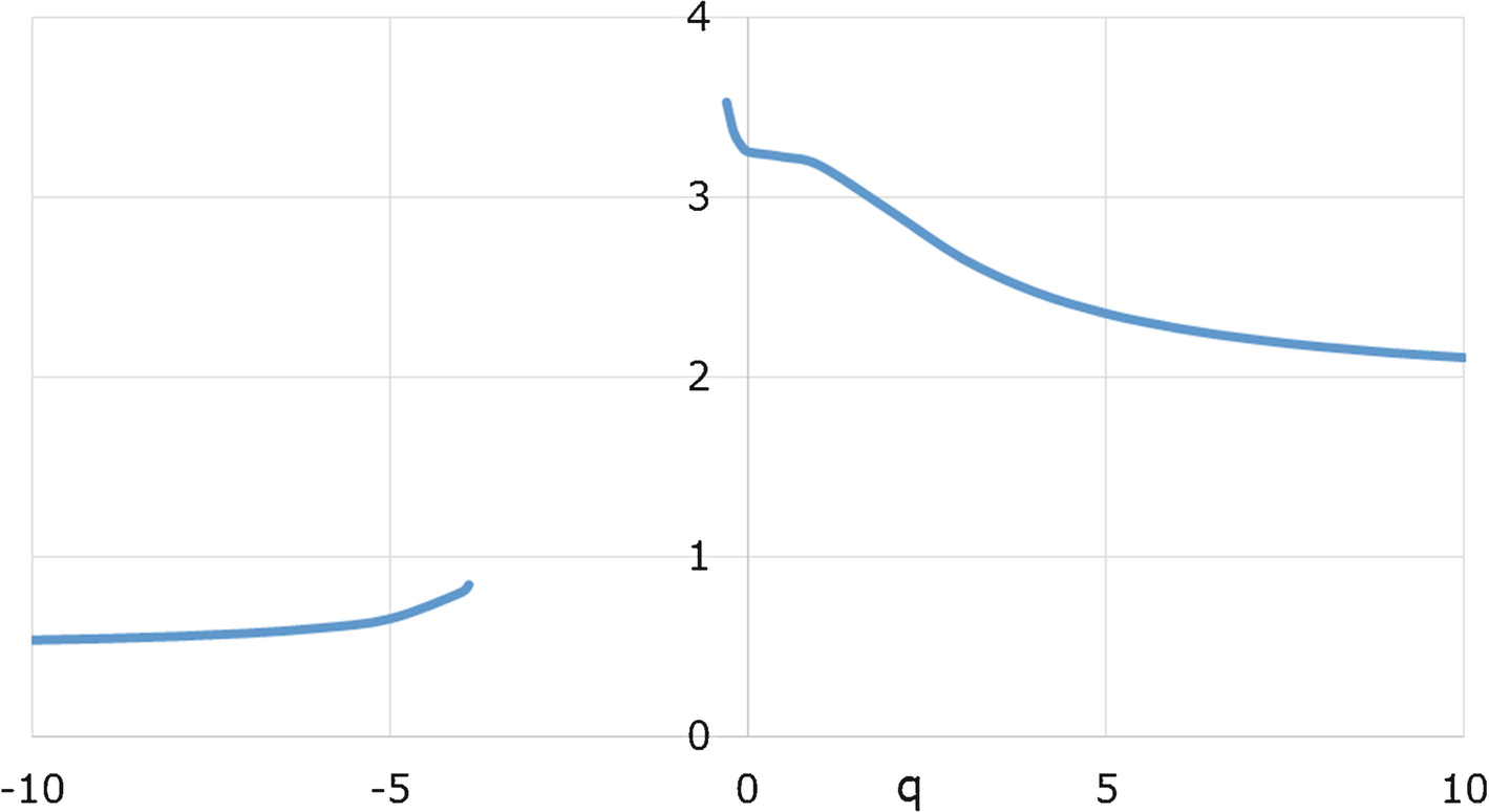
 versus q for the jazz network
 . Figure 18.20 plots
  versus q. There is a critical interval Q
c ≈ [−1.45, −0.25] such that
versus q. There is a critical interval Q
c ≈ [−1.45, −0.25] such that  is infinite for q ∈ Q
c and finite otherwise. □
is infinite for q ∈ Q
c and finite otherwise. □
 versus q for the C. elegans network
The above examples show that  can exhibit complicated behavior for q < 0. These findings align with several studies (e.g., [Block 91]) pointing to difficulties in computing and interpreting D
q for a geometric object and the difficulties “imperceptibly hidden” in the negative q domain [Riedi 95]; see Sect. 16.4. Thus, for a network,
can exhibit complicated behavior for q < 0. These findings align with several studies (e.g., [Block 91]) pointing to difficulties in computing and interpreting D
q for a geometric object and the difficulties “imperceptibly hidden” in the negative q domain [Riedi 95]; see Sect. 16.4. Thus, for a network,  should probably be computed only for q ≥ 0. The existence of a critical interval in Examples 18.15–18.17 raises many questions, e.g., to characterize the class of networks possessing a critical interval.
To summarize the computational results presented in this chapter, d
H can sometimes be more useful than d
B in quantifying changes in the topology of a network. However, d
H is harder to compute than d
B, and  is less well behaved than D
q. We conclude that d
H and
is less well behaved than D
q. We conclude that d
H and  should be added to the set of useful metrics for characterizing a network, but they cannot be expected to replace d
B and D
q.
should be added to the set of useful metrics for characterizing a network, but they cannot be expected to replace d
B and D
q.