My power flurries through the air into the ground
My soul is spiraling in frozen fractals all around
And one thought crystallizes like an icy blast
I’m never going back
The past is in the past
Lyrics from the song “Let It Go”, from the 2013 movie “Frozen”. Music and lyrics by Kristen Anderson-Lopez and Robert Lopez.
In Chap. 16 we presented the theory of generalized dimensions for a geometric object Ω, and discussed several methods for computing the generalized dimensions of Ω. In this chapter we draw upon the content of Chap. 16 to show how generalized dimensions can be defined and computed for a complex network  .
.
17.1 Lexico Minimal Coverings
In Chap. 15, we showed that the definition proposed in [Wei 14a] of the information dimension d
I of a network  is ambiguous, since d
I is computed from a minimal s-covering of
is ambiguous, since d
I is computed from a minimal s-covering of  , for a range of s, and there are in general multiple minimal s-coverings of
  , yielding different values of d
I. Using the maximal entropy principle of [Jaynes 57], we resolved the ambiguity for each s by maximizing the entropy over the set of minimal s-coverings. We face the same ambiguity when using box counting to compute D
q, since the different minimal s-coverings of
, yielding different values of d
I. Using the maximal entropy principle of [Jaynes 57], we resolved the ambiguity for each s by maximizing the entropy over the set of minimal s-coverings. We face the same ambiguity when using box counting to compute D
q, since the different minimal s-coverings of  can yield different values of D
q. In this section we illustrate this indeterminacy and show how it can be resolved by computing lexico minimal summary vectors, and this computation requires only negligible additional work beyond what is required to compute a minimal covering.
can yield different values of D
q. In this section we illustrate this indeterminacy and show how it can be resolved by computing lexico minimal summary vectors, and this computation requires only negligible additional work beyond what is required to compute a minimal covering.
 , the partition function obtained from an s-covering
  of a geometric object Ω is
 ![$$\displaystyle \begin{aligned} \begin{array}{rcl} Z_q\big( {\mathcal{B}}(s) \big) = \sum_{B_{{j}} \in {\mathcal{B}}(s)} [p_{{j}}(s)]^{q} {} \end{array} \end{aligned} $$](../images/487758_1_En_17_Chapter/487758_1_En_17_Chapter_TeX_Equ1.png)

 , let
, let  be an s-covering of
  . For
. For  , define p
j(s) ≡ N
j(s)∕N, where N
j(s) is the number of nodes in B
j. The partition function of
, define p
j(s) ≡ N
j(s)∕N, where N
j(s) is the number of nodes in B
j. The partition function of  corresponding to
  is also
  , as given by (17.1). However, since the box size s is always a positive integer, for q ≠ 1 we cannot define the generalized dimension D
q of
, as given by (17.1). However, since the box size s is always a positive integer, for q ≠ 1 we cannot define the generalized dimension D
q of  to be
to be 
 to satisfy, over some range of s,
 , and who for q ≠ 1 defined D
q to be the generalized dimension of
, and who for q ≠ 1 defined D
q to be the generalized dimension of  if over some range of r and for some constant c,
 is the average partition function value obtained from a covering of
  by radius-based boxes of radius r. (A randomized box counting heuristic was used in [Wang 11], and
  was taken to be the average partition function value, averaged over some number of executions of the randomized heuristic.) However, definition (17.3) is ambiguous, since different minimal coverings can yield different values of
  and hence different values of D
q.
and hence different values of D
q.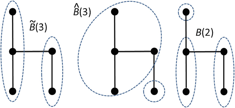
Two minimal 3-coverings and a minimal 2-covering for the chair network
which shows two minimal 3-coverings and a minimal 2-covering. Choosing q = 2, for the covering  from (17.1) we have
  , while for
  we have
  . For
. For  we have
  . If we use
  , then from (17.3) and the range s ∈ [2, 3] we obtain
  . If instead we use
  and the same range of s we obtain
  . Thus the method of [Wang 11] can yield different values of D
2 depending on the minimal covering selected. □
. Thus the method of [Wang 11] can yield different values of D
2 depending on the minimal covering selected. □
 is largest. It is well-known that entropy is maximized when all the probabilities are equal. Theorem 17.1 below, concerning a continuous optimization problem, proves that the partition function is minimized when the probabilities are equal.
For integer J ≥ 2, let
is largest. It is well-known that entropy is maximized when all the probabilities are equal. Theorem 17.1 below, concerning a continuous optimization problem, proves that the partition function is minimized when the probabilities are equal.
For integer J ≥ 2, let  denote the continuous optimization problem
 is p
j = 1∕J for each j, and the optimal objective function value is J
1−q.
is p
j = 1∕J for each j, and the optimal objective function value is J
1−q.Proof [
Rosenberg 17b] If p
j = 1 for some j, then for each other j we have p
j = 0 and the objective function value is 1. Next, suppose each p
j > 0 in the solution of  . Let λ be the Lagrange multiplier associated with the constraint
  . The first order optimality condition for p
j is
. The first order optimality condition for p
j is  . Thus each p
j has the same value, which is 1∕J. The corresponding objective function value is
. Thus each p
j has the same value, which is 1∕J. The corresponding objective function value is  . This value is less than the value 1 (obtained when exactly one p
j = 1) when J
1−q < 1, which holds for q > 1. For q > 1 and p > 0, the function p
q is a strictly convex function of p, so p
j = 1∕J is the unique global (as opposed to only a local) solution of
. This value is less than the value 1 (obtained when exactly one p
j = 1) when J
1−q < 1, which holds for q > 1. For q > 1 and p > 0, the function p
q is a strictly convex function of p, so p
j = 1∕J is the unique global (as opposed to only a local) solution of  . Finally, suppose that for some solution of
  we have p
j ∈ [0, 1) for each j, but the number of positive p
j is J
0, where J
0 < J. The above arguments show that the optimal objective function value is
we have p
j ∈ [0, 1) for each j, but the number of positive p
j is J
0, where J
0 < J. The above arguments show that the optimal objective function value is  . Since for q > 1 we have
  , any solution of
  must have p
j > 0 for each j. □
must have p
j > 0 for each j. □
Applying Theorem 17.1 to  , minimizing the partition function
  over all minimal s-coverings of
  yields a minimal s-covering for which all the probabilities p
j(s) are approximately equal. Since p
j(s) = N
j(s)∕N, having the box probabilities almost equal means that all boxes in the minimal s-covering have approximately the same number of nodes. The following definition of an (s, q) minimal covering, for use in computing D
q, is analogous to the definition in [Rosenberg 17a] of a maximal entropy minimal covering, for use in computing d
I.
yields a minimal s-covering for which all the probabilities p
j(s) are approximately equal. Since p
j(s) = N
j(s)∕N, having the box probabilities almost equal means that all boxes in the minimal s-covering have approximately the same number of nodes. The following definition of an (s, q) minimal covering, for use in computing D
q, is analogous to the definition in [Rosenberg 17a] of a maximal entropy minimal covering, for use in computing d
I.
Definition 17.1 [
Rosenberg 17b] For  , the covering
  of
of  is an (s, q) minimal covering if (i)
  is a minimal s-covering and (ii) for any other minimal s-covering
  we have
  . □
. □
Procedure 17.1 below shows how an (s, q) minimal covering can be computed, for a given s and q, by a simple modification of whatever box-counting method is used to compute a minimal s-covering.
Procedure 17.1 Let  be the best s-covering obtained over all executions of whatever box-counting method is utilized. Suppose we have executed box counting some number of times, and stored
  and
and  , so
, so  is the current best estimate of the minimal value of the partition function. Now suppose we execute box counting again, and generate a new s-covering
  using B(s) boxes. Let
  be the partition function value associated with
  . If
. If  holds, or if
  and
and  hold, set
  and
and  . □
. □
Let s be fixed. Procedure 17.1 shows that we can easily modify any box-counting method to compute the (s, q) minimal covering for a given q. However, this approach to eliminating ambiguity in the computation of D q is not attractive, since it requires computing an (s, q) minimal covering for each value of q for which we wish to compute D q. Moreover, since there are only a finite number of minimal s-coverings, as q varies we will eventually rediscover some (s, q) minimal coverings, that is, for some q 1 and q 2 we will find that the (s, q 1) minimal covering is identical to the (s, q 2) minimal covering. An elegant alternative to computing an (s, q) minimal covering for each s and q, while still achieving our goal of unambiguously computing D q, is to use lexico minimal summary vectors.
For a given box size s, we summarize an s-covering  by the point
  , where J ≡ B(s), where x
j(s) = N
j(s) for 1 ≤ j ≤ J, and where x
1(s) ≥ x
2(s) ≥⋯ ≥ x
J(s). We say “summarize” since x(s) does not specify all the information in
, where J ≡ B(s), where x
j(s) = N
j(s) for 1 ≤ j ≤ J, and where x
1(s) ≥ x
2(s) ≥⋯ ≥ x
J(s). We say “summarize” since x(s) does not specify all the information in  ; in particular,
  specifies exactly which nodes belong to each box, while x(s) specifies only the number of nodes in each box. We use the notation
  to mean that x(s) summarizes the s-covering
  and that x
1(s) ≥ x
2(s) ≥⋯ ≥ x
J(s). For example, if N = 37, s = 3, and B(3) = 5, then we might have
and that x
1(s) ≥ x
2(s) ≥⋯ ≥ x
J(s). For example, if N = 37, s = 3, and B(3) = 5, then we might have  for x(s) = (18, 7, 5, 5, 2). However, we cannot have
  for x(s) = (7, 18, 5, 5, 2) since the components of x(s) are not ordered correctly. If
  , then each x
j(s) is positive, since x
j(s) is the number of nodes in box B
j. We call
, then each x
j(s) is positive, since x
j(s) is the number of nodes in box B
j. We call  a summary vector of
  . By “x(s) is a summary vector” we mean x(s) summarizes some
  .
.
Let  for some positive integer K. Let
  be the point obtained by deleting the first component of x. For example, if x = (18, 7, 5, 5, 2), then right(x) = (7, 5, 5, 2). Similarly, we define right
2(x) ≡ right(right(x)), so right
2(7, 7, 5, 2) = (5, 2). Let
be the point obtained by deleting the first component of x. For example, if x = (18, 7, 5, 5, 2), then right(x) = (7, 5, 5, 2). Similarly, we define right
2(x) ≡ right(right(x)), so right
2(7, 7, 5, 2) = (5, 2). Let  and
and  be numbers. We say that u ≽ v (in words, u is lexico greater than or equal to v) if ordinary inequality holds, that is, u ≽ v if u ≥ v. (We use lexico instead of the longer lexicographically.) Thus 6 ≽ 3 and 3 ≽ 3. Now let
  and
and  . We define lexico inequality recursively. We say that y ≽ x if either (i) y
1 > x
1 or (ii) y
1 = x
1 and right(y) ≽ right(x). For example, for x = (9, 6, 5, 5, 2), y = (9, 6, 4, 6, 2), and z = (8, 7, 5, 5, 2), we have x ≽ y and x ≽ z and y ≽ z.
. We define lexico inequality recursively. We say that y ≽ x if either (i) y
1 > x
1 or (ii) y
1 = x
1 and right(y) ≽ right(x). For example, for x = (9, 6, 5, 5, 2), y = (9, 6, 4, 6, 2), and z = (8, 7, 5, 5, 2), we have x ≽ y and x ≽ z and y ≽ z.
Definition 17.2 Let  . Then x(s) is lexico minimal if (i)
  is a minimal s-covering and (ii) if
  is a minimal s-covering distinct from
  and
and  , then y(s) ≽ x(s). □
Theorem 17.2 For each s there is a unique lexico minimal summary vector.
Proof [
Rosenberg 17b] Pick s. Since there are only a finite number of minimal s-coverings of  , and the corresponding summary vectors can be ordered using lexicographic ordering, then a lexico minimal summary vector exists. To show that there is unique lexico minimal summary vector, suppose that
  and
and  are both lexico minimal. Define J ≡ B(s), so J is the number of boxes in both
  and in
  . If J = 1, then a single box covers
  , and that box must be
  itself, so the theorem holds. So assume J > 1. If x
1(s) > y
1(s) or x
1(s) < y
1(s), then x(s) and y(s) cannot both be lexico minimal, so we must have x
1(s) = y
1(s). We apply the same reasoning to right(x(s)) and right(y(s)) to conclude that x
2(s) = y
2(s). If J = 2 we are done; the theorem is proved. If J > 2, we apply the same reasoning to right
2(x(s)) and right
2(y(s)) to conclude that x
3(s) = y
3(s). Continuing in this manner, we finally obtain x
J(s) = y
J(s), so x(s) = y(s). □
itself, so the theorem holds. So assume J > 1. If x
1(s) > y
1(s) or x
1(s) < y
1(s), then x(s) and y(s) cannot both be lexico minimal, so we must have x
1(s) = y
1(s). We apply the same reasoning to right(x(s)) and right(y(s)) to conclude that x
2(s) = y
2(s). If J = 2 we are done; the theorem is proved. If J > 2, we apply the same reasoning to right
2(x(s)) and right
2(y(s)) to conclude that x
3(s) = y
3(s). Continuing in this manner, we finally obtain x
J(s) = y
J(s), so x(s) = y(s). □
 and
and  , define
Lemma 17.1 Let α, β, and γ be positive numbers. Then (α + β)∕(α + γ) > 1 if and only if β > γ.
Theorem 17.3 Let  . If x(s) is lexico minimal, then
  is (s, q) minimal for all sufficiently large q.
 be lexico minimal. Let
  be a minimal s-covering distinct from
  , and let
  . By Theorem 17.2, y(s) ≠ x(s). Define J ≡ B(s). Consider the ratio

 . Since
  and
and  are minimal s-coverings, and since x(s) is lexico minimal, then y
k(s) > x
k(s). We have
are minimal s-coverings, and since x(s) is lexico minimal, then y
k(s) > x
k(s). We have 
Analogous to Procedure 17.1, Procedure 17.2 below shows how, for a given s, the lexico minimal x(s) can be computed by a simple modification of whatever box-counting method is used to compute a minimal s-covering.
Procedure 17.2 Let  be the best s-covering obtained over all executions of whatever box-counting method is utilized. Suppose we have executed box counting some number of times, and stored
  and
and  , so
, so  is the current best estimate of a lexico minimal summary vector. Now suppose we execute box counting again, and generate a new s-covering
  using B(s) boxes. Let
  . If
. If  holds, or if
  and
and  hold, set
  and
and  . □
. □
Procedure 17.2 shows that the only additional steps, beyond the box- counting method itself, needed to compute x(s) are lexicographic comparisons, and no evaluations of the partition function  are required. Theorem 17.2 proved that x(s) is unique. Theorem 17.3 proved that x(s) is “optimal” (i.e., (s, q) minimal) for all sufficiently large q. Thus an attractive way to unambiguously compute D
q is to compute x(s) for a range of s and use the x(s) summary vectors to compute D
q, using Definition 17.3 below.
are required. Theorem 17.2 proved that x(s) is unique. Theorem 17.3 proved that x(s) is “optimal” (i.e., (s, q) minimal) for all sufficiently large q. Thus an attractive way to unambiguously compute D
q is to compute x(s) for a range of s and use the x(s) summary vectors to compute D
q, using Definition 17.3 below.
 has the generalized dimension D
q if for some constant c, for some positive integers L and U satisfying 2 ≤ L < U ≤ Δ, and for each integer s ∈ [L, U],
has the generalized dimension D
q if for some constant c, for some positive integers L and U satisfying 2 ≤ L < U ≤ Δ, and for each integer s ∈ [L, U], 
 is lexico minimal. □
Other than the minor detail that (17.3) is formulated using radius-based boxes rather than diameter-based boxes, (17.6) is identical to (17.3). Definition 17.3 modifies the definition of D q in [Wang 11] to ensure uniqueness of D q. Since x(s) summarizes a minimal s-covering, using x(s) to compute D q, even when q is not sufficiently large as required by Theorem 17.3, introduces no error in the computation of D q. By using the summary vectors x(s) we can unambiguously compute D q, with negligible extra computational burden.
Example 17.
1
(Continued) Consider again the chair network of Fig. 17.1. Choose q = 2. For s = 2 we have  and
and  . For s = 3 we have
  and
and  . Choose L = 2 and U = 3. From Definition 17.3 we have
  . □
. □
Definition 17.4 If for some constant d we have D
q = d for  , then
  is monofractal; if
  is not monofractal, then
  is multifractal. □
 be lexico minimal and let x
1(s) be the first element of x(s). Let m(s) be the multiplicity of x
1(s), defined to be the number of occurrences of x
1(s) in x(s). (For example, if x(s) = (7, 7, 6, 5, 4), then x
1(s) = 7 and m(s) = 2 since there are two occurrences of 7.) Then x
1(s) > x
j(s) for j > m(s). Using (17.4), we have
be lexico minimal and let x
1(s) be the first element of x(s). Let m(s) be the multiplicity of x
1(s), defined to be the number of occurrences of x
1(s) in x(s). (For example, if x(s) = (7, 7, 6, 5, 4), then x
1(s) = 7 and m(s) = 2 since there are two occurrences of 7.) Then x
1(s) > x
j(s) for j > m(s). Using (17.4), we have 


 .
Having constructed
.
Having constructed  , the task is to color the nodes of
  , using the minimal number of colors, such that no arc in
  connects nodes assigned the same color. The heuristic used to color
  is the following. Suppose we have ordered the
  nodes in some order n
1, n
2, …, n
N. Define
nodes in some order n
1, n
2, …, n
N. Define  . For
. For  , let
, let  be the set of nodes in
  that are adjacent to node n
i. (This set is empty if n
i is an isolated node.) Let c(n) be the color assigned to node n. Initialize c(n
1) = 1 and c(n) = 0 for all other nodes. For i = 2, 3, …, N, the color c(n
i) assigned to n
i is the smallest color not assigned to any neighbor of n
i:
that are adjacent to node n
i. (This set is empty if n
i is an isolated node.) Let c(n) be the color assigned to node n. Initialize c(n
1) = 1 and c(n) = 0 for all other nodes. For i = 2, 3, …, N, the color c(n
i) assigned to n
i is the smallest color not assigned to any neighbor of n
i: 
 , which is also the estimate of B(s), is
  , the number of colors used to color the auxiliary graph. All nodes with the same color belong to the same box.
This node coloring heuristic assumes some given ordering of the nodes. Many random orderings of the nodes were generated: for the dolphins
and jazz networks 10N
random orderings of the nodes were generated, and for the C. elegans network N random orderings were generated. The node coloring heuristic was executed for each random ordering. Random orderings were obtained by starting with the permutation array π(n) = n, picking two random integers  , and swapping the contents of π in positions i and j. For the dolphins and jazz networks 10N swaps were executed to generate each random ordering, and for the C. elegans network N swaps were executed. In the plots for these three networks, the horizontal axis is
  , the red line plots
  versus
  , and the blue line plots
  versus
  .
.
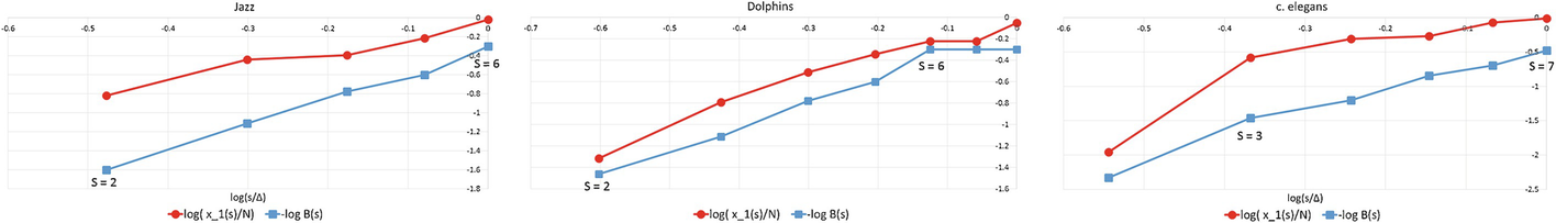
D ∞ for three networks
The red and blue plots are over the range 2 ≤ s ≤ 6. Over this range, a linear fit to the red plot yields, from (17.9), D ∞ = 1.55, and a linear fit to the blue plot yields d B = 1.87. Since d B = D 0, we have D 0 > D ∞.
Example 17.3 Figure 17.2 (middle) provides results for the dolphins network (introduced in Example 7.2), with 62 nodes, 159 arcs, and Δ = 8. The red and blue plots are over the range 2 ≤ s ≤ 8. Using (17.9), a linear fit to the red plot over 2 ≤ s ≤ 6 (the portion of the plots that appears roughly linear) yields D ∞ = 2.29, and a linear fit to the blue plot over 2 ≤ s ≤ 6 yields d B = 2.27, so D ∞ very slightly exceeds d B.
Example 17.4 Figure 17.2 (right) provides results for the C. elegans network, with 453 nodes, 2040 arcs, and Δ = 7. This is the unweighted, undirected version of the neural network of C. elegans [Newman]. The red and blue plots are over the range 2 ≤ s ≤ 7. Using (17.9), a linear fit to the red plot over 3 ≤ s ≤ 7 (the portion of the plots that appears roughly linear) yields D ∞ = 1.52, and a linear fit to the blue plot over 3 ≤ s ≤ 7 yields d B = 1.73, so D 0 > D ∞.
In each of the three figures, the two lines roughly begin to intersect as s∕Δ increases. This occurs since x 1(s) is non-decreasing in s and x 1(s)∕N = 1 for s > Δ; similarly B(s) is non-increasing in s and B(s) = 1 for s > Δ.
Exercise 17.1 An arc-covering based approach, e.g., [Jalan 17, Zhou 07], can be used to define D
q, where p
j(s) is the fraction of all arcs contained in box  . Compare the D
q values obtained using arc-coverings with the D
q values obtained using node-coverings. □
. Compare the D
q values obtained using arc-coverings with the D
q values obtained using node-coverings. □
Exercise 17.2 Compute D q for integer q in [−10, 10] for the hub and spoke with a tail network of Example 15.2. □
17.2 Non-monotonicity of the Generalized Dimensions
For a geometric object, we showed (Theorem 16.1) that the generalized dimensions D q are monotone non-increasing in q. In this section we show that, for a network, the generalized dimensions can fail to be monotone non-increasing in q, even when D q is computed using the lexico minimal summary vectors x(s). (The fact that D q can be increasing in q for q < 0, or for small positive values of q, was observed in [Wang 11]. For example, for the protein-protein interaction networks studied in [Wang 11], D q is increasing in q for q ∈ [0, 1], and D q peaks at q ≈ 2.) Moreover, in this section we show that D q versus q curve can assume different shapes, depending on the range of box sizes used to compute D q.
 is a lexico minimal summary vector for box size s. In Sect. 17.1, we showed that to compute D
q for a given q, we identify a range [L, U] of box sizes, where L < U, such that
is a lexico minimal summary vector for box size s. In Sect. 17.1, we showed that to compute D
q for a given q, we identify a range [L, U] of box sizes, where L < U, such that  is approximately linear in
  for s ∈ [L, U]. The estimate of D
q is 1∕(q − 1) times the slope of the linear approximation. More formally, Definition 17.3 required D
q to satisfy
for s ∈ [L, U]. The estimate of D
q is 1∕(q − 1) times the slope of the linear approximation. More formally, Definition 17.3 required D
q to satisfy 
 and
and  . For the 3-covering
  we have
  and
and  . With L = 2 and U = 3, from (17.6) we have
 then
then  and
and  . With L = 2 and U = 3, but now using
  instead of
  , we obtain
 versus q, and
  versus q over the range 0 ≤ q ≤ 15.
Two plots of the generalized dimensions of the chair network
Neither curve is monotone non-increasing: the  curve is unimodal, with a local minimum at q ≈ 4.1, and the
  curve is monotone increasing. □
In Example 17.5, since (4, 1) ≽ (3, 2) then x(3) = (3, 2) is the lexico minimal summary vector for s = 3. Using the x(s) vectors eliminates one source of ambiguity in computing D q. However, there is yet another source of ambiguity: the selection of the range of box sizes used to compute D q. What has not been previously recognized is that for a network the choice of L and U can dramatically change the shape of the D q versus q curve [Rosenberg 17c]; this is the subject of the remainder of this section.
 is approximately linear in
  , and then use (17.10) to estimate D
q, e.g., using linear regression. With this approach, to report computational results to other researchers it would be necessary to specify, for each q, the range of box sizes used to estimate D
q. This is certainly not the protocol currently followed in research on generalized dimensions. Instead, the approach taken in [Wang 11] and [Rosenberg 17c] was to pick a single L and U and estimate D
q for all q with this L and U. Moreover, rather than using a technique such as linear regression to estimate D
q over the range [L, U] of box sizes, in [Rosenberg 17c] D
q was estimated using only the two box sizes L and U.1 With this two-point approach, the estimate of D
q is the slope of the secant line connecting the point
, and then use (17.10) to estimate D
q, e.g., using linear regression. With this approach, to report computational results to other researchers it would be necessary to specify, for each q, the range of box sizes used to estimate D
q. This is certainly not the protocol currently followed in research on generalized dimensions. Instead, the approach taken in [Wang 11] and [Rosenberg 17c] was to pick a single L and U and estimate D
q for all q with this L and U. Moreover, rather than using a technique such as linear regression to estimate D
q over the range [L, U] of box sizes, in [Rosenberg 17c] D
q was estimated using only the two box sizes L and U.1 With this two-point approach, the estimate of D
q is the slope of the secant line connecting the point  to the point
  , where x(L) and x(U) are the lexico minimal summary vectors for box sizes L and U, respectively. Using (17.4) and (17.10), the estimate of D
q is D
q(L, U), defined by
, where x(L) and x(U) are the lexico minimal summary vectors for box sizes L and U, respectively. Using (17.4) and (17.10), the estimate of D
q is D
q(L, U), defined by ![$$\displaystyle \begin{aligned} D_q(L, U) &\equiv \frac { \log Z\big(x(U), q\big) - \log Z\big(x(L), q\big) } { (q-1)\big( \log(U/\varDelta) - \log(L/\varDelta) \big) }\\ &= \frac{1} {\log(U/L) (q-1) } \log \left( \frac{\sum_{B_{{j}} \in {\mathcal{B}}(U)} [x_{{j}}(U)]^q } {\sum_{B_{{j}} \in {\mathcal{B}}(L)} [x_{{j}}(L)]^q } \right) \, . {} \end{aligned} $$](../images/487758_1_En_17_Chapter/487758_1_En_17_Chapter_TeX_Equ15.png)
 curve is approximately linear for 2 ≤ s ≤ 6.
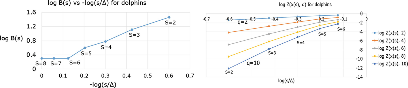
Box counting and  versus
  for the dolphins network
 versus
  for 2 ≤ s ≤ 6 and for q = 2, 4, 6, 8, 10 (q = 2 is the top curve, and q = 10 is the bottom curve). This figure shows that, although the
  versus
  curves are less linear as q increases, a linear approximation is quite reasonable. Moreover, we are particularly interested, in the next section, in the behavior of the
  versus
  curve for small positive q, the region where the linear approximation is best. Using (17.13), Fig. 17.5 plots the secant estimate D
q(L, U) versus q for various choices of L and U.
curve for small positive q, the region where the linear approximation is best. Using (17.13), Fig. 17.5 plots the secant estimate D
q(L, U) versus q for various choices of L and U.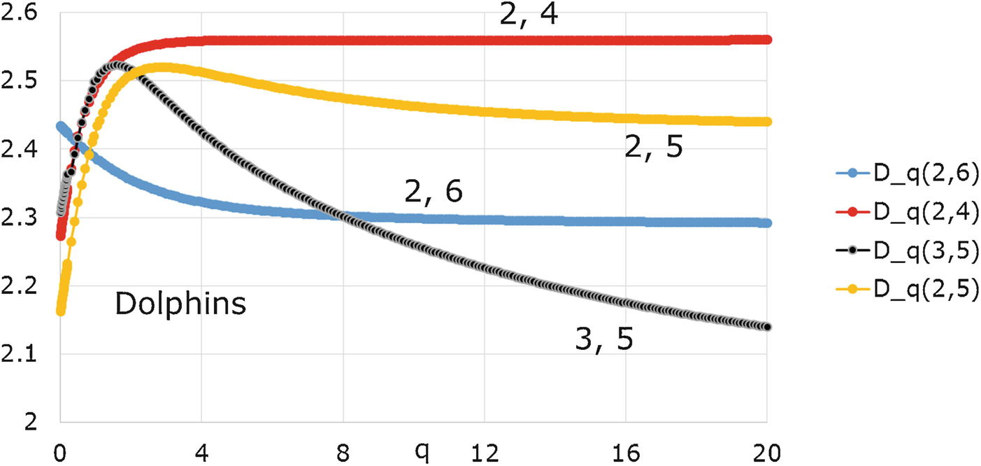
Secant estimate of D q for the dolphins network for different L and U
Since the D q versus q curve for a geometric multifractal is monotone non-increasing, it is remarkable that different choices of L and U lead to such different shapes for the D q(L, U) versus q curve.
 denote the first derivative with respect to q of D
q(L, U), evaluated at q = 0. A simple closed-form expression for
denote the first derivative with respect to q of D
q(L, U), evaluated at q = 0. A simple closed-form expression for  was derived in [Rosenberg 17c]. For box size s, let
  summarize the minimal s-covering
  . Define
 , then

 ) and define K ≡ B(U). For simplicity of notation, by ∑j we mean
  and by ∑k we mean
  . Similarly, by ∏j we mean
  and by ∏k we mean
  . Assume that
  means the natural log. For 1 ≤ j ≤ J, define a
j ≡ x
j(L) and
means the natural log. For 1 ≤ j ≤ J, define a
j ≡ x
j(L) and  . For 1 ≤ k ≤ K, define b
k ≡ x
k(U) and
. For 1 ≤ k ≤ K, define b
k ≡ x
k(U) and  . Define
  . For simplicity of notation, define F(q) ≡ D
q(L, U). By F
′(0) we mean the first derivative of F(q) evaluated at q = 0, so
. For simplicity of notation, define F(q) ≡ D
q(L, U). By F
′(0) we mean the first derivative of F(q) evaluated at q = 0, so  . Using the above notation and definitions, from (17.13) we have
 . We have f
1(0) = f
2(0) = J. Evaluating the first derivatives at q = 0, we have
. We have f
1(0) = f
2(0) = J. Evaluating the first derivatives at q = 0, we have  and
and  . Since f
1(q) and f
2(q) have the same function values and first derivatives at q = 0, then F(0) = M(0) and F
′(0) = M
′(0), where M(q) is defined by
. Since f
1(q) and f
2(q) have the same function values and first derivatives at q = 0, then F(0) = M(0) and F
′(0) = M
′(0), where M(q) is defined by 

![$$\displaystyle \begin{aligned} \begin{array}{rcl} M^{\prime}(q) {=} \frac{\omega} {(q-1)^2 } \left[ \frac {(q-1) (1/J) \sum_k [ e^{({\beta}_{{k}}-\alpha) q}({\beta}_{{k}} - \alpha)]} { (1/J) \sum_k e^{({\beta}_{{k}}-\alpha) q} } {-}\log \left( \frac{1}{J} \sum_k e^{({\beta}_{{k}}-\alpha) q} \right) \right] \, . \end{array} \end{aligned} $$](../images/487758_1_En_17_Chapter/487758_1_En_17_Chapter_TeX_Equ21.png)

□
Theorem 17.4 says that the slope of the secant estimate of D q at q = 0 depends on x(L) and x(U) only through the ratio of the geometric mean to the arithmetic mean of the components of x(L), and similarly for x(U). Note that the proof of Theorem 17.4 does not require x(s) to be lexico minimal. Since U > L, Theorem 17.4 immediately implies the following corollary.
Corollary 17.1  if and only if R(L) > R(U), and
  if and only if R(L) < R(U). □
For a given L and U, Theorem 17.5 below provides a sufficient condition for D q(L, U) to have a local maximum or minimum.
Theorem 17.5 [
Rosenberg 17c] Assume (17.10) holds as an equality. If x(s) is a lexico minimal summary vector summarizing the minimal s-covering  , then (i) if R(L) > R(U) and B(L)∕B(U) > x
1(U)∕x
1(L), then D
q(L, U) has a local maximum at some q > 0. (ii) If R(L) < R(U) and B(L)∕B(U) < x
1(U)∕x
1(L), then D
q(L, U) has a local minimum at some q > 0.
, then (i) if R(L) > R(U) and B(L)∕B(U) > x
1(U)∕x
1(L), then D
q(L, U) has a local maximum at some q > 0. (ii) If R(L) < R(U) and B(L)∕B(U) < x
1(U)∕x
1(L), then D
q(L, U) has a local minimum at some q > 0.
 , where x
1(s) is the first coordinate of the lexico minimal summary vector x(s). Defining
, where x
1(s) is the first coordinate of the lexico minimal summary vector x(s). Defining  , we have

 and D
0 > D
∞, then D
q(L, U) must have a local maximum at some positive q. By Corollary 17.1, if R(L) > R(U) then
and D
0 > D
∞, then D
q(L, U) must have a local maximum at some positive q. By Corollary 17.1, if R(L) > R(U) then  . By (17.18) and (17.19), if B(L)∕B(U) > x
1(U)∕x
1(L), then D
0 > D
∞. □
. By (17.18) and (17.19), if B(L)∕B(U) > x
1(U)∕x
1(L), then D
0 > D
∞. □Example 17.7 To illustrate Theorem 17.5, consider again the dolphins network
of Example 17.2 with L = 3 and U = 5. We have B(3) = 13, B(5) = 4, x
1(3) = 10, and x
1(5) = 28, so  and
and  . We have R(3) = 0.773, R(5) = 0.660, and
  , so D
q(3, 5) has a local maximum, as seen in Fig. 17.5. Moreover, for the dolphins network, choosing L = 2 and U = 5 we have
, so D
q(3, 5) has a local maximum, as seen in Fig. 17.5. Moreover, for the dolphins network, choosing L = 2 and U = 5 we have  , and
, and  , so D
0 < D
∞, as is evident from Fig. 17.5. Thus the inequality D
0 ≥ D
∞, which is valid for geometric multifractals, does not hold for the dolphins network
with L = 2 and U = 5. □
, so D
0 < D
∞, as is evident from Fig. 17.5. Thus the inequality D
0 ≥ D
∞, which is valid for geometric multifractals, does not hold for the dolphins network
with L = 2 and U = 5. □
 is a monofractal but not a multifractal. To see this, suppose all boxes in
  have the same mass, and that all boxes in
  have the same mass. Then for s ∈{L, U} we have x
j(s) = N∕B(s) for 1 ≤ j ≤ B(s), and (17.4) yields
have the same mass. Then for s ∈{L, U} we have x
j(s) = N∕B(s) for 1 ≤ j ≤ B(s), and (17.4) yields ![$$\displaystyle \begin{aligned} Z\big(x(s), q \big) = \sum_{B_{{j}} \in {\mathcal{B}}(s)} \left(\frac{x_{{j}}(s)}{N} \right)^q = \sum_{B_{{j}} \in {\mathcal{B}}(s)} \left( \frac{1}{B(s)} \right) ^{q} = [B(s)]^{1-q} \, . \end{aligned}$$](../images/487758_1_En_17_Chapter/487758_1_En_17_Chapter_TeX_Equg.png)
![$$\displaystyle \begin{aligned} D_q &= \frac{\log Z\big( (x(U), q \big)- \log Z\big(x(L), q \big)} {(q-1)\big( \log U - \log L \big)} \; = \; \frac{ \log \big( [B(U)]^{1-q} \big) {-} \log \big( [B(L)]^{1-q} \big)} {(q-1) \big( \log U - \log L \big)} \\ &{=} \frac{ \log B(L) {-} \log B(U)} {\log U - \log L} \; = \; D_0 \; = \; d_{{B}} \, , {} \end{aligned} $$](../images/487758_1_En_17_Chapter/487758_1_En_17_Chapter_TeX_Equ24.png)
 is a monofractal. Thus equal box masses imply
  is a monofractal, the simplest of all fractal structures.
There are several ways to try to obtain equal box masses in a minimal s-covering of  . As discussed in Chap. 15, ambiguity in the choice of minimal coverings used to compute d
I is eliminated by maximizing entropy. Since the entropy of a probability distribution is maximized when all the probabilities are equal, a maximal entropy minimal covering equalizes (to the extent possible) the box masses. Similarly, ambiguity in the choice of minimal s-coverings used to compute D
q is eliminated by minimizing the partition function
. As discussed in Chap. 15, ambiguity in the choice of minimal coverings used to compute d
I is eliminated by maximizing entropy. Since the entropy of a probability distribution is maximized when all the probabilities are equal, a maximal entropy minimal covering equalizes (to the extent possible) the box masses. Similarly, ambiguity in the choice of minimal s-coverings used to compute D
q is eliminated by minimizing the partition function  . Since, by Theorem 17.3, for all sufficiently large q the unique lexico minimal vector x(s) summarizes the s-covering that minimizes
  , and since, by Theorem 17.1, for q > 1 a partition function is minimized when all the probabilities are equal, then x(s) also equalizes (to the extent possible) the box masses. Theorem 17.4 suggests a third way to try to equalize the masses of all boxes in a minimal s-covering: since G(s) ≤ A(s) and G(s) = A(s) when all boxes have the same mass, a minimal s-covering that maximizes G(s) will also equalize (to the extent possible) the box masses. The advantage of computing the lexico minimal summary vectors x(s), rather than maximizing the entropy or maximizing G(s), is that x(s) is provably unique. We now apply Theorem 17.4 to the chair network of Example 17.1, to the dolphins network of Example 17.3, and to two other networks.
Example 17.8 For the chair network
we have L = 2, x(L) = (2, 2, 1), U = 3, and x(U) = (3, 2). We have  , as shown in Fig. 17.3 by the slightly negative slope of the lower curve at q = 0. As illustrated in Fig. 17.3, this curve is not monotone non-increasing; it has a local minimum. □
 for various choices of L and U.
 for the dolphins network
L, U |
|
2, 6 | − 0.056 |
3, 5 | 0.311 |
2, 4 | 0.393 |
2, 5 | 0.367 |

 versus
  . For example, for (L, U) = (2, 6) we have
  , as illustrated by the slightly positive slope of the dashed red line in Fig. 17.6, since the slope of the dashed red line is
  . For the other choices of (L, U) in Table 17.1, the values of
  are positive and roughly equal.
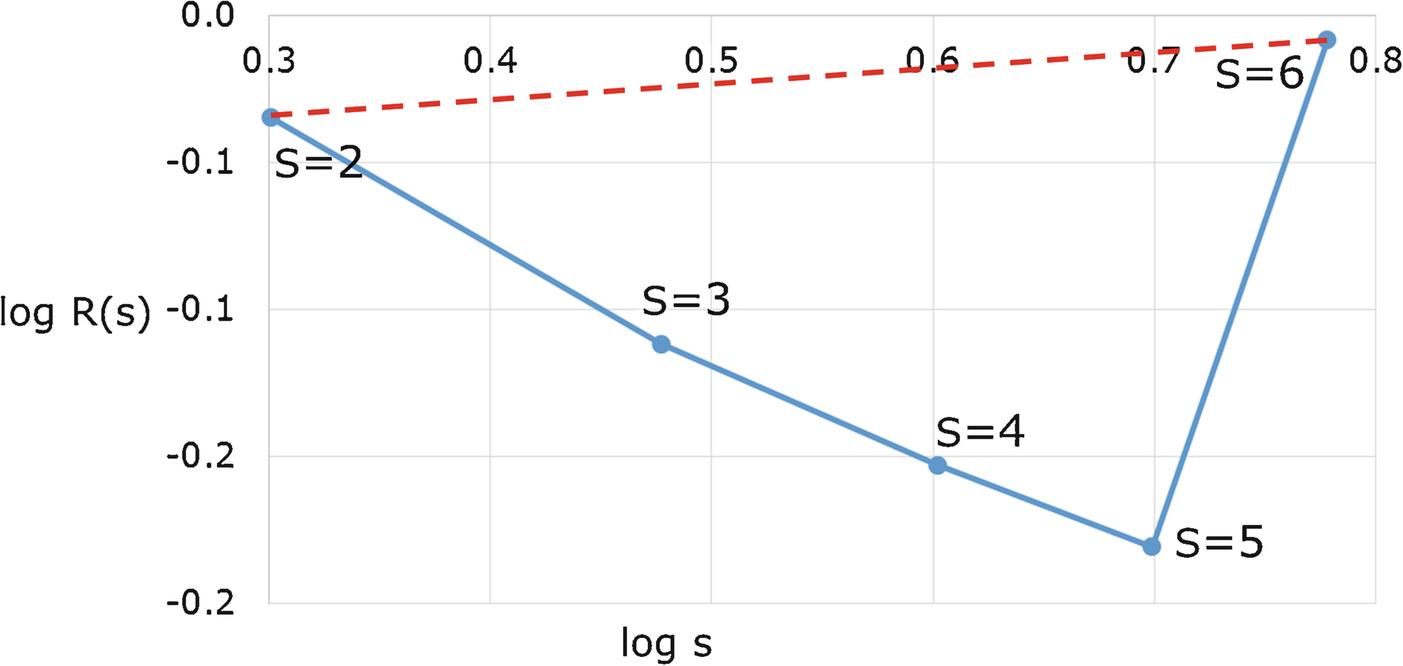
 versus
  for the dolphins network
Figure 17.4 (right) visually suggests that  is better approximated by a linear fit over s ∈ [2, 5] than over s ∈ [2, 6], and Fig. 17.6 clearly shows that s = 6 is an outlier in that using U = 6 dramatically changes
  . □
. □
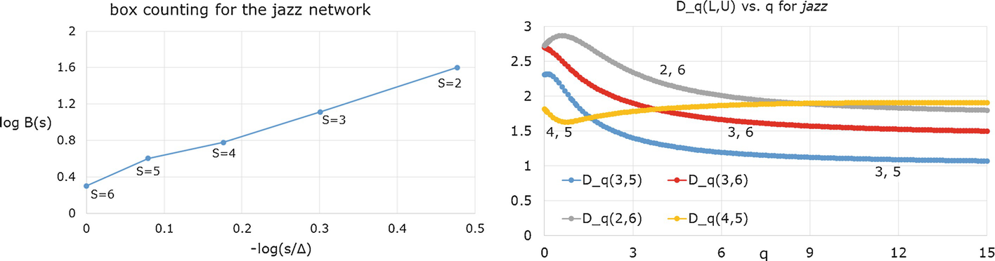
jazz box counting (left) and D q versus q for various L, U (right)
 , D
0, and D
∞ for nine choices of L and U; the rows are sorted by decreasing
, D
0, and D
∞ for nine choices of L and U; the rows are sorted by decreasing  .
. Results for the jazz network for various L and U
L, U |
| D 0 | D ∞ |
2, 3 | 1.576 | 2.77 | 2.16 |
2, 4 | 1.224 | 2.74 | 1.42 |
2, 5 | 0.826 | 2.51 | 1.51 |
3, 4 | 0.728 | 2.69 | 0.37 |
2, 6 | 0.485 | 2.73 | 1.68 |
3, 5 | 0.231 | 2.31 | 1.00 |
3, 6 | − 0.154 | 2.70 | 1.40 |
4, 5 | − 0.411 | 1.82 | 1.82 |
5, 6 | − 1.232 | 3.80 | 2.52 |

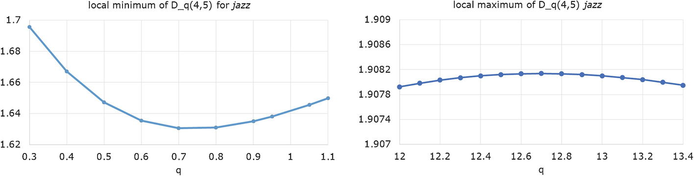
Local minimum and maximum of D q for the jazz network and L = 4, U = 5


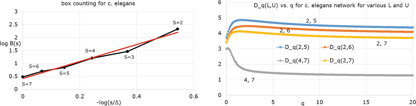
C. elegans box counting (left) and D q(L, U) versus q for various L, U (right)
The results of this section, and of Sect. 17.1 above, show that two requirements should be met when reporting fractal dimensions of a network. First, since there are in general multiple minimal s-coverings, and these different coverings can yield different values of D
q, computational results should specify the rule (e.g., a maximal entropy covering, or a covering yielding a lexico minimal summary vector) used to unambiguously select a minimal s-covering. Second, the lower bound L and upper bound U on the box sizes used to compute D
q should also be reported. Published values of D
q not meeting these two requirements cannot in general be considered benchmarks. As to the values of L and U yielding the most meaningful results, it is desirable to identify the largest range [L, U] over which  is approximately linear in
  ; this is a well-known principle in the estimation of fractal dimensions. Future research may uncover other criteria for selecting the “best” L and U.
The numerical results from [Rosenberg 17c] presented in this section suggest several additional avenues for investigation. (1) We conjecture that D q(L, U) can have at most one local maximum and one local minimum. (2) Under what conditions does D q(L, U) have two critical points? (3) Derive closed-form bounds q 1 and q 2, easily obtainable from x(L) and x(U), such that if q ⋆ is a critical point of D q(L, U) then q 1 ≤ q ⋆ ≤ q 2.
17.3 Multifractal Network Generator
A method for generating a network from a multifractal measure was proposed in [Palla 10], and the implementation of this method was considered in more detail in [Horváth 13]. The method has two parts: generating the multifractal measure, and generating the network from the measure.
To generate the measure, start with the unit square [0, 1] × [0, 1], which for brevity we denote by [0, 1]2. Pick an integer m ≥ 2 and divide [0, 1]2 into m pieces, using m − 1 vertical slices. For example, with m = 3 we might slice [0, 1]2 at the x values  and
and  . Call this set of m − 1 numbers, e.g.,
  , the “V-slicing ratios”. Now slice [0, 1]2 using m − 1 horizontal slices, where the spacing of the horizontal slices can differ from that of the vertical slices. For example, we might slice [0, 1]2 horizontally at the y values
  and
and  . Call this set of m − 1 numbers, e.g.,
  , the “H-slicing ratios”. The net effect of these 2(m − 1) slices is to partition [0, 1]2 into m
2 “generation 1” rectangles.
, the “H-slicing ratios”. The net effect of these 2(m − 1) slices is to partition [0, 1]2 into m
2 “generation 1” rectangles.
 . The probabilities need not have any relation to the values of the slicing ratios. This concludes the first iteration of the construction of the multifractal measure. Figure 17.11 (left) illustrates the generation-1 construction for m = 3 and for the case where the H-slicing ratios and V-slicing ratios are both
  .
.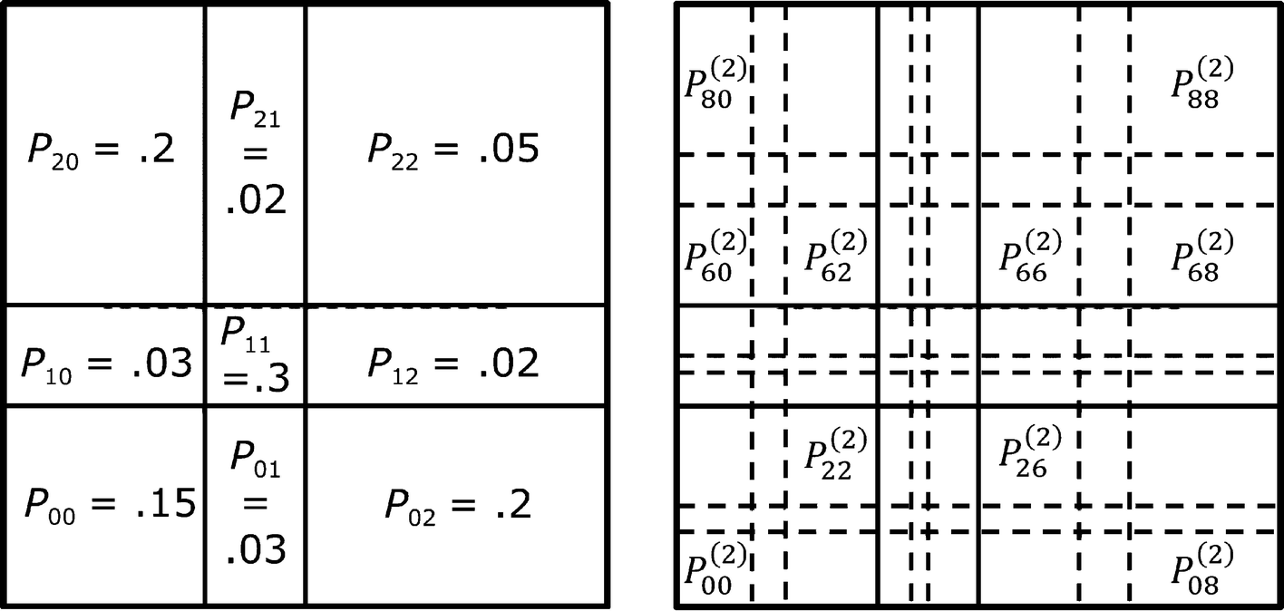
Generation-1 (left) and generation-2 (right) rectangles and their probabilities
 , then we slice R
ij vertically at a distance of
, then we slice R
ij vertically at a distance of  from the left-hand edge of R
ij and again at a distance of
from the left-hand edge of R
ij and again at a distance of  from the left-hand edge of R
ij. The horizontal slices of R
ij are similarly obtained from the V-slicing ratios and h. At the end of the generation 2 construction the original unit square [0, 1]2 has been subdivided into m
2 × m
2 rectangles, denoted by
from the left-hand edge of R
ij. The horizontal slices of R
ij are similarly obtained from the V-slicing ratios and h. At the end of the generation 2 construction the original unit square [0, 1]2 has been subdivided into m
2 × m
2 rectangles, denoted by  for i = 0, 1, 2, …, m
2 − 1 and j = 0, 1, 2, …, m
2 − 1. Let
for i = 0, 1, 2, …, m
2 − 1 and j = 0, 1, 2, …, m
2 − 1. Let  be the probability associated with
  . Figure 17.11 (right) illustrates the generation-2 construction, where for space considerations only some of the probabilities are indicated. For example, the rectangle R
20 with probability P
20 in Fig. 17.11 (left) is partitioned into 32 rectangles, whose probabilities are shown in Fig. 17.12.
. Figure 17.11 (right) illustrates the generation-2 construction, where for space considerations only some of the probabilities are indicated. For example, the rectangle R
20 with probability P
20 in Fig. 17.11 (left) is partitioned into 32 rectangles, whose probabilities are shown in Fig. 17.12.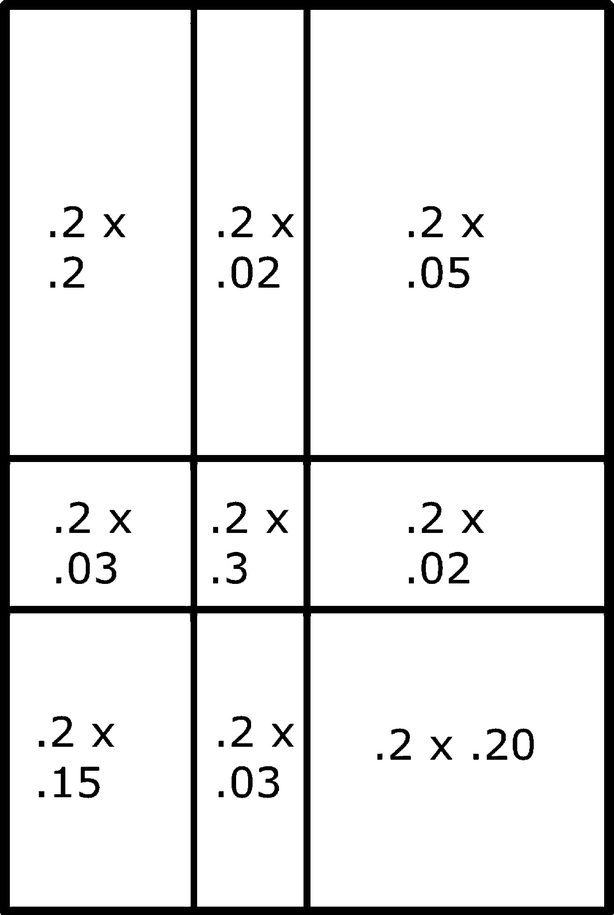
The second generation probabilities 
 be the probabilities after generation T. The formula for calculating these probabilities is [Horváth 13]

After calculating the probabilities  for a given set of H-slicing and V-slicing ratios, and for a given T, we are ready to generate the network. We follow the presentation in [Horváth 13] which assumed that the H-slicing ratios and the V-slicing ratios are the same. As illustrated in Fig. 17.11 (right), since the m
T rectangles
for a given set of H-slicing and V-slicing ratios, and for a given T, we are ready to generate the network. We follow the presentation in [Horváth 13] which assumed that the H-slicing ratios and the V-slicing ratios are the same. As illustrated in Fig. 17.11 (right), since the m
T rectangles  , j = 0, 1, ⋯ , m
T − 1 are adjacent to the bottom edge of [0, 1] × [0, 1] then the bottom edges of these m
T rectangles cover the interval [0, 1]. Let
, j = 0, 1, ⋯ , m
T − 1 are adjacent to the bottom edge of [0, 1] × [0, 1] then the bottom edges of these m
T rectangles cover the interval [0, 1]. Let  denote the set of nodes. For
  , generate a random number γ(n) from the uniform distribution on [0, 1]. Assume that the point
  lies in exactly one of the rectangles
  , j = 0, 1, ⋯ , m
T − 1. In the unlikely case that
, j = 0, 1, ⋯ , m
T − 1. In the unlikely case that  belongs to two rectangles, pick another random number for γ(n). Let β(n) be the index such that γ(n) lies in the rectangle
  . Since the indices i and j start at 0, then β(n) is between 0 and m
T − 1. (For example, for T = 1 and using the H-slicing and V-slicing ratios of
. Since the indices i and j start at 0, then β(n) is between 0 and m
T − 1. (For example, for T = 1 and using the H-slicing and V-slicing ratios of  , if for some
  we pick the random number γ(n) = 0.04, then β(n) = 0; if γ(n) = 0.4, then β(n) = 1; if γ(n) = 0.6, then β(n) = 2.) Performing this calculation for each node, we obtain β(n) for
  .
.
Consider the pair of nodes  and
and  . To determine if x and y will be connected, generate a random number p from the uniform distribution on [0, 1]. If
  we connect x and y by an undirected arc; otherwise, we do not connect x and y. Doing this for each pair of nodes generates the desired network. It is possible that this construction leaves some nodes isolated, and refinements to the method of [Palla 10] have been proposed [Palla 11] to eliminate this possibility.
 be the area of the rectangle whose probability is
  , the average node degree
〈δ〉 of the network is given by [Palla 10]
, the average node degree
〈δ〉 of the network is given by [Palla 10] 
 and from the normalization constraint on the probabilities we obtain 〈δ〉 = Nm
−2T. Thus, to keep 〈δ〉 constant as T increases, the number N of nodes must increase exponentially with T.
and from the normalization constraint on the probabilities we obtain 〈δ〉 = Nm
−2T. Thus, to keep 〈δ〉 constant as T increases, the number N of nodes must increase exponentially with T.Exercise 17.3 Implement this network construction, using the same H-slicing and V-slicing ratios. (The use of Python and C++ to implement this network construction was examined in [Horváth 13].) For various values of N, how do the fractal dimensions d B, d I, and d C vary as a function of T? □
The method can be modified so that the randomly generated network also exhibits a specified property, e.g., a desired degree distribution. This can be accomplished by using a simulated annealing approach, which attempts to minimize a suitably defined “energy” function. In simulated annealing, a small random change is made to the configuration, and the change is accepted if it lowers the energy. If the change increases the energy, the change is accepted with probability e −δ∕τ, where δ is the calculated increase in energy (δ > 0) and τ is a temperature which is gradually reduced. As applied to the multifractal network generator, the random change moves a rectangle boundary or changes one of the P ij values (if a change to some P ij value is accepted, then P ji must be changed by the same amount).
As the size of the networks generated by this construction increases, the networks become “topologically more structured” [Palla 10]. However, no claim was made in [Palla 10] or in [Horváth 13] that the networks constructed by this method actually exhibit multifractality. Yet this possibility was raised in [Palla 10], which suggested that this construction “is likely to result in networks displaying aspects of self-similarity in the spirit of the related findings” by [Song 05].
17.4 Computational Results for Multifractal Networks
In [Wang 11], Random Sequential Node Burning (Sect. 8.3) was applied to four classes of networks, to determine if multifractality is exhibited. Random (Erdős–Rényi), small-world,
scale-free,
and protein-protein
interaction (PPI) networks were analyzed. For each network studied, K executions of Random Sequential Node Burning were performed for each r value from 1 to Δ, for a total of KΔ executions; K = 200 was used in [Wang 11]. After the k-th execution of Random Sequential Node Burning has terminated for a given r, for q ≠ 1 the partition sum  was calculated; for q = 1 the partition sum is
  . Then, for each q, Z
q(k, r) was averaged over the K iterations, yielding
. Then, for each q, Z
q(k, r) was averaged over the K iterations, yielding  . For q ≠ 1, the estimate of D
q is 1∕(q − 1) times the slope, as determined by linear regression, of the
. For q ≠ 1, the estimate of D
q is 1∕(q − 1) times the slope, as determined by linear regression, of the  versus
  plot; for q = 1 the estimate of D
q is the slope of the Z
1(r) versus
plot; for q = 1 the estimate of D
q is the slope of the Z
1(r) versus  plot. To assess the extent to which the network is multifractal, define D
min ≡min−∞<q<∞D
q and D
max ≡max−∞<q<∞D
q. Then
plot. To assess the extent to which the network is multifractal, define D
min ≡min−∞<q<∞D
q and D
max ≡max−∞<q<∞D
q. Then  is multifractal if φ ≡ D
max − D
min is sufficiently large [Wang 11].
is multifractal if φ ≡ D
max − D
min is sufficiently large [Wang 11].
Erdős–Rényi random networks were generated by starting with N isolated nodes and connecting each pair of nodes with probability p. Since in general this can yield a disconnected network, the largest connected component (as determined by [Cytoscape]) was analyzed. For the nine networks studied, with N ranging from 449 to 5620, D max ∈ [2.42, 3.78], D min ∈ [2.14, 3.41], φ ∈ [0.28, 0.45], and there was no clear correlation between D q and N. The D q curve was found to be an increasing function of q for q < 0, and [Wang 11] cited other researchers who have observed, and offered explanations for, this “anomalous” behavior (this anomalous behavior was discussed in Sect. 17.2 above). From the φ values, [Wang 11] concluded that the multifractality of these networks is not clear-cut.
The small-world networks studied in [Wang 11] were generated using the Newman–Watts model [Newman 99b]. Let k be the desired node degree, where k is an even integer, and let p be a given probability. First, a regular ring lattice of N nodes was constructed: labeling the nodes n 0, n 1, …, n N−1, there is an undirected arc between nodes n i and n j if |i − j|≤ k∕2. For example, with N = 10 and k = 4, node n 5 is connected to nodes n 3, n 4, n 6, and n 7. Then each pair of nodes was connected with probability p; these are the shortcuts. For a set of eight networks with N = 5000, with k = 100, and with about 25, 000 arcs, both D min and D max were in the range [2.28, 3.08], and φ was in the narrow range [0.0, 0.06], so these networks were deemed not multifractal.
The scale-free networks studied in [Wang 11] were generated using an initial network of 5 nodes, to which nodes were added and arcs generated using preferential attachment (Sect. 2.4). Ten networks were generated with sizes ranging from 500 nodes and 499 arcs to 8000 nodes and 5999 arcs. The values of D min were in the range [1.36, 2.11], and D min generally (not always) increased with N. The values of D max were in the range [2.67, 3.39], and D max also generally increased with N. The values D min and D max increased with N since larger scale-free networks typically have more hubs which make the network structure more complex. The values of φ were in the range [1.22, 1.52], and there was no correlation of φ with N. The large values of φ, especially compared with D min, clearly indicated multifractality, which was the expected result, since in a scale-free network the density of arcs around the hubs is larger than the density of arcs elsewhere in the network.
Finally, the giant components of seven protein-protein interaction networks were analyzed in [Wang 11]. The data came from the [BioGRID] database of protein and genetic interactions, and from the Database of Interacting Proteins [DIP]. The giant components ranged in size from 1298 nodes and 2767 arcs to 8934 nodes and 41, 341 arcs. The values of D min were in the range [1.49, 2.87], and D min generally (not always) increased with N. The values of D min were achieved for q = 20. The values of D max were in the range [2.51, 4.89], and D max also generally increased with N. The D max values for these real-world networks were significantly higher than for the other three network classes examined in this study. The values of φ were in the range [0.89, 2.98], and there was no correlation of φ and N. The large values of φ, especially compared with D min, clearly indicated multifractality.
Exercise 17.4 ⋆ Is it possible to develop a statistically sound test that uses the D q values to determine whether a network should be classified as monofractal or multifractal? □
Exercise 17.5 Using the network construction method of [Li 14] (Sect. 12.1) with α = 0.1 and α = 0.8, plot D q for integer q ∈ [−10, 10]. □
17.5 Sandbox Method for Multifractal Networks
In Sect. 10.5, we introduced the sandbox method as a way of approximating the Grassberger–Procaccia algorithm for computing d
C of a collection of particles. The essence of the sandbox method is to determine the masses
of a set of boxes with radius r and with randomly selected centers, average the box masses for each r, and determine how the average mass scales with r. In Sect. 11.3, we showed that the cluster growing method for
computing the correlation dimension d
C of a network can be viewed as the sandbox method applied to a network. Then in Sect. 16.6 we presented the sandbox method for estimating the generalized dimensions D
q of a geometric object. The estimation is based on approximating the partition function value ∑j[p
j(s)]q (where the sum is over all non-empty boxes in the covering by boxes of size s) by the sum ![$$\sum _{n \in \widetilde {\mathbb {X}}} [M(n,r)/N]^{q-1}$$](../images/487758_1_En_17_Chapter/487758_1_En_17_Chapter_TeX_IEq282.png) , where the sum is over a set
, where the sum is over a set  of randomly chosen sandbox centers. The next logical step, to apply the sandbox method to calculate the generalized dimensions of unweighted networks, was taken by [Liu 15], and we now review those results.
 random nodes, but suggested that
  can depend on N. For q ≠ 1, define
 , [Liu 15] started with this definition of the sandbox dimension
of a geometric object:
, [Liu 15] started with this definition of the sandbox dimension
of a geometric object: ![$$\displaystyle \begin{aligned} {D_{q}^{\, \stackrel{ {\textit{sandbox}}}{}}} &\equiv \frac{1}{q-1} \lim_{r \rightarrow 0} \left\{ \log \left[ \frac{1}{\widetilde{N}} \sum_{n \in {\widetilde{\mathbb{X}}}} \left( \frac{M(n, r)}{N}\right)^{q-1} \right] \frac{1} {\log (r/\varDelta) } \right\} \\ &= \frac{1}{q-1} \lim_{r \rightarrow 0} \left\{ \left[ \log \frac{\textit{avg}\big( {M}_{q-1}(r) \big) }{N^{q-1}} \right] \frac{1} {\log (r/\varDelta) } \right\} \, . {} \end{aligned} $$](../images/487758_1_En_17_Chapter/487758_1_En_17_Chapter_TeX_Equ25.png)

 in [Liu 15] is 1∕(q − 1) times the slope of the
  versus
  plot over a range of r values, and linear regression was used to obtain this slope. The mass exponent τ(q) (Sect. 16.4) for q ≠ 1 was obtained using
  .
.In [Liu 15], the sandbox method was compared to compact box burning (Sect. 8.5) and to a variant of the box-counting method. First the comparison was made for three models of deterministic graphs, including (u, v)-flower networks (Sect. 12.2). For each of these models, the sandbox method CPU time was tiny compared to the other two methods. Plots in [Liu 15] showed that, for q ∈ [−10, 10], the three methods determined essentially identical estimates of τ(q) for each of the three network models. For all three network models, the plots of τ(q) versus q over the range q ∈ [−10, 10] were not quite linear, but rather were very slightly concave.
The sandbox method was also applied in [Liu 15] to three “real-world” network models. For scale-free
networks constructed using the Barabási–Albert preferential attachment model [Barabási 99],  ranged from about D
−10 ≈ 3.5 to D
10 ≈ 1.6 (although the
ranged from about D
−10 ≈ 3.5 to D
10 ≈ 1.6 (although the  versus q curves in [Liu 15] were characterized as convex, they do not appear to be convex for q ∈ [−10, 10]). For small-world
networks constructed using the Watts-Strogatz model [Newman 99b],
versus q curves in [Liu 15] were characterized as convex, they do not appear to be convex for q ∈ [−10, 10]). For small-world
networks constructed using the Watts-Strogatz model [Newman 99b],  decreased only slightly as q increased, with D
−10 ≈ 4.7 and D
10 ≈ 4.2 for N = 104. The conclusion in [Liu 15] was that multifractality of these small-world
networks is not obvious. Finally, Erdős–Rényi random networks
were constructed in which pairs of nodes were connected with small probabilities, and the largest connected component was analyzed. For these random networks, the
decreased only slightly as q increased, with D
−10 ≈ 4.7 and D
10 ≈ 4.2 for N = 104. The conclusion in [Liu 15] was that multifractality of these small-world
networks is not obvious. Finally, Erdős–Rényi random networks
were constructed in which pairs of nodes were connected with small probabilities, and the largest connected component was analyzed. For these random networks, the  versus q plot was a straight line with slope zero, so the networks are monofractal.
It was inevitable that the sandbox method would next be applied to multifractal weighted networks, and that step was taken in [Song 15], which also used (17.22) to calculate  .
The difference between the method of [Song 15] and the method of [Liu 15] described above is that whereas [Liu 15] used integer values of r, [Song 15] used possibly non-integer r values that are determined by the arc lengths. Let c
ij be the nonnegative length of the arc connecting nodes i and j, with c
ii = 0 for each i, and assume symmetric lengths (c
ij = c
ji). To determine the set of radius values to be used, order the arc lengths from smallest to largest. Represent these ordered A ≡ N(N − 1)∕2 arc lengths by
.
The difference between the method of [Song 15] and the method of [Liu 15] described above is that whereas [Liu 15] used integer values of r, [Song 15] used possibly non-integer r values that are determined by the arc lengths. Let c
ij be the nonnegative length of the arc connecting nodes i and j, with c
ii = 0 for each i, and assume symmetric lengths (c
ij = c
ji). To determine the set of radius values to be used, order the arc lengths from smallest to largest. Represent these ordered A ≡ N(N − 1)∕2 arc lengths by  , where
  for k
1 < k
2. Let K be the largest index such that K ≤ A and
for k
1 < k
2. Let K be the largest index such that K ≤ A and  , where Δ is the network diameter.
Then the radius values to be used are c
1, c
1 + c
2, …,
, where Δ is the network diameter.
Then the radius values to be used are c
1, c
1 + c
2, …,  . (A similar method for computing radii values was described in Sect. 8.2 on node coloring for weighted networks.) In [Song 15], using 1000 random sandbox centers and integer q ∈ [10, 10], linear regression was used to estimate
  for three large collaboration networks.
The sandbox method was applied in [Rendon 17] to a network of payments in Estonia. The nodes are companies, and there is an arc between two nodes if there was at least one transaction, in the year 2014, between the two companies. Multifractal analysis was performed on the skeleton  (Sect. 2.5) rather than on
  , since “by looking at the properties of the skeleton it is easier to appreciate the topological organization of the original network”.
The skeleton
, since “by looking at the properties of the skeleton it is easier to appreciate the topological organization of the original network”.
The skeleton  was computed using the arcs with the highest betweenness (Sect. 2.4);
the skeleton has diameter 34,
compared to Δ = 29 for
was computed using the arcs with the highest betweenness (Sect. 2.4);
the skeleton has diameter 34,
compared to Δ = 29 for  . The box counting dimensions of
  and
and  were nearly the same: 2.39 for
  and 2.32 for
  . The range of r used was 2–29, and the range of q was [−7, 12]. Since D
q ≈ 7.8 for q ∈ [−7, −4.5], at which point D
q decreased rapidly, and since minqD
q = 0.37, the conclusion in [Rendon 17] was that the network is multifractal.
. The range of r used was 2–29, and the range of q was [−7, 12]. Since D
q ≈ 7.8 for q ∈ [−7, −4.5], at which point D
q decreased rapidly, and since minqD
q = 0.37, the conclusion in [Rendon 17] was that the network is multifractal.
The sandbox method is not always successful: [Wang 11] found that the sandbox results did not yield a satisfactory fit for linear regression, and instead the results of Random Sequential Node Burning (Sect. 17.4) were averaged.
Exercise 17.6 In Sect. 16.6 we presented the barycentric variant of the sandbox method. Is there any way to adapt this method to a network? □
Exercise 17.7 In Sect. 16.6 we presented the recommendation in [Panico 95] that the calculations of the fractal dimension of an object should use measurements only from the interior of the object. Does this principle have applicability when calculating  for a growing network? □
Exercise 17.8 Does the fact that  and
and  have very similar box counting dimensions imply that the multifractal spectra of
  and
and  are very similar? Run some experiments to find out. □