2The branch structure of the Lambert W function

DOI: 10.1201/9781003168102-2

In the previous chapter, we mentioned several times that the Lambert function can take complex values. The equation xex=a is not solvable in the set of real numbers if a<−1/e (since xex has a global minimum at x=−1 with value −1/e), but it is solvable if we enable complex numbers to appear. If we do not restrict ourselves to the reals, a whole new world opens up. This chapter is dedicated to the thorough study of the complex Lambert function.

Before we start this study, however, it is instrumental to see everything on a simpler and more familiar function. We therefore first discover the behavior of the exp-log pair before going to see the xexp⁡ -W pair.

2.1 The exponential function

2.1.1 The mapping properties of exp

To know how the inverse of the exponential behaves, we need to see the mapping properties of exp. The exponential function is an entire function; its Taylor series

exp⁡(z)=∑n=0∞znn!

converges on the whole set ℂ to a finite value. It is also well known that

exp⁡(−z)=1exp⁡(z).

From these two facts, an important observation follows: exp⁡(z) can nowhere be zero. Indeed, if exp were zero in a point z0∈ℂ, then we would have that exp⁡(−z0)=1exp⁡(z0) is infinite, but we have just seen that exp takes finite values in all the points of the complex plane. Thus,

exp⁡:ℂ→ℂ*=ℂ∖{0}.

Picard's theorem says that a non-constant entire function can miss at most one value (see, for example, [110]). The exponential function, therefore, takes every complex number except zero. We are going to show that it takes every non-zero complex number infinitely many often.

Recall De Moivre's formula:

exp⁡(it)=cos⁡(t)+isin⁡(t) (t∈ℝ).

Therefore, |exp⁡(it)|=cos⁡2(t)+sin⁡2(t)=1, and the image of the imaginary axis by exp is the unit circle, spanned infinitely many times. Now analyze the more general expression with z=s+it:

exp⁡(z)=exp⁡(s+it)=exp⁡(s)exp⁡(it)=exp⁡(s)[cos⁡(t)+isin⁡(t)].(2.1)

The vertical axis with abscissa s is mapped onto the circle with radius exp⁡(s) (and with center in the origin¹), countably infinitely many times. This already shows our claim: every non-zero complex point is taken by exp infinitely many times.

Another proof

Recall the Great Picard Theorem: if an analytic function has an essential singularity at a point z, then in any neighborhood around z, the function takes every value with at most one exception infinitely often.

It is an immediate corollary of this theorem that a non-polynomial entire function takes every value with at most one exception infinitely many times. Indeed, if f(z) is a non-polynomial analytic function, then f(1/z) has an essential singularity at 0. From the Great Picard Theorem, it now follows that f(1/z) (and thus f itself) has the said property.

See [35] for the proof of the Great Picard Theorem.

2.2 The definition of the logarithm

After the acquaintance with the exponential, we can introduce its inverse. We have just seen that every point on the complex plane has infinitely many pre-images:

|exp⁡−1(w)|=|{z∈ℂ:exp⁡(z)=w}|=ℵ0 (w∈ℂ*).

If we want to know which z points are mapped to w(≠0) by exp, we recall (2.1) and calculate the radius of the circle which goes through w (this is simply |w|), and the angle of w. The logarithm of the radius, i.e., log⁡|w| will be ℜ(z). Here there is no problem, the positive real number |w| has a unique real logarithm.

_______________________

¹In this section, if no otherwise said, the circles are always centered at the origin.

The angle of w will be the imaginary part of z, but here we must be careful. Since

exp⁡(it)=cos⁡(t)+isin⁡(t)=cos⁡(t+2kπ)+isin⁡(t+2kπ)=exp⁡(i(t+2kπ)),

so the imaginary part of the pre-image z is determined only up to modulo 2π.

To proceed, we recall the argument functionarg which gives the angle of w such that it falls in the interval ]−π,π]. One could think that it would be of more sense to have the values on [0,2π[ ; but in this case, when we go around a circle of some positive radius, we will have a jump in the values of the arg function at the positive axis when we reach it from below (2π to zero) or from above (0 to 2π). Since this jump is inevitable if we want the arg function to take a unique value, it is preferred to have this jump on the negative real axis. This is also dictated by the long tradition.

It is thus seen that all those z's will constitute the pre-image of w for which ℜ(z)=log⁡|w|, and ℑ(z)=arg⁡(w)+2kπ (k∈ℤ). Hence, if w≠0, the pre-image of w is a set:

exp⁡−1(w)={z∈ℂ:z=log⁡|w|+i(arg⁡(w)+2kπ), k∈ℤ}.(2.2)

The value exp⁡−1(0) is not defined². The inverse of the exponential function, the logarithm, as we now see, is not a function but an infinite set of functions: for all integer k there is a well defined inverse of exp. These are the branches of the logarithm:

log⁡k(w)=log⁡|w|+i(arg⁡(w)+2kπ) (w∈ℂ*, k∈ℤ).(2.3)

Their ranges are horizontal strips of height 2π (see Figure 4):

log⁡k:ℂ*→{z∈ℂ:ℜ(z)∈ℝ, ℑ(z)∈ ]−π+2kπ,π+2kπ]}.

FIGURE 4 The range of the branches of the logarithm. The thick horizontal lines limit the ranges, and the dashed lines show the branch closure. For example, the range of the principal branch (−π<ℜ(z)≤π) does not contain the horizontal line at −π, so we draw a dashed line inside the range, right above the horizontal line at −π. In turn, the horizontal line at π does belong to the principal branch. These come from the definition of the arg function. The points A and B will be explained in Subsection 2.3.2.

The sub-index k is not the base of the logarithm, but a branch index. (We will not use logarithm of base different from e, so there will be no confusion.) The logarithm with which we met in high school is the branch with k=0, and it is the principal branch, denoted usually by log, without index:

log⁡(w)=log⁡|w|+iarg⁡(w) (w∈ℂ*).

This is the only branch which takes real values. Usually, the branch which has the (preferably positive) reals in its domain, or at least “the most of it” is the principal branch. Compare this with with the principal branch W₀ of the logarithm function.

_______________________

²The point w=0 does not belong to the range of exp. We naively could think that by defining exp⁡−1(0) in a suitable way, we could remedy this problem. This should be done such that log becomes continuous. This is impossible, as it turns out to be obvious after scrutinizing the logarithm more profoundly, see Subsection 2.3.2.

2.3 Branch cuts, covering maps, and Riemann surfaces

To prepare for the analysis of the branch structure of the Lambert function, we introduce some notions which facilitate talking about mappings and their inverses.

2.3.1 The z-plane and the w-plane

When considering equations like

exp⁡(z)=w and z=log⁡(w),

it is beneficial to distinguish between the z-plane and the w-plane. This makes the references easier and avoids confusion. In this case, the z-plane is the domain of exp; this plane is mapped to the w-plane by the same function. Set theoretically,

the z-plane is ℂ, and the w-plane is ℂ*.

In turn, log, the inverse of exp, maps the w-plane back to the z-plane. This is shown schematically in Figure 5.

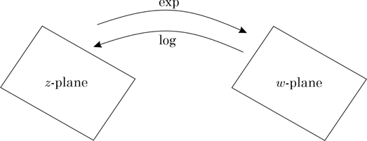
FIGURE 5 The exponential function maps the z-plane into the w-plane, the logarithm maps the latter into the former.

Thus, Figure 4 shows the z-plane, partitioned by the ranges of log. All of the individual horizontal strips are mapped by exp to the whole ℂ^*, and ℂ^* is mapped onto the horizontal strips by the corresponding branches of log.

2.3.2 Branch cut and branch point

It is useful to get a deeper insight into what happens with the lines limiting the horizontal strips of Figure 4 in the z-plane when mapped by exp. We saw earlier that horizontal lines are mapped into half-lines from the origin in the w-plane with angles determined by the ordinate of the line. The ordinates limiting the branches are the odd integer multiples of π by an odd integer, so these lines are all mapped onto the negative real axis. The negative axis in the w-plane has therefore a distinguished role. We have a name for it: the negative real axis is the branch cut of the logarithm; it is the set in the w-plane corresponding to the branch limiting lines in the z-plane.

If a horizontal line L in the z-plane is parametrized by s+i(π+2kπ) (k∈ℤ fixed, s∈ℝ), then

exp⁡(L)={−es:−∞<s<∞}.

The limiting point, when s→−∞, is the origin, the other one (when s→∞) does not belong to the finite plane. The origin is also the limiting point of the branch cuts. Because of this special role, the origin is the branch point of the logarithm.

Let us consider a circle going around the origin in the w-plane, as shown in Figure 6. This circle is the image of the vertical line segment A-B in the z-plane (and also the image of any line segments arising by shifting A-B up or down by 2π), as seen in Figure 4. The interiors of the segment A-B and the point B belong to the principal branch, but the point A does not. When traversing on the segment A-B on the z-plane, the exponential runs on the circle counter-clockwise in the w-plane. The images of the points A and B fall onto the branch cut. By the closure of the principal branch of the logarithm, the circle is continuous at its endpoint, exp(B). The branch cuts are usually chosen in such a way that this counter-clockwise continuity (CCC) holds.

FIGURE 6 Illustration of the branch cut. The meaning of the points exp(A) and exp(B) are detailed in the text.

Regardless of the radius of the circle, it always meets three branches (the principal branch, and log⁡±1). More generally, regardless of what kind of curve we use to connect two arbitrary points on the horizontal lines bounding the principal branch (or any other branch) in the z-plane, the image of this curve by the exponential always encircles the origin in the w-plane in counter-clockwise direction, see Figure 7.

FIGURE 7 The slanted line in the z-plane is mapped by the exponential to a spiral. The initial point of the spiral is exp⁡(A)=−e−3 and its enpoint is exp⁡(B)=−e3. Passing through the slanted line upward, the distance of the image point by exp grows, while its argument goes from −π to π.

2.4 Riemann surfaces

2.4.1 Motivation

It is an inconvenience that the logarithm and the Lambert function (and, in general, the multi-valued functions, such as z, arcsin, etc.) need a branch index to specify which concrete value we are talking about. Another problem is that complications might arise when we try to use “identities”, like

log⁡(xy)=log⁡x+log⁡y.

This equation indeed holds for positive real x and y, but not in general. Take, for example, x=y=−i. Then (do not forget that log without index denotes the principal branch)

log⁡(xy)=log⁡((−i)2)=log⁡(−1)=log⁡|−1|+iarg⁡(−1)=iπ.

On the other hand,

log⁡(x)+log⁡(y)=2log⁡(−i)=2(log⁡|−i|+iarg⁡(−i))=2i−π2=−iπ.

These problems motivated Bernhard Riemann to lay down a theory for the better understanding of multi-valued functions. His efforts culminated in a 1851 doctoral thesis, Foundations for a General Theory of Functions of a Complex Variable. Hermann Weyl further developed Riemann's ideas, and defined the abstract Riemann surfaces in his 1913 book The Concept of a Riemann Surface. Weyl wrote [183]:

I shared his [Felix Klein's] conviction that Riemann surfaces are not merely a device for visualizing the many-valuedness of analytic functions, but rather an indispensable essential component of the theory; not a supplement, more or less artificially distilled from the functions, but their native land, the only soil in which the functions grow and thrive.

All of these serve as a very good motivation for us to take a look at the general definition of Riemann surfaces, and apply what we have learned to the logarithm first, and then to the Lambert function. We will see that both of these functions can be represented as a single-valued function, by some “gluing process”. Riemann's idea was the following. Instead of taking much care about the range of multi-valued functions (log⁡−1 maps ℂ^* to the horizontal strip with imaginary part in ]−3π,−π], etc.), one could extend the domain of the function. If, in place of ℂ^*, we take an infinite copy of this set, the new single-valued logarithm will have enough space to map from this infinite copy to the whole ℂ, not only to the horizontal strips. Of course, if we want this new function to be continuous, we need some connection between the copies of ℂ^*, i.e., we need to “glue” these copies together in a meaningful way. The natural framework for all of this is the theory of Riemann surfaces and coverings.

2.4.2 Covering maps

We start with the formal definition of covering maps and the related notions, then we apply these to the exponential function and its inverse.

Let X and S be two topological spaces. The covering map is a continuous and surjective function p:S→X with the following property. For every x∈X there is an open (connected) neighbor U⊂X containing x, such that p−1(U) is a union of disjoint, open sets, the sheets in S, and these sheets are mapped homeomorphically onto U by p. X is the base space, and S is the total space of the covering in question. The pre-image p−1({x}) of x∈X by the inverse of p is a discrete subset of the total space S. Such sets are called fibers. The situation (without fibers) is depicted in Figure 8.

FIGURE 8 Illustration of a covering: p is the covering map, X is the base space, and S is the total space. The pre-image of U by p is a collection of disjoint subsets in S, which are called “sheets”.

2.4.3 The notion of a surface

The topological space S will be called surface, if it is a Hausdorff space, and every point s∈S has an open neighborhood homeomorphic to the open unit disk of ℂ. This latter requirement says that the surface S locally looks like a part of the complex plane. (That we denoted the total space and a generic surface with the same letter is not a coincidence. In our setting, these will indeed coincide.)

The definition of a Riemann surface is necessarily more complicated, because it introduces coordinate charts on (a family of open sets of) the surface, and requires that these charts satisfy some natural properties. We will not need these details later, so we do not go into details here (but we will still call our constructed surfaces Riemann surfaces, because this is the common reference in the literature, see, for example [42]). Instead, we show two simple examples of a Riemann surface. Certainly the simplest is the complex plane itself. A second example is the torus, where the unit square's two opposite sides are glued together such that first we have a “tube” of length one, then we glue the two ends of the tube. The torus clearly satisfies the requirements of a surface.

Next, we see the more complicated example of the Riemann surface of the logarithm. For the sake of better understanding, we first show a heuristic argument.

2.4.4 The Riemann surface of the logarithm – heuristic way

In high school we learned that the inverse of a function can be depicted by mirroring the graph of the function through the 45-degree line y=x. (See Figure 9).

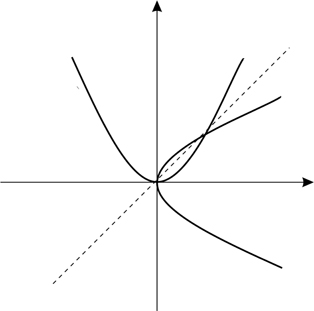
FIGURE 9 The graphical connection between the function f(x)=x2, and its inverse. The inverse of the upward function is drawn by mirroring the points of the original function through the dashed line y=x.

If we use this technique, from the graph of xex (Figure 1) we get the graph of W−1 and W₀ (Figure 2).

We want to extend somehow this technique to the complex plane. If we scrutinize this trick of mirroring, we realize that what we do is the interchange of the axes: y=f(x) means that we map the value of f at x above or below x, and, after mirroring we put the values of f on the x-axis, while the value(s) of the inverse will be drawn over and above the given point. We can do this with complex numbers also, but the problem is that we need four dimensions to do this. Indeed, let w=exp⁡(z) with z=s+it, and w=u+iv. We have four real parameters, s,i,u,v. With the aid of a computer, we can render three-dimensional images, and the value in the fourth dimension will be encoded in a gray value.

That is, on our graph, the horizontal (w-)plane is

ξ=ℜ(w)=ℜ(exp⁡(z))=exp⁡(s)cos⁡(t), andη=ℑ(w)=ℑ(exp⁡(z))=exp⁡(s)sin⁡(t).

We introduced ξ and η to make the computer coding easier. Over this plane we want to place the values of the logarithm, the z=s+it elements. As we cannot directly visualize two dimensions over a plane, we have two choices: (1) the real values (variable s) of log will go on the vertical axis, and we encode the imaginary values (t-values) with shades of gray, or (2) the imaginary values will go on the vertical axis, and we encode the real values with shades of gray.

After a moment of thinking, we realize that the first option would not visually work: all the branches have the same real part, (see (2.3)), while every branch has its own imaginary part, different from all the others. This would mean that over every point in the w-plane ((ξ,η) -computer plane) we would have a single point (the unique real part), but this point would have infinitely many different colors (a separate gray value for each of the imaginary parts). We therefore choose option 2.

On the language of computers, we take therefore the three-dimensional (ξ,η,ζ) -space, ξ and η will be given as above, we set ζ to be t, and then color this point with a gray value based on s. We choose the gray value such that the smaller the value of s, the darker the gray value.

With the computer package Mathematica we can do the above by typing in the command

c:=5ParametricPlot3D[{exp⁡(s)cos⁡(t),exp⁡(s)sin⁡(t),t},{t,−4π,4π},{s,−c,c},ColorFunction→Function{ξ,η,ζ,t,s},GrayLevelAbs[s]c,ColorFunctionScaling→False]

The ParametricPlot3D command plots a three dimensional surface in the (ξ,η,ζ) -space (Mathematica uses the x, y, and z symbols, but z denotes something else in our context). The points are determined by the first three values in curly brackets, then come the two parameters for the surface (here t and s). The next parameter gives how the surface is colored. The color is now determined by the absolute value of s. By setting the ColorFunctionScaling option to false, we tell Mathematica that we do not want the colors rescaled (to lie between 0 and 1); instead, we use the colors exactly as specified.

The execution of the command results in the plot that is given in Figure 10.

FIGURE 10 The Riemann surface of the logarithm. The arrow points to a line which belongs to the classical, real logarithm function whose values are pictured with gray values. Going toward the origin, the colors on the line are darker, meaning that log takes large negative values there. The lighter the color, the geater the value of the logarithm. In particular, the gray “loarithmically fades out” going outward of the origin, and it becomes white at infinite.

The spiral shape is due to the arg function. Going up/down in the ζ computer-coordinate, the argument function linearly increases/decreases. Revolving 360 degree (2π radius) around the origin, we make a period on the spiral.

The arrow points to the horizontal line which belongs to the principal branch over the line η=0 (as it is seen in the bottom). When the computer coordinate η is zero, we have sin⁡(t)=0, and t=0 in the principal branch. This horizontal line therefore encodes the “high school”-logarithm function. Going outward from the center of the plot, the points of the line are colored with gradually brighter gray values, signaling that the real part of the logarithm increases there. We see now that the high-school log function is just a tiny part of a big picture!

This surface revolves around zero in the t-coordinate (computer ζ) infinitely many times, it is continuous outside of the origin, and establishes a one-to-one connection between the punctured complex plane and the different branches of the logarithm function. This surface is the Riemann surface of the logarithm.

2.4.5 The Riemann surface of the logarithm – exact way

As we said above, we want to extend the domain of the logarithm so that the domain has “sufficiently many” elements to map continuously and bijectively to the whole complex plane, not only to the horizontal strips. It is natural to think that a covering map will help here, since the inverse of a covering map “multiplies” the base set. We therefore attempt to construct this domain extension of ℂ^* with the aid of coverings.

Let the base space be X=ℂ*, and let the total space S be a surface. Since S intents to be the extended domain of log, we want S to be mapped by a function L to the whole set ℂ (the union of the ranges of the branches of log) such that the image of each sheet of S by L corresponds to the image of a particular branch of the logarithm (a horizontal strip in ℂ). This aim can be reached via the covering map p:S→ℂ*. Our aim is equivalent with requiring the following. Let S be mapped by L onto ℂ and the images of L be further mapped by exp to elements in ℂ^* exactly as the covering p maps the points of Sdirectly onto ℂ^*. In short,

exp⁡°L=p.(2.4)

The relationship among S, ℂ^* and ℂ and their maps is shown in Figure 11. The requirement (2.4) can be expressed in algebraic terms: (2.4) is equivalent to the commutativity of the diagram of Figure 11, we require this diagram (without the log arrow!) to be commutative.

FIGURE 11 S is the Riemann surface of the logarithm, L is the continuous, single-valued logarithm, p is the covering which maps the Riemann surface S to ℂ^*. We require that exp⁡°L=p, as it is detailed in the text.

How should the surface S be imagined? The inverse of the covering p maps every point in ℂ^* back to S with infinite multiplicity. This shows that S should be considered as an infinite copy of the topological space ℂ^*. Indeed, if at the end of the day we want everything single-valued, these copies must be distinguishable. On the other hand, we want S not only to be a topological space as the notion of covering minimally requires, but we want it to be a surface, so S must locally be homeomorphic to ℂ. These altogether show that S must be taken as an infinite copy of ℂ^*.

We can make the situation more concrete by appealing to the requirement (2.4). Since p is continuous, L continuously maps the constituting copies of S onto the strips. As these strips join via horizontal lines, the copies of ℂ^* in S must also be joined. The horizontal lines correspond to the negative axis (branch cut) in ℂ^*, so we glue the copies of ℂ^* via these branch cuts (hence the name actually).

The cutting and gluing is as follows. We cut up the plane ℂ^* as it is shown on Figure 12. Let this plane be P₀. Next, we took another copy P₁ cut the same way, place it above P₀, and glue P₁'s dashed half-line to the solid line of the sheet P₀. Now take another copy, P−1, place it below P₀, and glue the open half-line of P₀ to the solid line of the sheet P−1. Continue this process upward and downward ad infinitum. This will be the Riemann surface S of the logarithm. As it is seen, it is the same as the plane we constructed heuristically in the previous subsection.

FIGURE 12 S is constituted by an infinite copy of the punctured plane ℂ^*. Each plane is cut as it is shown here. The dashed line does not belong to the set.

2.4.6 The monodromy group of the Riemann surface of the logarithm

Figures 4 and 6 and the text around them explained that a circle around the origin in the w-plane is mapped by a given branch of log such that we go through the whole strip belonging to this branch (see the A-B line segment in Figure 4). If we traverse the circle once again in the w-plane, we get the very same situation.

Now that we are familiar with the Riemann surface of the logarithm, let us see how the situation changes when we want to draw a circle around the origin. A short gaze at Figure 12 shows that the start and endpoint of the circle moved apart from each other. It is not a circle anymore but a curve: a spiral. If we wish, we can continue on this spiral upward or downward, stepping into another sheet of ℂ^*.

Notice that even to start to draw the curve, we have to specify which sheet we choose, because there are infinitely many of them. We had no such option on the single space ℂ^*.

As this is happening in the domain of the one-valued logarithm L, the logarithm of such a curve is passing through neighboring branches of the classical logarithm.

There are multi-valued functions for which the branches are taken in complicated orders when going around the branch points on a continuous curve. One can attach a group structure to the surface and to a fixed branch point which captures these branch-orders via permutations. This group of the surface is its monodromy group.

The Riemann surface of the logarithm has only one branch point, so there will be one single monodromy we want to determine. As we have already observed, going on our curve around the branch point zero, we touch the branches (which are indexed by the integers) in succession. Therefore, the monodromy group of the Riemann surface of the logarithm is the infinite cyclic groupZ.

2.5 The branches of the Lambert function

After seeing the simpler example of the logarithm, we are now ready to consider the branch structure of the Lambert W function.

2.5.1 The partition of the z-plane

The function zexp⁡(z) has a more complicated behavior than exp⁡(z) has. To see this, let z=s+it, and w=zexp⁡(z). Then

ℜ(w)=es(scos⁡t−tsin⁡t),(2.5)

ℑ(w)=es(ssin⁡t+tcos⁡t).(2.6)

While exp⁡(s+it)=exp⁡(s)exp⁡(it) was periodic in t with period 2π, w is not. Then how to proceed? We can do the reverse of what we did in the case of the logarithm. There we first realized that horizontal lines of distance 2π are mapped to the same half-line by exp, and we selected the half-line with −π angle (for matching with the tradition and with the usual definition of the arg function). Now let us see how the negative real axis is mapped by the Lambert function. If they partition the range of W, we are doing fine.

The complex number w falls onto the negative real axis if ℑ(w)=0, and ℜ(w)<0. The first requirement, by (2.6), means that

t=0, or ssin⁡t+tcos⁡t=0 (⇔ s=−tcot⁡(t)).(2.7)

The inequality ℜ(w)<0 is equivalent with

scos⁡t<tsin⁡t.

The equations in (2.7) are actually sufficient. If we draw the parametric curves encoded in (2.7), we see the plot on Figure 13: we have a partition of the complex plane by these curves.

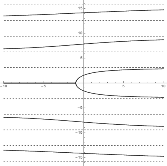
FIGURE 13 The partition of the z-plane by the images of the negative real axis in the range of the Lambert function (i.e., the inverse images of the negative real axis by z↦zexp⁡(z)). The dashed horizontal lines have their ordinate at non-zero multiples of π. The thick curves are asymptotic to these.

We therefore have the visual information, how the set

{W(u+iv):u<0, v=0}

partitions the z-plane. This suggests that our choice of making the negative real line to be the branch cut is (almost) correct. Why only “almost” will be seen in the next subsection.

2.5.2 The branch separating curves

The straight line separating W−1 and W1

If t=0, the situation is special. In this case ℜ(w)=ses, and we previously made the restriction ℜ(w)<0. This is satisfied when s<0. But then the line segment −1≤s<0 will belong entirely to the principal branch (see Figure 13, where already the correct separation is shown). Therefore, we must refine our idea a bit, and we have to choose not the whole negative real line, only the part for which s≤−1. This line separates the W−1 and W₁ branches. In the w-plane, this corresponds to the branch cut ℝ∋w<(−1)e−1=−1/e. A branch point in the domain of W is therefore w=−1/e. These belong to W−1, and W₀.

The other curves

The curves limiting the branches are more complicated than the simple horizontal lines of the logarithm, but their asymptotic behavior is easy to find. For these curves (if t≠0) it holds that

s=−tcos⁡(t)sin⁡(t)=−tcot⁡(t).(2.8)

When s tends to plus or minus infinity, then t must tend to the non-zero multiples of π from the corresponding direction.

The principal branch is limited by the curve

{−tcot⁡(t)+it:−π<t<π}.

(Notice that −tcot⁡(t) has only a removable singularity at t=0, where the limit is −1.)

The other curves are

{−tcot⁡(t)+it:2kπ<±t<(2k+1)π} (k=1,2,…).

These all correspond to the negative real axis in the domain of W, so the negative real line is another branch cut for the Lambert function; and the origin is thus a branch point.

It is now seen that W has two branch cuts: the negative real line, which belongs to infinitely many branches, and the half-line w<−1/e which belongs to W−1, and W₀. The corresponding branch points are the origin, and −1/e, respectively.

These curves form a part of a class of curves studied around 2500 years ago, and they are called trisectrix of Hippias or quadratrix of Dinostratus.

2.5.3 The trisectrix of Hippias

The invention of the trisectrix is attributed to Hippias of Elis (5th century BCE), who used it to solve the angle trisection problem (hence the name trisectrix). About 70 years later, Dinostratus (390-320 BCE) used the same curve in the study of the problem of squaring the circle. This explains why the curve is also called quadratrix.

Both the angle trisection problem and squaring the circle is an impossible task if one only uses ruler and compass. However, if the quadratrix is at our disposal (that is, we have a quadratrix template or a quadratrix compass), both problems become solvable.

The description of the curve is as follows. Consider a square ABCD as depicted in Figure 14, and draw an inner circle with center A connecting the points B and D. Now take a point E which travels with constant angular velocity on the circle; and take another point F which travels with constant velocity from point D downward to point A. The points E and F start moving from D at the same time instant, and the velocities are chosen such that the points will arrive at B and at A at the same time. The trisectrix/quadratrix is defined to be the set of points S which are the intersections of the horizontal line through F and the line segment AE¯.

FIGURE 14 The construction of the quadratrix.

The quadratrix can be drawn by using the tool depicted in Figure 15.

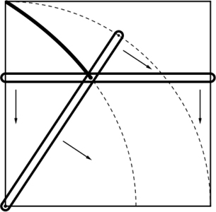
FIGURE 15 The quadratrix compass.

It is clear from the construction how to trisect an angle, or even more generally how to construct the angle α/n if α is a fixed angle and n≥2. The traversed vertical line segment by the point F is proportional to the traversed arc by the point E, thus dividing the line segment into n equal parts (between A and F) we divide the angle ∠EAB into n equal parts as well. The process for n=3 is drawn on Figure 16.

FIGURE 16 The solution of the angle trisection problem by using the trisectrix.

The quadratrix can be given by a one-parameter curve. Place the square ABCD on the Cartesian coordinate system such that A is placed at the origin, the vertex AB¯ on the x-axis. Supposing that the length of the vertices of the square is a, the quadratrix is given as

2aπ(tcot⁡(t),t), t∈]0,π2.

It is now apparent that the quadratrix indeed parametrizes the branch separating curves, see (2.8).

The three figures of this subsection were taken from WikiMedia Commons, see the article “Quadratrix of Hippias”. For more on the history, the reader is directed to [71].

2.5.4 The closure of the branches

We still have to sort out how the branches are closed. Remember that in the case of the logarithm, we used the counter-clockwise continuity (CCC) principle to decide where the branches of the logarithm will be closed and open; see Figures 4 and 6.

CCC will be applied for the branches of W as well. What we need to do is find out the images of circles by W, one around the branch point −1/e, and another around the other branch point 0.

The branch point at −1/e

A circle of radius r>0 around −1/e in the w-plane satisfies the equation

ℜ(w)+1e2+ℑ(w)2=r,

which, by (2.5)-(2.6), corresponds to the curve in the z-plane satisfying the equation

es(scos⁡t−tsin⁡t)+1e2+es(ssin⁡t+tcos⁡t)2=r.

Figure 17 shows this curve (where the radius is chosen to be one). By the CCC principle, the lower half of the limiting line therefore belongs to W−1 instead of W₀, while the upper half belongs to W₀. In other words, W₀ is “open from below” and “closed from above”: see Figures 19-20.

FIGURE 17 The image of a circle by the principal branch of the W function in the z-plane. By the CCC principle, the lower half of the branch limiting line therefore belongs to W−1, the upper half belongs to W₀.

The branch point at 0

A circle around the other branch point, 0, satisfies the equation

ℜ(w)+1e2+ℑ(w)2=r,

which, in the z-plane, gives the curve parametrized as

es(scos⁡t−tsin⁡t)2+es(ssin⁡t+tcos⁡t)2=r,

as it is seen on Figure 18. Since the curve goes upward, we infer by the CCC principle that the branches are open from below, and closed from above. See Figures 19, 20, and 21, respectively, for the branches W−1, W₀ and W₁.

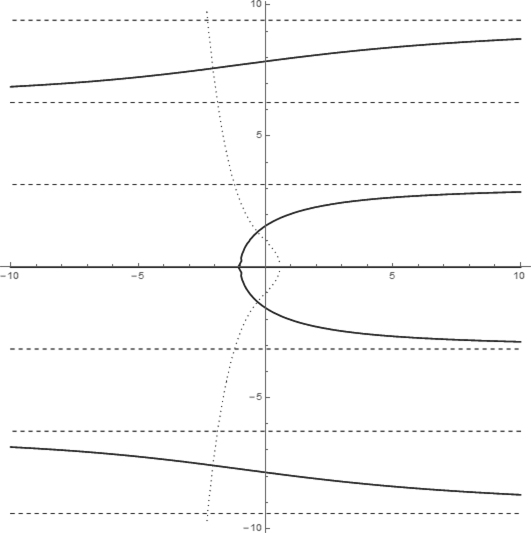
FIGURE 18 The image of a circle by the W function. By the CCC principle, the branches are open from below, and closed from above.

FIGURE 19 The closure of the branch W−1.

FIGURE 20 The closure of the branch W₀.

FIGURE 21 The closure of the branch W₁.

This choice of the closure is in agreement with our previous agreement that W−1 is the other branch having real values. If the branch closures were chosen differently, W₁ would have this feature.

2.5.5 The Riemann surface of the Lambert function

Now we study the Riemann surface and monodromies of the Lambert W function.

We number the sheets according to the branches they represent. Thus, for example, the zeroth sheet will belong to W₀, and so on. The ranges of the principal branch and that of W−1 meet along a curve; see Figure 13. This curve belongs to W−1, and it is the image of the interval [−∞,−1/e]. If we want this connection continuous, we must cut up the sheets of W₀ and W−1 along the interval [−∞,−1/e], and glue them together. Because of how the closures are fixed, the interval itself still belongs to the sheet of W−1 when glued to the same interval on the sheet of W₀. All of this is shown in the corresponding part of Figure 22.

FIGURE 22 Gluing of the sheets of the Riemann surface of W. L is the half-line of non-positive reals.

On the other hand, the sheet of W−1 still must somehow be glued to W−2 and W₁, because the ranges of these functions meet along curves. Let us deal with the connection of W−1 and W−2 first.

The curve along which W−1 and W−2 meet is the image of the negative real axis; therefore, we cut the −2 nd sheet along [−∞,0]. The −1 st sheet is already cut until [−∞,−1/e]. We cut up more this sheet, from ]−1/e,0]. Next, we glue these two half-lines of the two sheets such that the half-line [−∞,0] itself belongs to the −2 nd sheet (again, this is because of the closure choice we made earlier).

Next, we connect the sheets of W−1 and W₁. The branch cut on the −1 st sheet is almost entirely glued, only the interval ]−1/e,0] is left. But this is just how it should be, because W−1(]−1/e,0])=]−∞,−1[, the line along which W−1 and W₁ meet! We therefore glue the interval ]−1/e,0] on the two sheets in question. Note that this interval belongs to the −1 st sheet when glued.

The zeroth and first sheets must also be glued together, because there is a curve between the corresponding branches of W. This curve is W0(]−∞,−1/e[), so we take the interval ]−∞,−1/e[ on the two sheets and glue them together, such that the interval belongs to the zeroth sheet.

It is worth to check now the branch cuts of the first, zeroth, and minus first sheets: all of them have already been glued together in such a way that is consistent with the closures fixed previously by the CCC principle!

The rest is easy: we glue the branch cut of the −2 nd sheet to the cut made on the −3 rd sheet. By CCC, the interval belongs to the −3 rd sheet. We go downwards similarly. Next, the first sheet is glued along its cut to the second sheet; the interval itself belongs to the first sheet. We then glue the sheets above these in the same way.

Notice one peculiarity: the −1 st and first sheets are glued together, but this connection does not involve the zeroth sheet. This means that the Riemann surface of W cannot be drawn in the three-dimensional space without intersecting the zeroth sheet, because this latter is located “in between”. This intersection is only virtual, if we embed the surface in a four-dimensional space, it has no intersections. This virtual intersection can perfectly be seen if we use the technique of Subsection 2.4.4, and draw the Riemann surface of W on a computer screen. This is done in Figure 23.

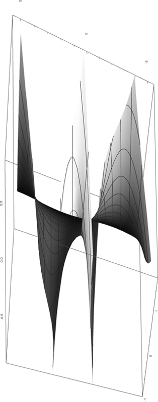
FIGURE 23 The Riemann surface of W.

The Mathematica code for plot 23 is the following:

ParametricPlot3D{exp⁡(s)(scos⁡(t)−tsin⁡(t)),exp⁡(s)(ssin⁡(t)+tcos⁡(t)),t},{t,−5,5},{s,−6,1},AspectRatio→0.4,ColorFunction→Function{x,y,z,t,s},GrayLevels+67,ColorFunctionScaling→False

2.5.6 Monodromies

After seeing how the sheets of the Riemann surface of W are glued together, we have no difficulty when determining the monodromy groups of the surface encircling the two branch points −1/e and 0.

Let us fix a circle of positive orientation around the origin of ℂ with radius <1/e, and with infinite winding number. This circle becomes an infinite open curve on the Riemann surface. Figure 22 shows us that if we follow the curve, it trespasses the sheets in this order:

…,−3,−2,−1,1,2,3,….

The zeroth sheet is not crossed at all. The monodromy group of the origin is the infinite cyclic group, ℤ.

Next, fix a circle around −1/e with radius <1/e and of positive orientation. Now the winding number can be finite, because only three sheets (with index ±1 and 0) will be involved. If we start on the zeroth sheet, we can easily follow the curve by following the way of gluing: −1/e will be encircled entirely on the zeroth sheet starting on the dashed line of Figure 22. Reaching the solid line, we jump up to the first sheet, and we make a half-circle around −1/e there, then we are led by the surface down to the minus first sheet, and make a half-circle there, too.

The monodromy group of the point −1/e is therefore the cyclic group of order three, C₃.

To get a better visual information of how circles are mapped by the different branches of the Lambert function, we refer to Figures 24-25.

FIGURE 24 The images of three circles around the origin by W. The dotted curves (notice the tiny dotted curve around the origin inside the image of W₀) belong to the circle of radius 1/e−0.2. The dashed curves belong to the circle of radius 1/e. The dotdashed curve is the image of the circle of radius 1/e+1.

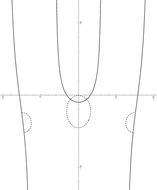
FIGURE 25 The images of three circles around −1/e by W. The radius of the circle is 1/e−0.05.

2.5.7 The fixed points of the Lambert function

The fixed points of the Lambert function are very easy to find, since these are the fixed points of its inverse zez, too. Since

zez=z, if and only if ez=1,

we see that

z=log⁡k(1)=log⁡|1|+i(arg⁡(1)+2kπ)=2kπi (k∈ℤ).

Thus W(2kπi)=2kπi, but still we need to know which branch must be taken for the different k values. Thanks to the information that we have just gained about the branches of the Lambert function, a simple visual inspection of Figure 13 tells us that the branch index coincides with k. We get that

Wk(2kπi)=2kπi (k∈ℤ).

Further notes

1. Coverings. The covering map is a very important notion in algebraic topology: it helps analyze the topological nature of the base space. It is also important in the study of algebraic curves. See more on this topic in [123].

2. Monodromy group. The definition of the monodromy group would require some preparation. The logarithm and even the Lambert function does not require such a heavy machinery, because their monodromy structure is very simple. So we do not need the exact definition of the monodromy group. The book [96] is suggested for those readers who would like to know more about the monodromy group in general. One can learn from this text, for example, that the monodromy group of 1+z is the dihedral group of order eight, a result which is not at all obvious.

3. Some mapping properties of W. By motivations coming from the analysis of delay differential equations, it was proven by Shinozaki [165] that ℜ(Wk(rejθ)) is a monotone increasing function of r for any fixed non-zero k (Lemma A.3). Another useful fact proven by Shinozaki is that, outside of the branch cuts,

   max⁡k∈ℤRe(Wk(z))=Re(W0(z)).