3Unwinding number, and branch differences. The functions K, ω, and M

DOI: 10.1201/9781003168102-3

In this chapter, we make precise some sloppy “symbolic” calculations of the first chapter. It turns out that identities like W(x)+log⁡W(x)=log⁡x (see (1.21)) are not true for arbitrary complex x, but some “correction terms” can be introduced such that the validity of these identities extends to the whole complex plane. This correction term is found via the so-called unwinding number K(z).

Second, it will be shown through an example, how to find all solutions of some equations from the first chapter. The Wright ω function, which is of independent interest, will be of great help in doing this.

In the last part of this chapter, we study the branch difference function Mm,n(z)=Wm(z)−Wn(z). This branch difference is motivated by the branch difference of the logarithm. But, while ln⁡n(z)−ln⁡m(z)=2π(n−m), the function Mm,n(z) is highly non-trivial and has some interesting properties.

3.1 Why does the complex version of many identities fail?

3.1.1 Non-identities regarding the logarithm

When solving logarithmic equations in high school, we frequently used identities like

log⁡(x2)=2log⁡x,

or

log⁡(xy)=log⁡x+log⁡y.

While these both are true when x and y are real, they fail to be true in general. Indeed, let us take x=−1 in the first displayed equation above. Then

log⁡((−1)2)=log⁡1=0,

but

2log⁡(−1)=2(log⁡|−1|+iarg⁡(−1))=2πi.(3.1)

This shows that the second identity also fails, because it is a generalized version of the first one; but it can be seen otherwise. Take x=−1, and y=i. Then

log⁡(xy)=log⁡(−i)=log⁡|−i|+iarg⁡(−i)=−π2i.

On the other hand (by making use of (3.1)),

log⁡(x)+log⁡(y)=log⁡(−1)+log⁡(i)=πi+log⁡|i|+iarg⁡(i)=πi+iπ2=3π2i.

What goes wrong? We can see it by carefully analyzing the proof of the non-identity log⁡(xy)=log⁡x+log⁡y. A possible proof is as follows. Start with xy=elog⁡xelog⁡y, then note that elog⁡xelog⁡y=elog⁡x+log⁡y. So far, everything is correct. Now take logarithm:

log⁡(xy)=log⁡elog⁡x+log⁡y=!log⁡x+log⁡y.

While it is true, that elog⁡x=x, it is not true, that log⁡(ex)=x, so the very last step is not correct¹. Indeed, there are infinitely many different values of the logarithm; we must specify which one we are taking. If the wrong branch is picked, we lose the validity of the identity.

It is therefore very useful to find the exact form of the difference z−log⁡(ez). We will do this later, but first we show that many other identities that seemingly have no relation to the logarithm go wrong when extending from the real line to the complex plane.

3.1.2 Non-identities regarding roots

We do not need to use the logarithm to see some confusing aspects of the “usual high school algebra” when extended to complex numbers.

It is seemingly okay to do the following calculation:

z−1z+1=(z−1)(z+1)=z2−1.(3.2)

Using this “identity”, we infer, by putting z=−2, that

−3−1=3.(3.3)

On the left-hand side, we might argue that

−3−1=−13−11=i23=−3.(3.4)

We have a sign mismatch here. Should we, instead, do the following?

−3−1=−13−11=(−1)(−1)3=3.(3.5)

_______________________

¹Take x=2πi: log⁡(e2πi)=log⁡(1)=0≠2πi. Instead, what is true is log⁡(e2πi)=log⁡1(1)=2πi, where log₁ is the k=1 branch of the logarithm.

This gives the answer which matches with (3.3). What is going on here? The problem is that at several points in the above calculations we used non-permitted branch choices. For example, if we had used −−1 (which is the other branch of the square root) in (3.5) in one and only one place, we would have gotten −3, as in (3.4).

If we want to do the calculations correctly, we must recall that, by definition,

z=exp⁡12log⁡z.

Here the principal branches are used for both the square root and the logarithm. Then

−3=exp⁡12log⁡(−3)=exp⁡12(log⁡3+iarg⁡(−3))=

exp⁡12log⁡3+πi2=exp⁡12log⁡3exp⁡πi2=

3exp⁡12log⁡(−1)=3−1=i3.

Thus −3−1=i23=−3≠3, which means that (3.2) is plainly incorrect. In general, it is false that z1z2=z1z2.

Again, we can see more closely where the problem appears by trying to do the proof:

z1z2=exp⁡12log⁡(z1z2)=!exp⁡12log⁡z1+12log⁡z2)=

exp⁡12log⁡z1exp⁡12log⁡z2=z1z2.

We saw in the last subsection that log⁡(z1z2)=log⁡z1+log⁡z2 does not always hold, and we also saw that this has something to do with the fact that log⁡(ez)≠z.

We therefore now start to study the function z−log⁡(ez).

3.2 The unwinding number

3.2.1 The definition of the unwinding number

It is not always true that z−log⁡(ez)=0, and this difference manifests itself when we try to extend identities from the positive real line to the complex plane (and even when extending identities to negative reals).

Let z=s+it, and do the following calculation (with respect to the principal branch of log):

z−log⁡(ez)=s+it−log⁡(es+it)=s+it−log⁡|es+it|+iarg⁡(es+it).

Notice that |es+it|=es, and thus log⁡|es+it|=log⁡|es|=log⁡es=s for positive real s. Moreover, arg⁡(es+it)=arg⁡(eit). Since the argument is in ]−π,π], t and arg⁡(eit) differs in an integer multiple of 2π: t=arg⁡(eit)+2kπ for some integer k. The above displayed line therefore gives that

z−log⁡(ez)=it−iarg⁡(eit)=

i(arg⁡(eit)+2kπ)−iarg⁡(eit)=2kπi.

Thus the difference between z and log⁡(ez) is an integer multiple of 2πi, which is not a surprise: this is the difference between the corresponding points on different branches of the logarithm.

Hence

k=z−log⁡(ez)2πi.

On the other hand, from the usual definition of the logarithm (see (2.3)) it is immediate that

k=ℑ(z)−π2π.

Indeed, notice that if −π<ℑ(z)≤π, then k=0, which means that z lies on the horizontal strip of the principal branch. If −3π<ℑ(z)≤−π, then k=−1, which again correctly gives that we are on the branch of log⁡−1. We therefore introduce the unwinding number as

K(z):ℂ→ℤ; K(z)=ℑ(z)−π2π.(3.6)

With this function we have the universally true expression

log⁡(ez)=z−2πiK(z) (z∈ℂ).(3.7)

The K(z) function (with a different sign) was introduced in the paper [41]. Later the authors noted [43] that calculations are easier (less minus signs appear) if K(z) is defined as we did here.

Let us see how the unwinding number corrects the wrong identities we dealt with previously.

3.2.2 The use of K(z)

Until the end of this chapter, we will not need the notion of w- and z-planes; the arguments will be denoted by z,z1,z2, as usual.

Correcting log⁡(z1z2)=log⁡z1+log⁡z2

The non-identity log⁡(z1z2)=log⁡z1+log⁡z2 can be corrected by the use of K(z). This is done as follows. We start with

z1z2=exp⁡(log⁡z1)exp⁡(log⁡z2)=exp⁡(log⁡z1+log⁡z2).

We should not be afraid; it is always true that exp⁡(z1)exp⁡(z2)=exp⁡(z1+z2). Now take (the principal branch of the) logarithm of both sides in the last displayed equation:

log⁡(z1z2)=log⁡exp⁡(log⁡z1+log⁡z2).

Here is the point where the unwinding number comes into the picture: the log of an exp must be corrected by K:

log⁡exp⁡(log⁡z1+log⁡z2)=log⁡z1+log⁡z2−2πiK(log⁡z1+log⁡z2),

whence

log⁡(z1z2)=log⁡z1+log⁡z2−2πiK(log⁡z1+log⁡z2).(3.8)

Applying this to our example on p. 71, we get that

log⁡(−i)=log⁡(−1)+log⁡(i)−2πiK(log⁡(−1)+log⁡(i))=

πi+π2i−2πiK3π2i=3π2i−2πi3π2−π2π=

3π2i−2πi14=3π2i−2πi=−π2i.

It can similarly be seen that

log⁡z1z2=log⁡z1−log⁡z2−2πiK(log⁡z1−log⁡z2),

in particular,

log⁡1z=−log⁡z−2πiK(−log⁡z).(3.9)

Correcting z1z2=z1z2

We saw that z1z2 does not always equal z1z2, because the two branches of the square root mix things up. Since the two branches of the square root only differ by a sign, we expect an occasional −1 factor multiplying z1z2.

The following chain of reasoning results in the correct answer:

z1z2=exp⁡12log⁡(z1z2)=

exp⁡12log⁡z1+12log⁡z2−2πi2K(log⁡z1+log⁡z2)=

exp⁡12log⁡z1exp⁡12log⁡z2exp⁡−πiK(log⁡z1+log⁡z2)=

z1z2exp⁡−πiK(log⁡z1+log⁡z2).

Since the unwinding number is integer, and exp⁡(−πik)=(−1)k, we get that

z1z2=z1z2(−1)K(log⁡z1+log⁡z2).

3.3 Corrected identities for the Lambert function

After seeing elementary examples which show that care must be taken when proving formulas with complex functions, we turn to the Lambert function. In the first chapter we saw numerous identities satisfied by W. While they are true for the principal branch at positive real argument (where everything is real and even positive), there are troubles when we try to extend those identities to other branches and complex arguments. In this section we clarify this issue, and the unwinding number will be very handy in doing so.

3.3.1 Correcting (1.21)

Before we start, let us prove a simple identity which will be needed:

K(z−2πin)=K(z)−n.(3.10)

By the definition (3.6),

K(z−2πin)=ℑ(z−2πin)−π2π=ℑ(z)−2πn−π2π=

ℑ(z)−π2π−n=K(z)−n.

To find the form of (1.21) which would be valid on the whole plane, we take the logarithm of Wk(w)eWk(w)=w correctly. Leaving the argument of W_k, we get from (3.8) that

log⁡Wk+log⁡eWk−2πiK(log⁡Wk+log⁡eWk)=log⁡w.

Now, applying (3.7) for the second term, we have that

log⁡Wk+Wk−2πiK(Wk)−2πiK(log⁡Wk+log⁡eWk)=log⁡w.(3.11)

The term log⁡eWk inside the unwinding number is expanded again with (3.7):

K(log⁡Wk+log⁡eWk)=K(log⁡Wk+Wk−2πiK(Wk)).

Since K(Wk) is an integer, we can use (3.10) to see that

K(log⁡Wk+Wk−2πiK(Wk))=K(log⁡Wk+Wk)−K(Wk).

With this, (3.11) simplifies to

log⁡Wk+Wk−2πiK(log⁡Wk+Wk)=log⁡w.(3.12)

It turns out that the unwinding number of log⁡Wk+Wk is a simple function of k:

K(log⁡W−1+W−1)=0,if −1e≤w<0;−1,otherwise,(3.13)

and if k≠1, then

K(logWk+Wk)=k(3.14)

Let us prove these identities.

Notice that ℑ(log⁡Wk)=arg⁡Wk, and thus

K(log⁡Wk+Wk)=arg⁡Wk+ℑ(Wk)−π2π.

This equals k when arg⁡Wk+ℑ(Wk)∈ ](2k−1)π,(2k+1)π]. Recall (2.5)-(2.6). Fix w=reiθ, with which equations (2.5)-(2.6) become

rcos⁡θ=es(scos⁡t−tsin⁡t),rsin⁡θ=es(ssin⁡t+tcos⁡t).

Divide the first equation by the second one (given that θ∈{0,π}):

cot⁡θ=cot⁡(arg⁡Wk)cot⁡t−1cot⁡(arg⁡Wk)+cot⁡t=cot⁡(arg⁡Wk+ℑ(Wk)).

These equalities hold for arbitrary r, and, in particular, also when r→∞. When w is large so that r is large but θ fixed (so we are moving on a ray R of the w-plane), w=zez must be large, and z must be large, too. But for large z, the exponential dominates, and the inversion of zez is therefore close to the logarithm. In other words, the Lambert function asymptotically behaves like the logarithm. Since the ray R is mapped to a horizontal line by the logarithm, and points on R with large magnitude are mapped to points with large positive real part but fixed imaginary part, we see that lim⁡r→∞arg⁡log⁡R=0, the same is true for the branches of the Lambert function:

lim⁡r→∞arg⁡Wk(reiθ)=0 (θ∈ ]−π,π[ ∖{0}).

Consequently,

lim⁡r→∞(arg⁡Wk+ℑ(Wk))=lim⁡r→∞ℑ(Wk)=

lim⁡r→∞t=θ+2kπ.

This is so, because the image of R by the branches of W_k approach the horizontal lines of log⁡(R) asymptotically, and ℑlog⁡k(R)=θ+2kπ. It now follows, that arg⁡Wk+ℑ(Wk)∈ ](2k−1)π,(2k+1)π], except at least when k=−1. This case needs special attention because if −1/e≤w<0, then W−1(w) is a negative real number, and

arg⁡W−1+ℑ(W−1)=arg⁡W−1=π,

so now K(log⁡W−1+W−1)=0, as stated.

Using (3.13)-(3.14) with (3.12), we get that

Wk(z)+log⁡Wk(z)=log⁡z,if k=−1,z is real,and −1/e≤z<0;log⁡z+2πik,otherwise.(3.15)

3.3.2 Correcting (1.23)

The neat formula (1.23) holds only for real values, but in this section we extend it to the whole complex plane. Our statement is the following.

For all a,b,z,w∈ℂ, and integer h, we have that

aWh(z)+bWh(w)=

Wk​​(aWh(z)​+​bWh(w))zWh(z)awWh(w)bexp⁡2πi[aK(Wh(z))​+​bK(Wh(w))]​​,

where the branch index k must be chosen as follows. Let g=aWh(z)+bWh(w), and f=−ℑ(g)cot⁡(ℑ(g)).

1. If ℑ(g)=0, and ℜ(g)≥−1 ⇒ k=0,

2. if ℑ(g)=0, and ℜ(g)<−1, ⇒ k=−1,

3. if 0<ℑ(g)<π, and ℜ(g)≥f ⇒ k=0,

4. if 0<ℑ(g)<π, and ℜ(g)<f ⇒ k=1,

5. if −π<ℑ(g)<0, and ℜ(g)≤f ⇒ k=−1,

6. if −π<ℑ(g)<0, and ℜ(g)>f ⇒ k=0,

7. if ℑ(g)=nπ with odd n>0, and ℜ(g)<+∞ ⇒ k=n+12, and if ℜ(g)=+∞ ⇒ k=n−12,

8. if ℑ(g)=nπ with even n>0 ⇒ k=n/2,

9. if ℑ(g)=nπ with even n<0, and ℜ(g)>−∞ ⇒ k=n/2,

10. if ℑ(g)=nπ with even n<0, and ℜ(g)=−∞ ⇒ k=n/2−1,

11. if ℑ(g)=nπ with odd n<0 ⇒ k=n−12.

    Moreover, if ℑ(g) is not a multiple of π, and it is in the complement of the interval [−π,π], then let n:=⌊ℑ⁡(g)/π⌋. Now,

12. if ℑ(g)>0, n is odd ⇒ k=n+12,

13. if ℑ(g)>0, n is even, and ℜ(g)<f ⇒ k=n/2+1,

14. if ℑ(g)>0, n is even, and ℜ(g)≥f ⇒ k=n/2,

15. if ℑ(g)<0, n is even ⇒ k=n/2,

16. if ℑ(g)<0, n is odd, and ℜ(g)≤f ⇒ k=n−12,

17. if ℑ(g)<0, n is odd, and ℜ(g)>f ⇒ k=n+12.

The proof

We look for an expression for aWh(z)+bWh(w), so we write

[aWh(z)+bWh(w)]eaWh(z)+bWh(w)=s(z,w,a,b,h)=:s.

The solution of this equation is, by definition, Wk(s) with a given branch index k, such that s falls into the image of Wk(s). This requirement will be dealt with later.

For the moment, we have that

Wk(s)=aWh(z)+bWh(w).(3.16)

We rewrite s as

s=[aWh(z)+bWh(w)]eaWh(z)+bWh(w)=

[aWh(z)+bWh(w)]eaWh(z)ebWh(w).

Recall that eWh(z)=z/Wh(z), and eWh(w)=w/Wh(w). In the next step, we elevate these to the powers a and b, respectively. Here we must be careful, since it does not hold true in general, that eba=(eb)a. Instead, what is true is

eba=(eb)ae2πiaK(a),

which is a particular case of the more general identity

zba=(zb)ae2πiaK(alog⁡z),

see [25].

Now we therefore have that

eaWh(z)=(eWh(z))ae2πiaK(Wh(z))=zWh(z)ae2πiaK(Wh(z)),

and, similarly,

ebWh(w)=wWh(w)be2πibK(Wh(w)).

Upon substituting these into the expression of s, we see that

s=[aWh(z)+bWh(w)]zWh(z)awWh(w)be2πi[aK(Wh(z))+bK(Wh(w))].

This and (3.16) yield the formula in our statement.

We still need to find the proper branch index k. Since the determination of k is elementary but laborious, we will consider only three particular, but representative, cases.

1. Let us suppose that g=aWh(z)+bWh(w) is real. The only branches which contain real values belong to the indices k=0 and k=−1. If k=0, the range of the function W₀ contains [−1,+∞[, and the range of W₁ contains ]−∞,−1]. Consequently, if ℜ(g)≥−1 we have that k=0, otherwise k=−1. This shows the first two particular cases in our theorem. (Note that if ℜ(g)=−1, we could equivalently choose k=−1.)

2. Next, let us suppose that ℑ(g) is a positive multiple of π. First, let n be odd. By inspecting Figure 13, we see that all the points ξ+nπi belong to the branch k=(n+1)/2 for finite ξ. However, because of the branch closure, of ξ=+∞, we are still on the branch (n−1)/2. If n is even, the whole extended horizontal line ξ+nπi is contained in the range of the branch indexed by n/2. These considerations cover the seventh and eighth cases in our theorem.

3. We now pick a case when ℑ(g) is positive, but it is not a multiple of π. If ℑ(g) is in the interval ]nπ,(n+1)π[ with even n (note that n=⌊ℑ⁡(g)/π⌋), then we have two possibilities: (1) ℑ(g) falls strictly on the left-hand side of the curve separating Wn/2 and Wn/2+1. The separating curve's real coordinate is −ℑ(g)cot⁡(ℑ(g))=:f, and thus falling on the left of this curve means that ℜ(g)<f; in which case k=n/2+1 (confirming the case 13). (2) ℑ(g)≥f. Since the curve itself, and the points with real coordinate greater than f all fall into the range of Wn/2, we get that k=n/2 (this is case 14). Now let ℑ(g) belong to the interval ]nπ,(n+1)π[ with odd n. Since all the finite points with such an imaginary coordinate belong to W(n+1)/2, we get that k=(n+1)/2. This is case 12 in our theorem.

The rest of the cases can be seen similarly.

Some neat examples

To see how the theorem is applied, we deduce several special values for the Lambert function.

For example, the following special value for W−1 is given:

W−1Ω−eΩee=Ω−e.

Choose a=1, b=−1, z=1, w=e·ee, and h=0. Then

aWh(z)+bWh(w)=W0(1)−W0(e·ee)=Ω−e.

Since Ω−e≈−2.15114, we get that k=−1 (see case 2), and our formula states that

Ω−e=W−1(Ω−e)1W0(1)e·eeW(e·ee)−1e2πi·0=

W−1(Ω−e)1Ωe·eee−1=W−1Ω−eΩee,

which confirms our result.

To see a complex special value, we present the following corollary.

W0iΩΩi=iΩ.

To see this, substitute a=b=i/2, z=w=1, h=0, such that

aWh(z)+bWh(w)=i2W0(1)+i2W0(1)=iΩ.

The branch index is given by using case 3: 0<ℑ(iΩ)=Ω<π, and

−ℑ(iΩ)cot⁡(ℑ(iΩ))=−Ωcot⁡(Ω)≈−0.89<ℜ(iΩ)=0,

so k=0, indeed. (Note that the presented identity is the particular case of (1.29), but that was proven only for real x values.)

Similarly,

W02iΩΩ2i=2iΩ,

but then a jump on the branch comes:

W13iΩΩ3i=3iΩ.

Indeed,

−ℑ(3iΩ)cot⁡(ℑ(3iΩ))=−3Ωcot⁡(3Ω)≈0.22>ℜ(3iΩ)=0,

thus k=1, as case 4 tells us.

3.4 The Wright ω function

3.4.1 Looking at equation x+log⁡x=a more carefully

The reader has seen a large number of examples on the previous pages where the usual high school algebra was shown to be failing. Suspicion therefore arises whether the solutions presented for the equations in Section 1.1 are indeed correct. If we are interested in real solutions (and this is the case in most of the applications), we can still do the usual algebraic manipulations to get a correct answer – as it was done in Section 1.1. However, a careful analysis is necessary if we want to find all the solutions of a given equation. In this section we scrutinize equation (1.13) (for b=e, and now writing z instead of a):

x+log⁡x=z.(3.17)

We saw on p. 7 that W(ez) solves the equation. But we know now what we did not know when we first studied this equation: W has infinitely many branches. How do we take this into account to find all the solutions of (3.17)? Do we simply put a branch index and say that the solutions of x+log⁡x=z are Wk(ez), where k∈ℤ ? The answer is a bold “no”. While

W0(e3)+log⁡W0(e3)=3,

it does not hold true that

W−1(e3)+log⁡W−1(e3)=3, or W1(e3)+log⁡W1(e3)=3.

It turns out that the branch index depends on z. To find the most elegant way of solving (3.17), we introduce the Wright ω function.

3.4.2 The definition and basic properties of ω

The Wright omega function was introduced in 2002 by Robert M. Corless and David J. Jeffrey [43]:

ω(z)=WK(z)(ez).(3.18)

Notice that this function takes real values on ℝ (see Figure 26). Because K(ℝ)=0, and exp⁡(ℝ)=]0,∞[, we see that ω(ℝ)=W0(]0,∞[)=]0,∞[.

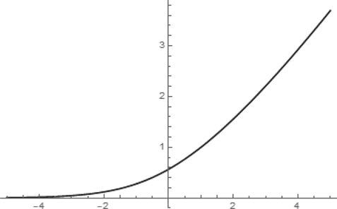
FIGURE 26 The plot of ω:ℝ→ ]0,∞[.

Moreover, ω is single-valued: for any fixed z∈ℂ, ω(z) is unique. This useful property of ω follows from the same property of exp, and K.

ω solves x+log⁡x=z

To see how to solve (3.17), we first take the exponential of both sides of (3.17):

ex+log⁡x=ez ex·x=ez,

and therefore x=Wk(ez) is a solution for some branch(es) of W. We shall show that the solution (if exists) is unique, except on a half-line. There is another half-line on which there is no solution at all.

Firstly, recall (3.15). Replace z with e^z in the second part of this formula:

Wk(ez)+log⁡Wk(ez)=log⁡(ez)+2πik.

We are well aware that log⁡(ez) is not z in general; instead, log⁡(ez)=z−2πiK(z) holds true (see (3.7)). Hence

Wk(ez)+log⁡Wk(ez)=z+2πi(k−K(z)),(3.19)

except when k=−1, and −1/e≤ez<0. Since x=Wk(ez) for some k, and x+log⁡x=y, it must hold true that Wk(ez)+log⁡Wk(ez)=z. According to (3.19), this is only possible in the non-exceptional case, when k=K(z). Thus, WK(z)(ez)=ω(z) is a solution. This finding tells why the definition of ω is given as it is.

In the exceptional case, we instead have that

Wk(ez)+log⁡Wk(ez)=z−2πiK(z),

so K(z)=0 must hold. This amounts to another solution if z is a complex number such that −1/e≤ez<0, and k=−1. Let us see, what are the possible values of z in this case. Let z=s+it; then ez=eseit. If we want this number to be negative and real, t=π+2lπ is necessary for some integer l. At the same time, K(z)=0 must hold, and this is only possible if l=0. Remark, that if l=−1, the number z still satisfies the inequality −1/e≤ez<0, but for this z we have K(z)=−1≠0. Thus, on the set

L0={t−iπ:−∞<t≤−1}

there is no solution of (3.17) at all.

Hence, t=π is the only possible case, and −1/e≤z=−es<0 holds only if s∈]−∞,−1]. We have got that W−1(ez) is a solution for any z for which ℜ(z)∈]−∞,−1] and ℑ(z)=π.

Notice, that for any such z, W0(ez) is another solution. Indeed, for such z, K(z)=0, and the non-exceptional case is applied. Thus, there are exactly two solutions of (3.17) if z belongs to the line

L2={t+iπ:−∞<t≤−1}.

Because of this fact, the line L₂ is called doubling line. For an illustration of L₀ and L₂, see Figure 27.

FIGURE 27 The lines L₀ and L₂.

The two solutions on L₂ are W0(ez) and W−1(ez). The first one is just W0(ez)=WK(z)(ez)=ω(z). We would like to express W−1(ez) in terms of ω, too. We have, on L, that W−1(ez)=W−1(ez−2πi)=WK(z−2πi)(ez−2πi)=ω(z−2πi).

Let us collect what we have deduced: the equation x+log⁡x=z has exactly one solution if z∈ℂ∖(L0∪L2), and this solution is x=ω(z). If z∈L0, the equation has no solution at all. Finally, if z∈L2, the equation has two solutions: x1=ω(z), and x2=ω(z−2πi).

Expressing W in terms of ω

The omega function is defined in terms of W, but this relation can be reversed: the Lambert W can be calculated from ω in a nice and simple way. This is advantageous because the ω function is single-valued, while W is multi-valued. So, a simple parameterization of ω gives the value of W on an arbitrary branch.

We will prove the following statement:

Wk(z)=ω(log⁡(z)+2πik) (z∈ℂ*, k∈ℤ).(3.20)

Here log⁡(z) is meant to be the principal branch of the logarithm.

In fact, our presentation for the solutions of (3.17) already demonstrates the validity of our statement. If z is a non-zero complex number not belonging to L₀ and L₂, it comes that, as we saw, ω(z)=Wk(ez), and thus

ω(log⁡z+2πik)=WK(log⁡z+2πik)(elog⁡z+2πik)=Wk(z).

In the last step, we used the fact that log refers to the principal branch, so −π<arg⁡(log⁡(z))≤π, hence K(log⁡(z)+2πik)=k.

3.4.3 The mapping properties of ω

There are some subtleties in the mapping properties of ω which are good to see in detail. The following facts are easy to see:

ω{ez:z∈ℂ, ℑ(z)∈]−3π,−π]}=W−1(ℂ*),ω{ez:z∈ℂ, ℑ(z)∈]−π,π]}=W0(ℂ*),ω{ez:z∈ℂ, ℑ(z)∈]π,3π]}=W1(ℂ*),etc.

This means that every horizontal strip of Figure 4 is mapped onto the corresponding area of Figure 13 (with the closures respected). In particular, ω maps ℂ onto ℂ^*. Zero is excluded, because W(z)=0 only when z=0, but the exponential in its argument never takes the value zero.

The images of L0 and L2 by ω

We shall show now, that there is a value, which is taken twice by omega. In order to see this, we check the image of L₀ and L₂ by ω. On all the points of L₂, the unwinding number is zero,; therefore

ω(L2)=W0(exp⁡(L2))=W0−1e,0=[−1,0[ ,

by (1.56). In particular,

ω(−1+iπ)=−1.

Next, we determine ω(L0). On L₀ the unwinding number is minus one everywhere, thus

ω(L0)=W−1(exp⁡(L0))=W−1−1e,0=]−∞,−1].

This is seen from (1.55). It follows that

ω(−1−iπ)=−1.

For a visual illustration of ω(L0) and ω(L2), see Figure 28.

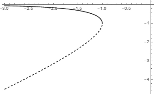
FIGURE 28 The plot of ω(L2) (continuous plot) and ω(L0) (dashed plot).

The existence of the doubling line causes that ω is not the straight functional inverse of z+log⁡z. Instead, the following result is valid:

ω−1(z)=z+ln⁡z−2πi−∞<z<−1−1±iπz=−1z+ln⁡z otherwise 

The proof of this fact is elementary, although a bit tedious because of the discontinuity of omega on the L₀ and L₂ lines. Regarding the continuity, we have the following result:

1. ω is analytic except at z=t±iπ for t≤−1.

2. For t≤−1, we have

   1. (a) ωt+iπ−=ω(t+iπ)=ωt−iπ−

   2. (b) ωt+iπ+=ω(t−iπ)=ωt−iπ+

We refer to [43] for the proofs. In the same paper, we can find the following table of special values of omega.

3.5 The branch difference function Mm,n

The difference between two branches of the logarithm at the same point is a multiple of 2π. Indeed, for a fixed z∈ℂ*

log⁡m(z)−log⁡n(z)=

log⁡|z|+i(arg⁡(z)+2mπi)−log⁡|z|−i(arg⁡(z)+2nπi)=2π(m−n).

This observation leads to the question about the branch difference of the Lambert W function². We define

Mm,n(z)=Wm(z)−Wn(z).

As the Lambert function satisfies the equation W(z)eW(z)=z, the function Mm,n(z) satisfies an equation, too. The elaboration of this statement will be given in the next subsection.

3.5.1 An equation for Mm,n(z)

Let z∈ℂ be a fixed number, and let x be a variable. Consider the equation

xe−x−1exp⁡xe−x−1=z.(3.21)

This equation has infinitely many solutions xm,n, and these are given as

xm,n=Mm,n(z) (m,n∈ℤ).

_______________________

²The branch difference function was defined in 2014 by D. J. Jeffrey and J. E. Jankowski [91].

Let us see why the branch difference function solves this equation. First, observe that

exp⁡Mm,n(z)=exp⁡Wm(z)exp⁡(Wn(z))

for all m,n∈ℤ. By (1.20) (which is valid for every branch) we eliminate the exponential on the right-hand-side:

exp⁡Mm,n(z)=Wn(z)Wm(z).(3.22)

From here, we can proceed in two ways. Either we substitute Mm,n(z)+Wn(z) in place of Wm(z), or we substitute Wm(z)−Mm,n(z) in place of Wn(z):

exp⁡Mm,n(z)=Wn(z)Mm,n(z)+Wn(z),exp⁡Mm,n(z)=Wm(z)−Mm,n(z)Wm(z).

Then these equations can be solved for Wn(z), and Wm(z), respectively:

Wn(z)=Mm,n(z)exp⁡−Mm,n(z)−1,

and

Wm(z)=Mm,n(z)1−exp⁡Mm,n(z).

Take the exponential of both sides of the individual equations, and use the fact that Wn(z)eWn(z)=z. We therefore get that if x=Mn,m(z), this x indeed solves (3.21).

We still have to show that if x is a solution, then x=Mm,n(z) for some m and n. Equation (3.21) is of the form ueu=z, so u=Wn(z) for some integer n. In other words,

u=xe−x−1=Wn(z).(3.23)

If we want to show that x=Wm(z)−Wn(z), it is better to fix x in the form

x=v−Wn(z),(3.24)

and try to show that v=Wm(z). Multiply both sides of the last displayed equation by minus one, and take the exponential:

e−x=eWn(z)e−v=zWn(z)e−v.

Substitute this and (3.24) into (3.23). It turns out that the resulting equation is solvable in terms of the W function:

v=Wm(z), for some m.

This is what we wanted to prove.

3.5.2 An equation for M0,−1(z)

There is another special equation which can be solved by the branch difference function, but now we only need the parameters m=0, n=−1.

The equation

xe−xcoth⁡xcschx=z(3.25)

has a real solution for 0<z≤1/e:

x=±12M0,−1(−z).(3.26)

In the equation coth is the hyperbolic cotangent:

coth⁡x=ex+e−xex−e−x=e2x+1e2x−1,

and csch is the hyperbolic cosecant:

cschx=1sinh⁡x=2ex−e−x.

The proof is as follows. An inspection of Figure 29 shows that the function on the left-hand side of (3.25) is even in x, thus it suffices to consider only the set x≥0. Moreover, the function takes values from the interval ]0,−1/e]; therefore, we see that the restriction on z is necessary. The maximum is taken for x=0, where the value of the left-hand side is 1/e.

FIGURE 29 The plot of xe−xcoth⁡xcschx on the interval [−5,5].

If z is from the interval ]0,1/e], the range of M0,−1(−z)=W0(−z)−W−1(z) is [0,∞[ (this follows from (1.55)-(1.56)). This is in agreement with our restriction that x≥0.

Since the left-hand side is strictly decreasing over the positive axis, it is enough to show that 12M0,−1(−z) is indeed a solution (over the positive reals). Substituting (3.26) into xcschx, we get that

xcschx=M0,−1(−z)exp⁡(M0,−1(−z)/2)−exp⁡(−M0,−1(−z/2)).

By (3.22), the right-hand-side is rewritten as

M0,−1(−z)exp⁡(M0,−1(−z)/2)−exp⁡(−M0,−1(−z/2))=−W0(−z)W−1(−z)W0(−z)=

=−W0(−z)W−1(−z)W0(−z)W02(−z)=W−1(−z)W0(−z).

(Care needs to be taken when manipulating the square roots.) We thus get that

xcschx=W−1(−z)W0(−z).

With the same approach, substituting (3.26) into e−xcoth⁡x:

e−xcoth⁡x=z2W0(−z)W−1(−z).

Multiplying what we have got for xcschx and for e−xcoth⁡x, the statement follows.

Finally, we remark that, upon substituting x=iy, and recalling the identities

coth⁡(ix)=−icot⁡x,csch(ix)=−icsc⁡x=−isin⁡z,

equation (3.25) can be put in another form:

ysin⁡ye−ycot⁡y=z,(3.27)

and the solution is then

y=±i2M0,−1(−z).

The range of M0,−1(z)

In [91] the range of the function

M0,−1:ℂ→ℂ

was determined. This function maps ℂ onto the region of ℂ surrounded by the positive real and imaginary axes, and by the two curves

C1={W0(x)−W−2(x):x∈[−1/e,0[},C2={W−1(x)−W−2(x):x∈]−∞,−1/e[}.

See Figure 30 where this region is depicted.

FIGURE 30 The range of the branch difference function M0,−1. The vertical line segment goes up to 2πi. The wall is the curve C₂ and the upmost curve reaching out to plus infinity is C₁.

Further notes

1. Computer algebra. We saw in this chapter that it is often suggested to unlearn our high-school routine when doing calculations with complex numbers, because usual identities might fail. At the dawn of computer programming, even professional programmers wrote erroneous codes. N. Higham [81] notes that it took five papers and three years to get the complex logarithm in the Algol 60 language right. H. Aslaksen [10] gave tests for users of mathematical software to check the capabilities of their systems. The introduction of the unwinding number and agreement on branch cuts of the usual inverse functions (sin⁡−1, sinh⁡−1, etc.) highly uniformized and simplified the programming; see [49, 99] for some historical insight, and [25, 40, 87, 88, 99, 146] for practical suggestions for computer algebra systems.

   About the implementation of the Lambert function in Maple, see [89].

2. A physical application of equation (3.27). Although (3.27) seems to be rather artificial, it does have applications: it occurs in the study of dispersion equations for damped plasma oscillations. See [5] for details, especially around equation (15) there.