
Introduction to Equity Valuation and Investing
Intrinsic value is an all-important concept that offers the only logical approach to evaluating the relative attractiveness of investments and businesses. Intrinsic value can be defined simply: It is the discounted value of the cash that can be taken out of a business during its remaining life.
—Warren Buffett
This part of the book describes equity strategies, also called stock selection strategies. Stock selection strategies seek to determine which stocks have high expected returns and which have low expected returns. Hedge funds then seek to buy the high-expected-return stocks and short the low-expected-return ones. Similarly, active long-only equity investors seek to overweight the high-expected-return stocks and underweight, or altogether avoid, the low-expected-return ones.
I consider three types of equity strategies: discretionary equity investments (chapter 7), dedicated short bias (chapter 8), and quantitative equity (chapter 9). Discretionary equity investment is the classic, and most common, form of equity trading, pursued by long–short equity hedge funds, active equity mutual funds, and others. Discretionary equity investment means that the traders and portfolio managers buy stocks based on their discretionary views, that is, their overall assessment of the stocks that they have analyzed. Discretionary traders perform a tailored analysis of each stock under consideration based on all kinds of information, including equity valuation models, discussions with the firms’ management, competitors, intuition, and experience. Typically discretionary equity investors buy more stocks than they sell short, but the reverse is true for dedicated short bias hedge funds. Dedicated short bias hedge funds focus on findings stocks that are about to go down, looking for frauds, overstated earnings, or poor business plans. Dedicated short bias hedge funds rely on a fundamental analysis of companies in a similar way to other discretionary equity investors.
Discretionary trading can be seen in contrast to quantitative trading, which invests systematically based on a model. Both types of traders may seek lots of data and use valuation models, but whereas discretionary traders make their final trading decisions based on human judgment, quantitative investors trade systematically with minimal human interference. Quantitative investors gather data, check the data, feed it into a model, and let the model send trades to the exchanges.1
Quants try to develop a small edge on each of many small diversified trades using sophisticated processing of ideas that cannot be easily processed using non-quantitative methods. To do this, they use tools and insights from economics, finance, statistics, math, computer science, and engineering, combined with lots of data (public and proprietary) to identify relationships that market participants may not have incorporated in the price immediately. They build computer systems that generate trading signals based on these relations, perform portfolio optimization in light of trading costs, and trade using automated execution schemes that route hundreds of orders every few seconds. In other words, trading is done by feeding data into computers that run various programs with human oversight.
Discretionary trading has the advantages of a tailored analysis of each trade and the use of a lot of soft information such as private conversations, but its labor-intensive method implies that only a limited number of securities can be analyzed in depth, and the discretion exposes the trader to psychological biases. Quantitative trading has the advantage of discipline, an ability to apply a trading idea to a wide universe of securities with the benefits of diversification, and efficient portfolio construction, but it must rely only on hard data and the computer program’s limited ability to incorporate real-time judgment.
While the three forms of equity investment have several differences, each relies on an understanding of equity valuation. As the quote above by Warren Buffett makes clear, a stock’s intrinsic value is at the heart of equity valuation, as we discuss in this chapter.
6.1. EFFICIENTLY INEFFICIENT EQUITY MARKETS
Before we go into the details of deriving a stock’s intrinsic value, let us recall what it is used for, namely value investing. Value investors seek to buy cheap stocks, i.e., those with a low market value relative to the intrinsic value. Similarly, value investors short-sell expensive stocks with higher market valuations than intrinsic value.
Value investors make the market more efficient. They bring prices closer to fundamentals as they push up the prices of cheap stocks and push down the prices of expensive stocks. However, competition among value investors does not fully eliminate all inefficiencies since value investing involves fundamental risk and liquidity risk. If you buy a cheap stock for a price below the expected future profits, you can still lose money if unforeseen events harm the firm or if you are forced to sell before the stock price rises. Hence, investors need a premium for incurring these risks, leaving stocks with an efficient level of inefficiency. Said differently, the market has an efficient spread between prices and fundamentals that value investors, sometimes call their margin of safety (as discussed further below). The efficiently inefficient equity market has the property that prices can wander further from their fundamental values for illiquid stocks that are expensive to trade, volatile stocks that are risky to trade, stocks with large supply/demand imbalances, and stocks that are costly to short-sell, especially when active investors are facing reductions in capital and financing opportunities.
6.2. INTRINSIC VALUE AND THE DIVIDEND DISCOUNT MODEL
The foundation for trading equities is understanding equity valuation. The value of a stock is often called its intrinsic value (or fundamental value) to distinguish it from the market price. Whereas believers in market efficiency consider the price and the intrinsic value to be the same, believers in value investing look for stocks where the market price is cheap relative to the intrinsic value. Indeed, intrinsic value is at the very heart of value investing, as seen from the Warren Buffett quote above.
Let us consider a stock’s intrinsic value Vt at a certain time t. The intrinsic value ultimately derives from the free cash that can be returned to shareholders. We will refer to these free cash flows as the “dividends” Dt, but they should be interpreted broadly as all cash returned to shareholders (including capital returned through share repurchases), less the capital that needs to be injected by shareholders (through seasoned equity offerings).
Of course, we cannot just add up dividends across different time periods because we must account for the time value of money and the uncertainty of the future cash flows. We start by considering how the value today depends on what happens over the next time period, say the next year. Today’s intrinsic value depends on the next dividend Dt+1, the value next period, and the required rate of return kt (also called the discount rate) over this time period. Specifically, the current value is the expected discounted value of the dividend and value next period:
Hence, to value a stock, we must be able to estimate the expected dividend payment next time period. We also need to decide on the required rate of return kt, which naturally depends on the riskiness of the stock. For instance, an equity trader might estimate a stock’s market beta as β = 1.2, the market risk premium as E(RM − Rf) = 5%, and the current risk-free rate as Rf = 2%. The trader might then use the capital asset pricing model (CAPM) to conclude that the stock’s required return is kt = 2% + 1.2 ∙ 5% = 8%.
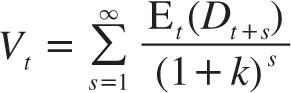
Lastly, to determine the intrinsic value at the current time t, it might seem that we need to estimate the intrinsic value next time period, t + 1. However, rather than doing that, we use the valuation equation repeatedly to arrive at

This equation shows mathematically what the Buffett quote above says in words, namely that the intrinsic value is the expected discounted value of all future dividends paid to shareholders. This equation is called the dividend discount model (and it is also called the discounted cash flow model and the present value model).
Computing the intrinsic value is easier said than done, easier in principle than in practice.2 To compute the intrinsic value, one must estimate all future dividends, all future discount rates, and the co-movement of future dividends and discount rates. To simplify this task, equity traders often assume a constant discount rate so that kt = k for all t. In this case, the valuation formula simplifies as follows:
Gordon’s Growth Model
The dividend discount model can be further simplified by assuming a constant expected dividend growth. A constant dividend growth means that Et (Dt+s) = (1 + g)sDt, where g is the growth rate. With this assumption, the intrinsic value reduces to an intuitive expression:
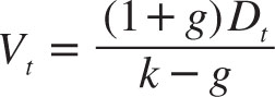
The intrinsic value is naturally higher if current dividends are higher, if the dividend growth rate is higher, or if the required return is lower.
Multi-Stage Dividend Discount Models
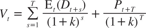
Gordon’s growth model is only appropriate for firms with a constant growth rate and, furthermore, it requires that the growth rate g be less than the discount rate k (otherwise, the denominator in Gordon’s growth model would be negative, reflecting that such a high growth rate relative to the discount rate cannot be achieved in a long-run equilibrium). However, equity investors often become interested in firms that are going through unusual events, and such firms might experience several years of unusually high growth, including periods with g > k. Similarly, firms can experience periods of temporary contraction. In such cases, the current value of the stock can be computed as the present value of the dividends during the unusual time period plus the terminal value:
Here, the terminal value Pt+T can be estimated by assuming a constant growth rate at that future time and using Gordon’s growth model. Alternatively, Pt+T can be computed by assuming an industry-typical valuation ratio at that time, e.g., as 40 times Et(Dt+T) if firms in this industry tend to trade at a price-dividend ratio of 40-to-1 (see the section on “relative valuation” below). The dividends between time t and time t + T can be estimated by separately estimating all the cash flows during these years—value investors are known for spreadsheets full of such numbers. Alternatively, you can assume that the stock will experience an unusual, but constant, growth of g for the first T years. Then current value of such a stock is
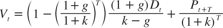
This equation is called the two-stage dividend discount model because the growth is assumed to have a constant rate in an initial “stage” (from time t to time t + T) and at another constant rate in the second stage (the time after t + T), which is used to compute the terminal value. (Note that this expression is positive even when the initial growth is above the discount rate, g > k.)
To summarize, the general idea is that valuation is based on the dividend discount model, and we can get some simple expressions by assuming a constant growth over certain time periods (based on the well-known formula for the sum of geometric series). Some equity investors take this idea further and consider three-stage and other more complex multi-stage valuation models.
6.3. EARNINGS, BOOK VALUES, AND THE RESIDUAL INCOME MODEL
For some firms, estimating dividends is difficult, for instance, because young firms tend to retain earnings for a number of years until they finally mature and start paying out dividends. More broadly, it is sometimes more natural to focus on a firm’s economic earnings than its dividend payments. The two concepts are closely linked: to pay out dividends, the firm must earn profits, and earnings must ultimately be returned to shareholders to have consumption value.
To formally link earnings and dividends, we define the earnings as the net income, NIt, and also keep track of the stock’s book value, Bt. The book value is increased by the net income and reduced by capital paid out as dividends, and this key link is called the “clean surplus accounting relation”:
![]()
If we solve for dividends in the clean surplus relation and plug this expression into the dividend discount model, then we get the residual income model:3
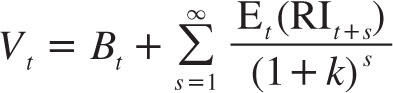
where the residual income, RI, is defined as
![]()
The residual income model says that the intrinsic value of the stock is equal to the book value plus the present value of the entire stream of future residual income. What is residual income? It is the amount of earnings NIt over and above the cost of book equity, where the cost of book equity is the required return k times the level of book equity in the previous time period Bt–1. Naturally, residual income on any date t can be positive or negative. Residual income is of course negative if the earning is negative, but residual income can also be negative with a positive earning that is smaller than the cost of capital. If the present value of all residual incomes is negative, this result corresponds to the intrinsic value being below the book value; otherwise, the intrinsic value is above the book value.
In summary, the intrinsic value is the current book value plus the present value of the additional (or residual) future profits that we expect to earn—above what could be expected based on the current book equity.
6.4. OTHER APPROACHES TO EQUITY VALUATION
Relative Valuation
Equity investors often value stocks based on the valuation of other comparable stocks. For instance, they might value a stock at E × P/E, where E is the firm’s earnings and P/E is the price-to-earnings ratio of comparable stocks, e.g., the average within the industry. This same method can in principle be used for any number of valuation ratios, but the important thing is that the firm’s current characteristic (e.g., the current earnings E) is representative of the firm and its future prospects (not a one-year fluke number) and that the valuation ratio comes from a comparable set of stocks. Of course, relative valuation cannot tell you whether the entire stock market is over- or undervalued, but it can be informative about which stocks are expensive or cheap relative to others.
Implied Expected Returns
Another approach is to use the current price and the estimated future cash flows to compute each stock’s “implied expected return” in the sense of its internal rate of return, also called the implied cost of capital. Based on such estimates of each stock’s implied expected returns, a value investor might go long on those with high expected returns and short those with low ones.4
Firm Value vs. Equity Value
The same principles can naturally be used to value an entire firm (also called enterprise valuation) and its equity. Of course, the equity is worth less than the enterprise if the enterprise has debt. To value the enterprise or the equity, the key is to make sure that all inputs are “apples-to-apples.” In particular, when valuing equity, one must consider the required return of the equity (which is riskier than the enterprise due to the leverage effect) and the free cash flows to equity holders (i.e., dividends). When valuing the enterprise, one must compute the present value of the free cash flows to the whole firm, that is, earnings before debt payments (but after all other cash drains, including reinvestment needs).
Similarly, when computing financial ratios, one should make sure that the numerator and denominator are apples-to-apples: If the numerator is an equity-level variable (as opposed to enterprise-level), then so should the denominator be. For instance, we consider a stock’s price-to-earnings ratio, not its enterprise value-to-earnings ratio because the latter would look bad for a leveraged firm just because the interest payments reduce the earnings. Hence, with enterprise value in the numerator, the denominator should have earnings before interest expenses.
___________________
1 Quantitative traders are close cousins to, but perform different roles than, the “sell-side quants” described in Emanuel Derman’s interesting autobiography My Life as a Quant (2004). Sell-side quants provide analytical tools that are helpful for hedging, risk management, discretionary traders, clients, and other purposes. In contrast, quantitative traders work on the “buy-side” and build models that are used directly as a tool for systematic trading.
2 See Damodaran (2012) for an extensive description of equity valuation and financial statement analysis.
3 To see this result, first note that
![]()
Then change index on the first book value and make the appropriate adjustments to arrive at
![]()
which gives the residual income model. This version of the dividend discount model goes back to Preinreich (1938).
4 See Hou, van Dijk, and Zhang (2012) and references therein.