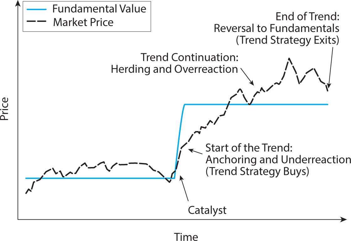
Figure 12.1. Stylized plot of the life cycle of a trend.
Source: Hurst, Ooi, and Pedersen (2013).
Managed Futures
Trend-Following Investing
Cut short your losses … and let your profits run on.
—David Ricardo (1772–1823)
… big money was not in the individual fluctuations but in … sizing up the entire market and its trend.
—Jesse Livermore
David Ricardo’s imperative, which has survived two centuries, suggests an attention to trends.1 Trends are also at the heart of the century-old statement by the legendary trader Jesse Livermore, and trends continue to play an important role for active investors. The traders who are most directly focused on trend-following investing are the managed futures hedge funds and commodity trading advisors (CTAs). Such funds have existed at least since Richard Donchian started his fund in 1949, and they have proliferated since the 1970s when futures exchanges expanded the set of tradable contracts. BarclayHedge estimates that the CTA industry has grown, managing approximately $320 billion as of the end of the first quarter of 2012.2
Managed futures returns can be largely understood by simple, implementable trend-following strategies—specifically time series momentum strategies. This chapter provides a detailed analysis of the economics of these strategies and applies them to explain the properties of managed futures funds. Using the returns to time series momentum strategies, we analyze how managed futures funds benefit from trends and how they rely on different trend horizons and asset classes, and we examine the role of transaction costs and fees within these strategies.
Time series momentum is a simple trend-following strategy that goes long on a market that has experienced a positive excess return over a certain look-back horizon and goes short otherwise. We consider 1-month, 3-month, and 12-month look-back horizons (corresponding to short-term, medium-term, and long-term trend strategies) and implement the strategies for a liquid set of commodity futures, equity futures, currency forwards, and government bond futures.
Trend-following strategies only produce positive returns if market prices exhibit trends, but why should price trends exist? We discuss the economics of trends based on initial underreaction to news and delayed overreaction as well as the extensive literature on behavioral biases, herding, central bank behavior, and capital market frictions. If prices initially underreact to news, then trends arise as prices slowly move to more fully reflect changes in fundamental value. These trends have the potential to continue even further due to a delayed overreaction from herding investors. Naturally, all trends must eventually come to an end as deviation from fair value cannot continue indefinitely.
We find strong evidence of trends across different look-back horizons and asset classes. A time series momentum strategy that is diversified across all assets and trend horizons realizes a gross Sharpe ratio of 1.8 with little correlation to traditional asset classes. In fact, the strategy has produced its best performance in extreme up and extreme down stock markets. One reason for the strong performance in extreme markets is that most extreme bear or bull markets historically have not happened overnight but have occurred over several months or years. Hence, in prolonged bear markets, time series momentum takes short positions as markets begin to decline and thus profits as markets continue to fall.
Time series momentum strategies help explain returns to the managed futures universe. Like time series momentum, some managed futures funds have realized low correlation to traditional asset classes, performed best in extreme up and down stocks markets, and delivered alpha relative to traditional asset classes.
When we regress managed futures indices and manager returns on time series momentum returns, we find large R-squares and very significant loadings on time series momentum at each trend horizon and in each asset class. In addition to explaining the time variation of managed futures returns, time series momentum also explains the average excess return. Indeed, controlling for time series momentum drives the alphas of most managers and indices below zero. The negative alphas relative to the hypothetical time series momentum strategies show the importance of fees and transaction costs. Comparing the relative loadings, we see that most managers focus on medium- and long-term trends, giving less weight to short-term trends, and some managers appear to focus on fixed-income markets.
12.1. THE LIFE CYCLE OF A TREND
The economic rationale underlying trend-following strategies is illustrated in figure 12.1, a stylized “life cycle” of a trend. An initial underreaction to a shift in fundamental value allows a trend-following strategy to invest before new information is fully reflected in prices. The trend then extends beyond fundamentals due to herding effects and finally results in a reversal. We discuss the drivers of each phase of this stylized trend, as well as the related literature.
Start of the Trend: Underreaction to Information
In the stylized example shown in figure 12.1, a catalyst—a positive earnings release, a supply shock, or a demand shift—causes the value of an equity, commodity, currency, or bond to change. The change in value is immediate, shown by the solid line. While the market price (shown by the dashed line) moves up as a result of the catalyst, it initially underreacts and therefore continues to go up for a while. A trend-following strategy buys the asset as a result of the initial upward price move and therefore capitalizes on the subsequent price increases. At this point in the life cycle, trend-following investors contribute to the speeding up of the price discovery process.
Figure 12.1. Stylized plot of the life cycle of a trend.
Source: Hurst, Ooi, and Pedersen (2013).
Research has documented a number of behavioral tendencies and market frictions that lead to this initial underreaction:3
i. Anchor-and-insufficient-adjustment. People tend to anchor their views to historical data and adjust their views insufficiently to new information.
ii. The disposition effect. People tend to sell winners too early and ride losers too long. They sell winners early because they like to realize their gains. This creates downward price pressure, which slows the upward price adjustment to new positive information. On the other hand, people hang on to losers because realizing losses is painful. They try to “make back” what has been lost. Fewer willing sellers can keep prices from adjusting downward as fast as they should.
iii. Non-profit-seeking activities. Central banks operate in the currency and fixed-income markets to reduce exchange-rate and interest-rate volatility, potentially slowing the price adjustment to news. Also, investors who mechanically rebalance to strategic asset allocation weights trade against trends. For example, a 60/40 investor who seeks to own 60% stocks and 40% bonds will sell stocks (and buy bonds) whenever stocks have outperformed.
iv. Frictions and slow moving capital. Frictions, delayed response by some market participants, and slow-moving arbitrage capital can also slow price discovery and lead to a drop and rebound of prices.
The combined effect is for the price to move too gradually in response to news, creating a price drift as the market price slowly incorporates the full effect of the news. A trend-following strategy will position itself in relation to the initial news and profit if the trend continues.
Trend Continuation: Delayed Overreaction
Once a trend has started, a number of other phenomena exist which may extend the trend beyond the fundamental value:4
i. Herding and feedback trading. When prices have moved in one direction for a while, some traders may jump on the bandwagon because of herding or feedback trading. Herding has been documented among equity analysts in their recommendations and earnings forecasts, in investment newsletters, and in institutional investment decisions.
ii. Confirmation bias and representativeness. These heuristics show that people tend to look for information that confirms what they already believe and to look at recent price moves as representative of the future. This attitude can lead investors to move capital into investments that have recently made money and conversely out of investments that have declined, both of which cause trends to continue.
iii. Fund flows and risk management. Fund flows often chase recent performance (perhaps because of i. and ii.). As investors pull money from underperforming managers, these managers respond by reducing their positions (which have been underperforming), while outperforming managers receive inflows, adding buying pressure to their outperforming positions. Furthermore, some risk-management schemes imply selling in down markets and buying in up markets, in line with the trend. Examples of this behavior include stop-loss orders, portfolio insurance, and corporate hedging activity (e.g., an airline company that buys oil futures after the oil price has risen to protect the profit margins from falling too much, or a multinational company that hedges foreign exchange exposure after a currency moved against it).
End of the Trend
Obviously, trends cannot go on forever. At some point, prices extend too far beyond fundamental value and, as people recognize this, prices revert toward the fundamental value and the trend dies out. As evidence of such overextended trends, extended price moves that have occurred over 3–5 years tend to partly be reversed.5 The return reversal only reverses part of the initial price trend, suggesting that the price trend was partly driven by initial underreaction (since this part of the trend should not reverse) and partly driven by delayed overreaction (since this part reverses).
12.2. TRADING ON TRENDS
Having discussed why trends might exist, we now demonstrate the performance of a simple trend-following strategy: time series momentum. We construct time series momentum strategies for 58 highly liquid futures and currency forwards from January 1985 to June 2012—specifically 24 commodity futures, 9 equity index futures, 13 bond futures, and 12 currency forwards. To determine the direction of the trend in each asset, the strategy simply considers whether the asset’s excess return is positive or negative: A positive past return is considered an “up trend” and leads to a long position; a negative return is considered a “down trend” and leads to a short position.
We consider 1-month, 3-month, and 12-month time series momentum strategies, corresponding to short-, medium-, and long-term trend-following strategies. The 1-month strategy goes long if the preceding 1-month excess return was positive and goes short if it was negative. The 3-month and 12-month strategies are constructed analogously. Hence, each strategy always holds a long or a short position in each of 58 markets.
The size of each position is chosen to target an annualized volatility of 40% for that asset.6 Specifically, the number of dollars bought/sold of instrument s at time t is 40%/ so that the time series momentum (TSMOM) strategy realizes the following return during the next week:

Here, is the ex ante annualized volatility for each instrument, estimated as an exponentially weighted average of past squared returns. This constant-volatility position-sizing methodology is useful for several reasons: First, it enables us to aggregate the different assets into a diversified portfolio that is not overly dependent on the riskier assets—this is important given the large dispersion in volatility among the assets we trade. Second, this methodology keeps the risk of each asset stable over time, so that the strategy’s performance is not overly dependent on what happens during times of high risk. Third, the methodology minimizes the risk of data mining given that it does not use any free parameters or optimization in choosing the position sizes.
The portfolio is rebalanced weekly at the closing price each Friday, based on data known at the end of each Thursday. We therefore are only using information available at the time to make the strategies implementable. The strategy returns are gross of transaction costs, but we note that the instruments we consider are among the most liquid in the world. Below we consider the effect of transaction costs and the use of different rebalance rules. Academics often consider monthly rebalancing, but it is interesting to also consider higher rebalancing frequencies, given our focus on explaining the returns of professional money managers who often trade throughout the day.
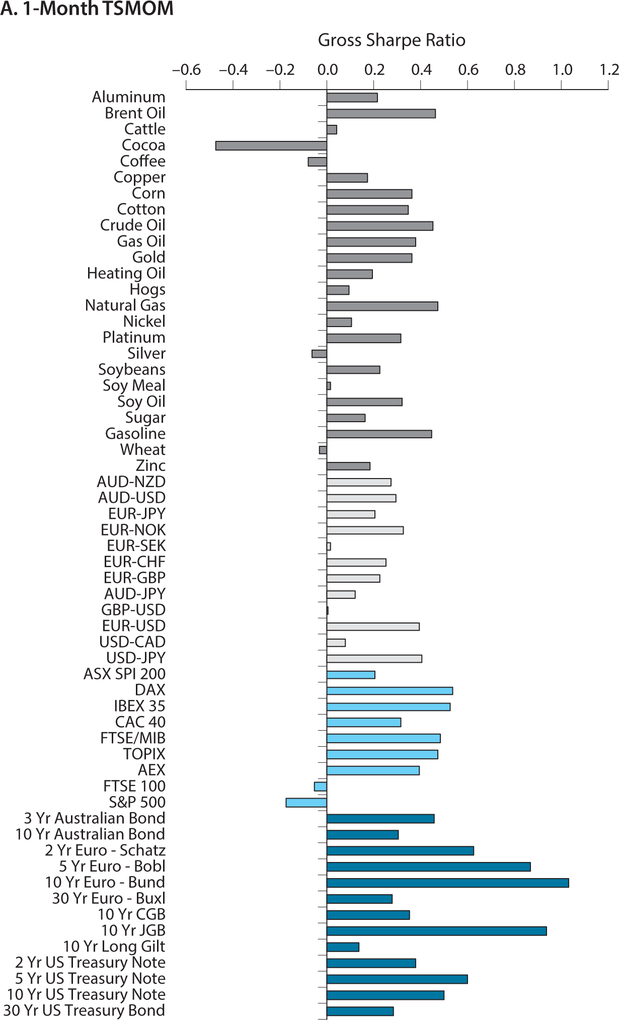
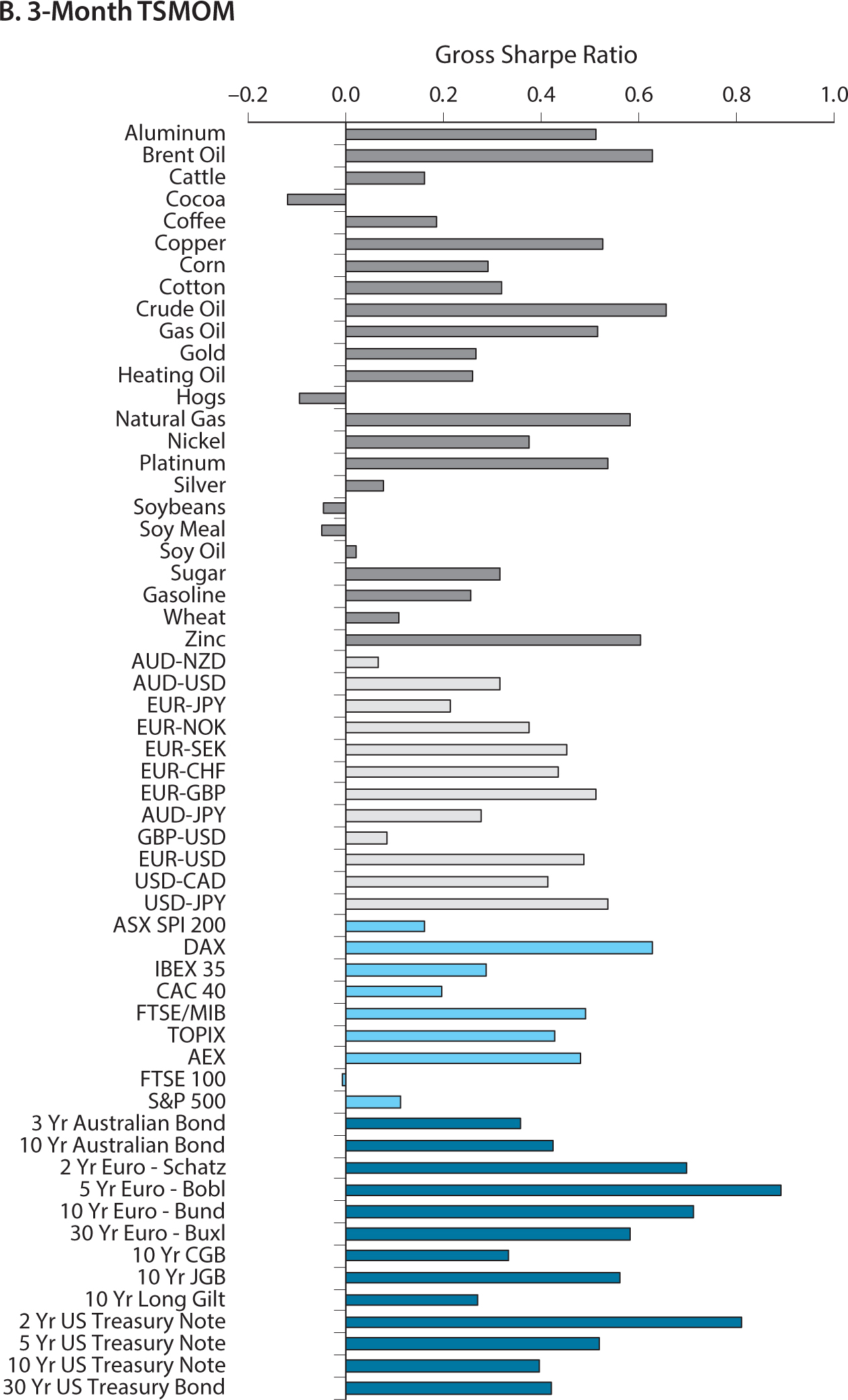
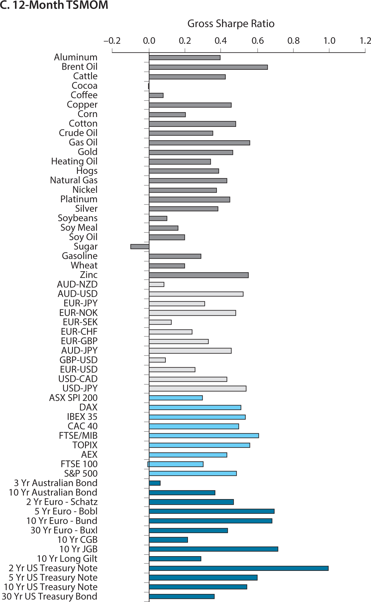
Figure 12.2 shows the performance of each time series momentum strategy in each instrument. The strategies deliver positive results in almost every case, a remarkably consistent result. The average Sharpe ratio (excess returns divided by realized volatility) across assets is 0.29 for the 1-month strategy, 0.36 for the 3-month strategy, and 0.38 for the 12-month strategy.
12.3. DIVERSIFIED TIME SERIES MOMENTUM STRATEGIES
Next, we construct diversified 1-month, 3-month, and 12-month time series momentum strategies by averaging returns of all the individual strategies that share the same look-back horizon (denoted TSMOM1M, TSMOM3M, and TSMOM12M, respectively). We also construct time series momentum strategies for each of the four asset classes: commodities, foreign exchange, equities, and fixed income (denoted TSMOMCOM, TSMOMFX, TSMOMEQ, and TSMOMFI, respectively). For example, the commodity strategy is the average return of each individual commodity strategy for all three trend horizons. Finally, we construct a strategy that diversifies across all assets and all trend horizons that we call the diversified time series momentum strategy (denoted simply TSMOM). In each case, we scale the positions to target an ex ante volatility of 10% using an exponentially weighted variance–covariance matrix.
Table 12.1 shows the performance of these diversified time series momentum strategies. We see that the strategies’ realized volatilities closely match the 10% ex ante target, varying from 9.5% to 11.9%. More importantly, all the time series momentum strategies have impressive Sharpe ratios, reflecting a high average excess return above the risk-free rate relative to the risk. Comparing the strategies across trend horizons, we see that the long-term (12-month) strategy has performed the best, the medium-term strategy has done second best, and the short-term strategy, which has the lowest Sharpe ratio of the three strategies, still has a high Sharpe ratio of 1.3. Comparing asset classes, commodities, fixed income, and currencies have performed a little better than equities.
Figure 12.2. Performance of time series momentum by individual asset and trend horizon.
This figure shows the Sharpe ratios of the time series momentum strategies for each commodity futures (dark grey), currency forward (light grey), equity futures (light blue), and fixed-income futures (dark blue). We show this for strategies using look-back horizons of 1 month (A), 3 months (B), and 12 months (C).
Source: Hurst, Ooi, and Pedersen (2013).
TABLE 12.1. PERFORMANCE OF TIME SERIES MOMENTUM (TSMOM) STRATEGIES
Panel A. Performance of TS-Momentum across Asset Classes
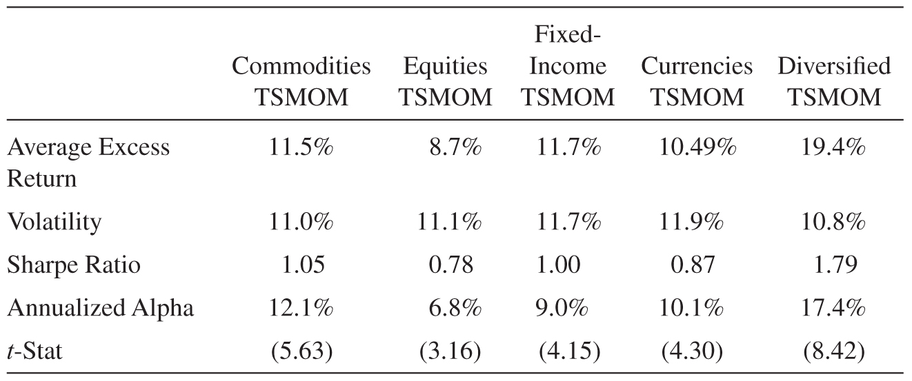
Panel B. Performance of Time Series Momentum across Signals
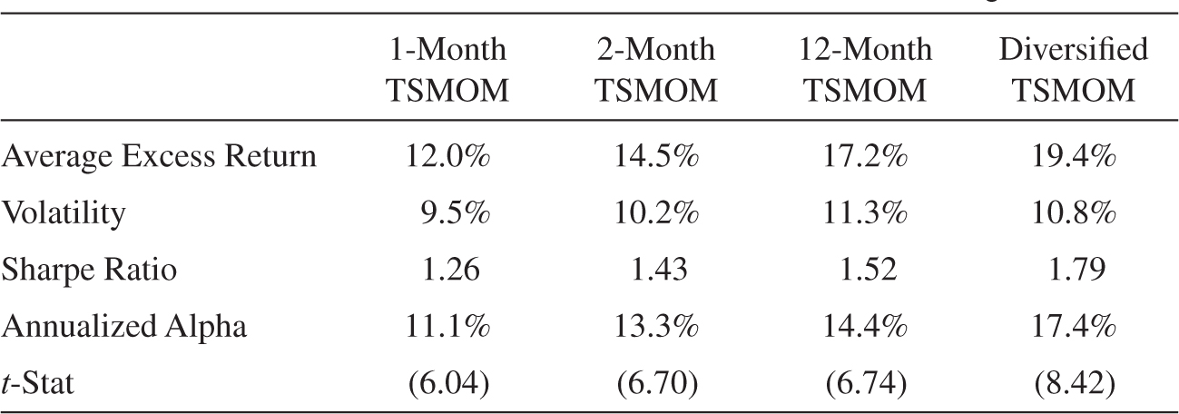
Notes: This table shows the performance of time series momentum strategies diversified within each asset class (Panel A) and across each trend horizon (Panel B). All numbers are annualized. The alpha is the intercept from a regression on the MCSI World stock index, Barclays Bond Index, and the GSCI commodities index. The t-statistic of the alpha is shown in parentheses.
Source: Hurst, Ooi, and Pedersen (2013).
In addition to reporting the expected return, volatility, and Sharpe ratio, table 12.1 also shows the alpha from the following regression:
![]()
We regress the TSMOM strategies on the returns of a passive investment in the MSCI World stock market index, the Barclays U.S. aggregate government bond index, and the S&P GSCI commodity index. The alpha measures the excess return, controlling for the risk premiums associated with simply being long in these traditional asset classes. The alphas are almost as large as the excess returns since the TSMOM strategies are long–short and therefore have small average loadings on these passive factors. Finally, table 12.1 reports the t-statistics of the alphas, which show that the alphas are highly statistically significant.
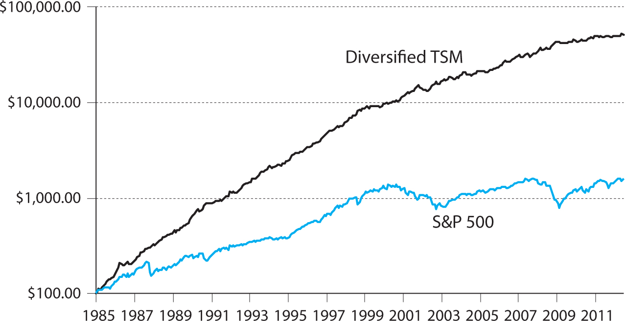
Figure 12.3. Performance of the diversified time series momentum strategy and the S&P 500 index over time.
The figure shows the cumulative return gross of transaction costs of the diversified TSMOM strategy and the S&P 500 equity index on a log scale, 1985–2012.
Source: Hurst, Ooi, and Pedersen (2013).
The best performing strategy is the diversified time series momentum strategy, with a Sharpe ratio of 1.8. Its consistent cumulative return is seen in figure 12.3, which illustrates the hypothetical growth of $100 invested in 1985 in the diversified TSMOM strategy and the S&P 500 stock market index, respectively.
12.4. DIVERSIFICATION: TRENDS WITH BENEFITS
To understand this strong performance of time series momentum, note first that the average pairwise correlation of these single-asset strategies is less than 0.1 for each trend horizon, meaning that the strategies behave rather independently across markets so one may profit when another loses. Even when the strategies are grouped by asset class or trend horizon, these relatively diversified strategies also have modest correlations. Another reason for the strong benefits of diversification is our equal-risk approach. The fact that we scale our positions so that each asset has the same ex ante volatility at each time means that, the higher the volatility of an asset, the smaller a position it has in the portfolio, creating a stable and risk-balanced portfolio. This is important because of the wide range of volatilities exhibited across assets. For example, a five-year U.S. government bond futures typically exhibits a volatility of around 5% a year, while a natural gas futures typically exhibits a volatility of around 50% a year. If a portfolio holds the same notional exposure to each asset in the portfolio (as some indices and managers do), the risk and returns of the portfolio will be dominated by the most volatile assets, significantly reducing the diversification benefits.
The diversified time series momentum strategy has very low average correlations to traditional asset classes. Indeed, the correlation with the S&P 500 stock market index is –0.02, the correlation with the bond market as represented by the Barclays U.S. aggregate index is 0.23, and the correlation with the S&P GSCI commodity index is 0.05. This low average correlation hides the fact that the strategy can at times be highly correlated to the market, but these correlations are offset on average by other times when the strategy is negatively correlated to the market.
Trend-following investing has performed especially well during periods of prolonged bear markets and in sustained bull markets, as seen in figure 12.4. Figure 12.4 plots the quarterly returns of time series momentum against the quarterly returns of the S&P 500. We estimate a quadratic function to fit the relation between time series momentum returns and market returns, giving rise to a “smile” curve. The estimated smile curve means that time series momentum has historically done the best during significant bear markets or significant bull markets, performing less well in flat markets. To understand this smile effect, note that most of the worst equity bear markets have historically happened gradually. The market first goes from “normal” to “bad,” causing a TSMOM strategy to go short (while incurring a loss or profit depending on what happened previously). Often, a deep bear market happens when the market goes from “bad” to “worse,” traders panic, and prices collapse. This leads to profits on the short positions, explaining why these strategies tend to be profitable during such extreme events. Of course, these strategies do not always profit during extreme events. For instance, the strategy might incur losses if, after a bull market (which would get the strategy positioned long), the market crashed quickly before the strategy could alter its positions to benefit from the crash.
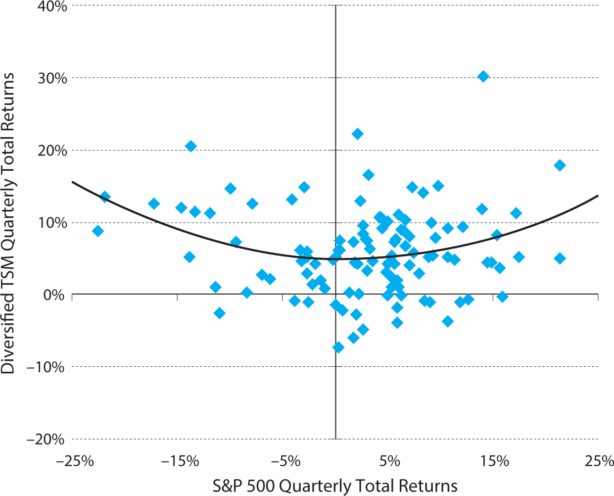
Figure 12.4. Time series momentum “smile.”
This graph plots quarterly non-overlapping hypothetical returns of the diversified time series momentum strategy vs. the S&P 500, 1985–2012.
Source: Hurst, Ooi, and Pedersen (2013).
12.5. TIME SERIES MOMENTUM EXPLAINS ACTUAL MANAGED FUTURES FUND RETURNS
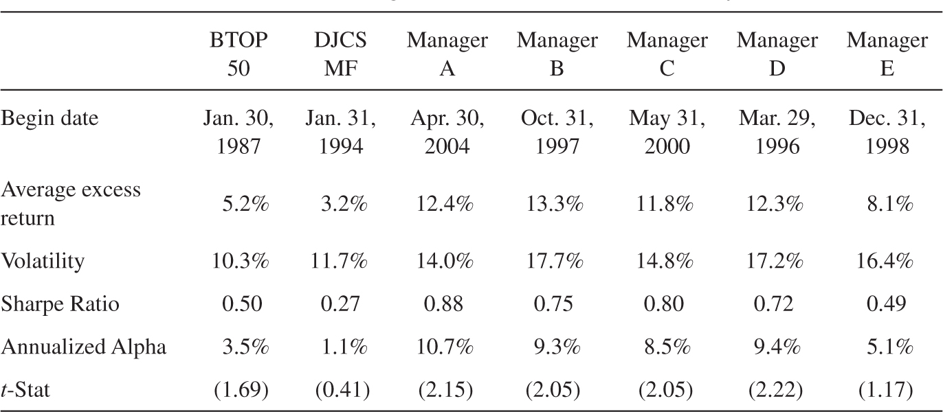
We collect the returns of two major managed futures indices, BTOP 50 and DJCS Managed Futures Index,7 as well as individual fund returns from the Lipper/Tass database in the category labeled “Managed Futures.” We highlight the performance of the five Managed Futures funds in the Lipper/Tass database that have the largest reported “Fund Assets” as of 06/2012. While looking at the ex post returns of the largest funds naturally biases us toward picking funds that did well, it is nevertheless interesting to compare these most successful funds to time series momentum.
Table 12.2 Panel A reports the performance of the managed futures indices. We see that the index and manager returns have Sharpe ratios between 0.27 and 0.88. All of the alphas with respect to passive exposures to stocks, bonds, and commodities are positive, and most of them are statistically significant. We see that the diversified time series momentum strategy has a higher Sharpe ratio and alpha than the indices and managers, but we note that time series momentum index is gross of fees and transaction costs while the managers and indices are after fees and transaction costs. Furthermore, while the time series momentum strategy is simple and subject to minimal data mining, it does benefit from some hindsight in choosing its 1-, 3-, and 12-month trend horizons—managers experiencing losses in real time may have had a more difficult time sticking with these strategies through tough times than our hypothetical strategy.
TABLE 12.2. UNDERSTANDING THE PERFORMANCE OF MANAGED FUTURES
Panel A. Performance of Managed Futures Indices and Top Funds
Panel B. Time Series Momentum Explains Managed Futures Returns
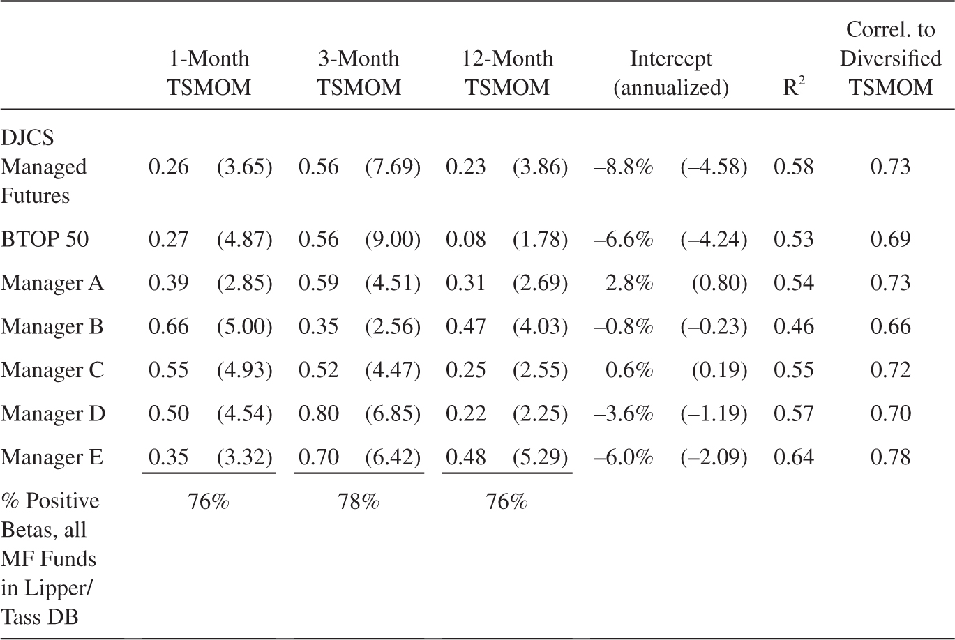
Notes: Panel A shows the performance of managed futures indices and the five largest managed futures managers in the Lipper/Tass database as of June 2012. All numbers are annualized. The alpha is the intercept from a regression on the MCSI World stock index, Barclays Bond Index, and the GSCI commodities index. Panel B shows the multivariate regression of managed futures indices and managers on time series momentum returns by trend horizon. T-statistics are reported in parentheses. The bottom row reports the percentage of all funds in the Lipper/Tass database with positive coefficients. The right-most column reports the correlation between the managed futures returns and the diversified TSMOM strategy.
Source: Hurst, Ooi, and Pedersen (2013).
Fees make a significant difference, given that most CTAs and managed futures hedge funds have historically charged at least 2% management fees and 20% performance fees. While we cannot know the exact before-fee manager returns, we can simulate the hypothetical fee for the time series momentum strategy. With a 2-and-20 fee structure, the average fee is around 6% per year for the diversified TSMOM strategy, although this high fee is due to the high simulated performance of the strategy. Furthermore, transaction costs are on the order of 1 to 4% per year for a sophisticated manager, possibly much higher for less sophisticated managers, and higher historically. Hence, after these estimated fees and transaction costs, the Sharpe ratio of the diversified time series momentum strategy would historically have been near 1, still comparing well to the indices and managers, but we note that historical transaction costs are not known and are associated with significant uncertainty.
Rather than comparing the performance of the time series momentum strategy to those of the indices and managers, we want to show that time series momentum can explain the strong performance of managed futures managers. To explain managed futures returns, we regress the returns of managed futures indices and managers  on the returns of 1-month, 3-month, and 12-month time series momentum:
![]()
Panel B of table 12.2 reports the results of these regressions. We see the time series momentum strategies explain the managed futures index and manager returns to a large extent in the sense that the R-squares of these regressions are large, ranging between 0.46 and 0.64. The table also reports the correlation of the managed futures indices and managers with the diversified TSMOM strategy. These correlations are large, ranging from 0.66 to 0.78, which provides another indication that time series momentum can explain the managed futures universe.
The intercepts reported indicate the excess returns (or alphas) after controlling for time series momentum. While the alphas relative to the traditional asset classes in Panel A were significantly positive, almost all the alphas relative to time series momentum in Panel B are negative. Even though the returns of the largest managers are biased to be high (due to the ex post selection of the managers), time series momentum nevertheless drives these alphas to be negative. This is another expression in which time series momentum can explain the managed futures space and is an illustration of the importance of fees and transaction costs. Another interesting finding that arises from Panel B is the relative importance of short-, medium-, and long-term trends for managed futures funds.
In summary, while many managed futures funds pursue many other types of strategies besides time series momentum, our results show that time series momentum explains the average alpha in the industry and a significant fraction of the time variation of returns.
12.6. IMPLEMENTATION: HOW TO MANAGE MANAGED FUTURES
We have seen that time series momentum can explain managed futures returns. In fact, this relatively simple strategy has realized a higher Sharpe ratio than most managers, at least on paper. This result suggests that fees and other implementation issues are important for the real-world success of these strategies. Indeed, as mentioned above, we estimate that a 2-and-20 fee structure implies a 6% average annual fee on the diversified time series momentum strategy run at a 10% annualized volatility. Other important implementation issues include transaction costs, rebalance methodology, margin requirements, and risk management.
To analyze the effect of how often the portfolio is rebalanced, figure 12.5 shows the gross Sharpe ratio for each trend horizon and the diversified time series momentum strategy as a function of rebalancing frequency. Daily and weekly rebalancing perform similarly, while the performance trails off with monthly and quarterly rebalancing frequencies. Naturally, the performance falls more quickly for the short- and medium-term strategies as these signals change more quickly, leading to a larger alpha decay.
As mentioned, the annual transaction costs of a managed futures strategy are typically about 1 to 4% for a sophisticated trader, possibly much higher for less sophisticated traders, and higher historically given higher transaction costs in the past. Transaction costs depend on a number of things. Transaction costs increase with rebalance frequency if the portfolio is mechanically rebalanced without transaction-cost optimization (although more frequent access to the market can also be used to source more liquidity) and transaction costs are higher for short-term trend signals than long-term trends. Hence, larger managers—for whom transaction costs play a more important role—may allocate a larger weight to medium- and long-term trend signals and relatively lower weight to short-term signals.
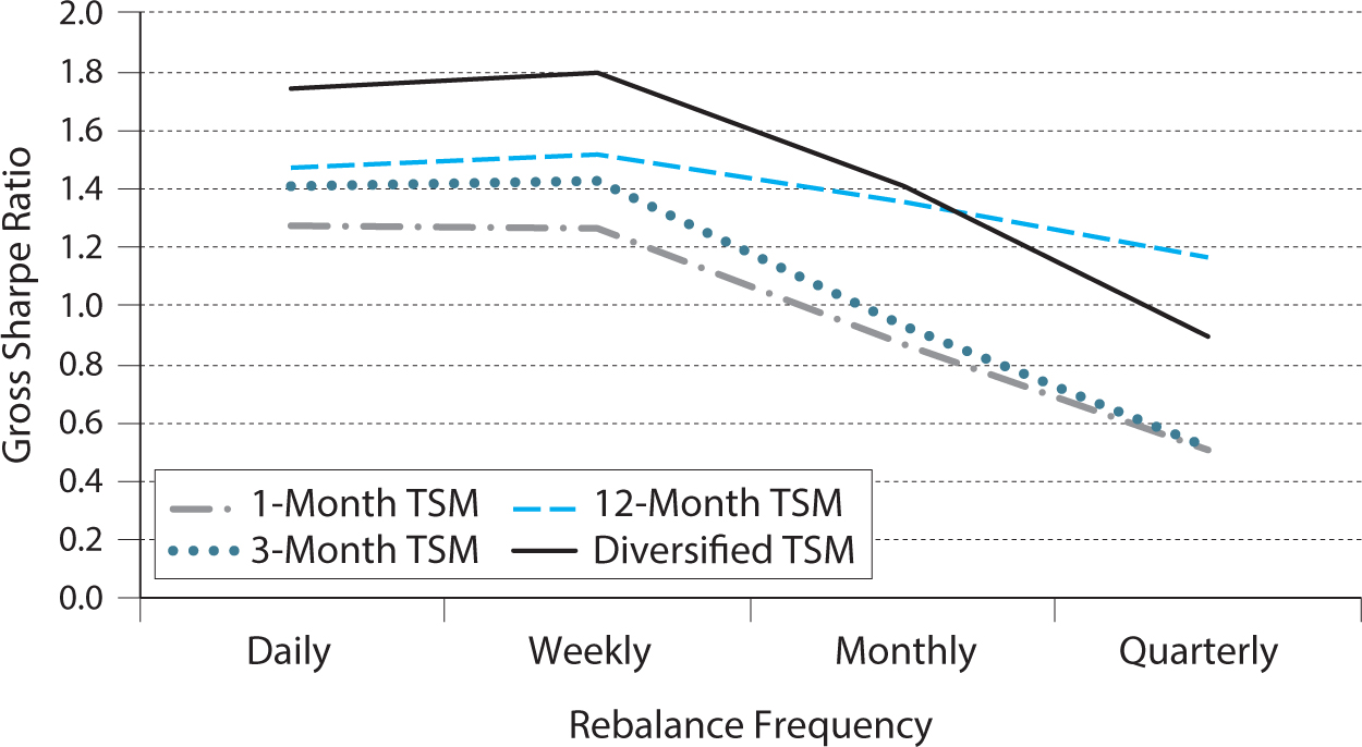
Figure 12.5. Gross Sharpe ratios at different rebalance frequencies.
This figure shows the Sharpe ratios gross of transaction costs of the 1-month, 3-month, 12-month, and diversified time series momentum strategies as a function of the rebalancing frequency.
To implement managed futures strategies, managers must post margin to counterparties, namely the futures commission merchant and the currency intermediation agent (or currency prime broker). The time series momentum strategy would typically have margin requirements of 8–12% for a large institutional investor and more than double that for a smaller investor. Hence, time series momentum is certainly implementable from a funding liquidity standpoint as it has a significant amount of free cash.
Risk management is the final implementation issue that we discuss. Our construction of trading strategies is systematic and already has built-in risk controls due to our constant-volatility methodology. This position sizing controls the risk of each security by scaling down the position when risk spikes up. Furthermore, it achieves a risk-balanced diversification across securities at all times. Lastly, some managed futures managers use drawdown control, further seek to identify overextended trends to limit the losses from sharp trend reversals, and try to identify short-term countertrends to improve performance in range-bound markets.
12.7. INTERVIEW WITH DAVID HARDING OF WINTON CAPITAL MANAGEMENT
David W. Harding is the chairman and chief executive officer of Winton Capital Management, a global investment manager focusing on managed futures investments. Before founding Winton Capital, Harding co-founded Adam Harding and Lueck (AHL) in 1987, one of the first systematic trend-following CTAs in Europe, which was subsequently bought by the Man Group and remains one of the cornerstones of the FTSE-listed company.
LHP: How did you become interested in managed futures investment in the first place?
DWH: I started at a stockbroker called Wood Mackenzie in London in 1982 after leaving Cambridge with a degree in natural sciences, specializing in theoretical physics. I was a trainee in the fixed interest area, and within the first month of my starting, the London Financial Futures Exchange—LIFFE—started. The first contracts on LIFFE were bond futures, so I took the opportunity to be posted onto the floor of the exchange. This way, I got interested in futures and charting and applying statistical programming to futures at the beginning of my career, when I was 21 years old.
LHP: How did you decide that you wanted to apply statistical techniques to that market, as opposed to what other people were doing at the time?
DWH: I was looking at long strings of numbers going up and down and drawing charts. I was trained as a scientist, and I had learned a lot in my physics degree about methods of analyzing data—for example, Fourier analysis—and I couldn’t help but wonder if this could be applied to these time series.
LHP: Is there a specific incident that set the course for your career?
DWH: I spent two years in the mid- ’80s drawing charts by hand every day, which is a very laborious process. That certainly gave me a lot of time to look at time series. When you press a button on your computer and a chart appears, you don’t interact with the data in a very detailed way. Whereas if you draw these graphs day by day by hand, you reflect on the empirical nature of the data more deeply. So, I would say that period I had at Sabre Fund Management had a big impact on my feeling about the non-randomness of the data.
LHP: Was there a particular property of the charts that caught your attention?
DWH: Trends. Trends are what you’re looking for. Trends are what technical analysis exists to try to foretell and forecast. People see trends in the data because there are trends in the data, and people are reasonably good at seeing trends in the data.
LHP: Can you talk about your investment process? How is it today, and how did you get there?
DWH: We study data about markets and look for evidence in the data for when the odds of the market moving up or down aren’t exactly 50/50. We place bets when the odds are in our favor.
LHP: You determine whether the odds are not 50/50 through extensive research and then trade through a systematic process, correct?
DWH: Yes, exactly. We trade in lots of markets at the same time, putting positions on and taking them off. It’s all coded into a computer program because it’s a more complicated pattern than any individual trader can manage.
LHP: What are the pros and cons of model-driven investment versus trading on someone’s instincts or a human’s assessment based on softer pieces of information?
DWH: The pro is intellectual rigor, discipline. It’s an evidence-based approach, so you’re demanding fairly hard-edged scientific evidence before risking money.
The main disadvantage, I would say, is that you can’t take into account all factors. If something’s never happened before, then your research can’t tell you anything about it.
LHP: Does your research suggest that it’s better to have the same type of model for every instrument, or is it better to have a very specific model for each one?
DWH: If you have very different models for very different markets, then you encounter problems with overfitting of data.
LHP: Do you think these opportunities arise because traders make systematic errors that are similar across all the different markets?
DWH: I’ll answer that in an oblique way by saying there is a theory, much beloved of academics, that markets are efficient, and that they perfectly discount all future information.
In its most extreme form, it says not only that markets discount the future, but they accurately reflect all fundamentals of economies and everything that’s known about companies and so on and so forth, and they synthesize this information into completely perfect prices.
This theory would be laughable if it wasn’t so widely believed in. It’s come out of valuing options and modeling diffusion processes: price movement as a diffusion using the Brownian motion and the heat equation. That is a good approximation for modeling short-term options, but to extend that to the idea that there is this perfect matrix of prices that reflects everything perfectly is putting too much weight on a small base of evidence, as they say in science.
LHP: So how do your models exploit that markets are not perfectly efficient?
DWH: Markets are social institutions and reflect all sorts of phenomena that you’d expect such social institutions to reflect. They reflect certain things about the price formation process, and one of those is, obviously, the tendency of markets to serially correlate because ideas catch on slowly and spread, and fevers develop and people get over-optimistic and become disappointed.
LHP: Are there some circumstances or events that illustrate the value of managed futures?
DWH: We tend to make money out of surprises, and people are very bad at foreseeing surprises. If you just look at the history of the last hundred years, I mean, the First World War came out of a clear, blue sky. Talk about the efficient market theory. Bond yields and stock prices didn’t move on July 25th, 1914, or July 23rd, 1914, despite the assassination of Franz Ferdinand a month before. They had no idea what was going to come. So the market didn’t efficiently discount the First World War. Then we had the Communist Revolution in Russia—efficient market theory didn’t get that. Same with the Second World War, Hitler, the arms race, the invention of computers. It’s just been one thing after another in terms of completely surprising the markets—and I’m not even touching on the last 20 years, the collapse of the banking system, and so on.
LHP: So how do managed futures or trend following benefit from surprises?
DWH: There are obviously large surprises in human history, continually. But there are also small surprises which affect one market.
LHP: But for an investor to benefit from a surprise, it cannot be a complete surprise; it would have to show up in prices before it happened; that is, it would have to unfold gradually.
DWH: Well, I guess that you’re right. Luckily, most surprises do unfold gradually. To preserve the ridiculous idea of efficient market theory, all surprises would have to be instantaneously discounted, but this is just not possible. The collapse of the banking system unfolded with a sickening series of events over time, so the stock market fell by 50% over the space of a year, and trend-following systems worked well.
LHP: Yes. Do you think that trend-following investment tends to push a price toward the fundamental or away from it?
DWH: I don’t think it’s really very easy to pin down the fundamental value of something. The idea of fundamentals suggests that there is an equilibrium price at which the market will clear. But, of course, the world isn’t in equilibrium. It’s changing all the time, isn’t it? You shouldn’t really say there’s a fundamental value, but a spectrum of possible fundamental values, and trend following probably moves prices around within the range of possible values.
LHP: Do you think that having more managed futures investors will tend to eliminate trends, or make trends stronger?
DWH: I can only give you an unsatisfactory answer, which is I think it’d probably change the autocorrelation spectrum of price data. In other words, it will change the nature of trends, somewhat.
LHP: Some people say that managed futures have tail-hedging properties. Do you agree?
DWH: I’m relatively uncomfortable with that concept. Over the last 20 years commodity trading advisors have tended to do well when stock markets go down. But CTAs can have a strong positive correlation to the stock market at some times and a strong negative correlation at others because the biggest sector they trade is stock indices. If there happens to be a substantial decline in stocks when we happen to be long, then we won’t have tail hedging properties at all. We’ll have tail exacerbating properties.
The best diversification you get from investing in a CTA is investing with somebody who doesn’t have a view about the future. And since most investment consists of people telling you what their view about the future is, it’s a novel idea to invest with somebody who doesn’t have a view about the future.
LHP: How important is it to keep changing one’s investment approach and continuing to do research?
DWH: There are no final and immutable truths in financial markets. If you think you’ve found the answer and all you have to do is implement it forever, then you are ultimately doomed. To be competitive, you’ve got to work hard and keep at it and keep going all the time.
LHP: Nevertheless, are there certain signals or parts of your model that you’ve implemented that you sort of came up with in the ’80s and you still use today?
DWH: Yeah, definitely there are. Because we trade relatively slowly, our models are not in a state of perpetual revolution. We’re changing things gradually and doing long-term research, which leads to, perhaps, more changes in the models as the years pass.
LHP: When you allocate to different asset classes, is that also based solely on research or is there any judgment in whether you put more weight on commodities versus equities, and so on?
DWH: It’s more or less a research question, but there is no uniquely accurate answer. A lot of our research gives very imprecise answers, in contrast to what people think. But you have a set of expected returns, a set of variance matrices, a set of transaction costs, and there is obviously some way in which to turn those into some sort of an optimal portfolio.
LHP: You’ve said that trend following is an “agnostic” form of investment—can you explain what you mean?
DWH: Yes. Trend following contains many less embedded assumptions than other types of investments. We don’t take a view on what’s going to happen next year and the year after and the year after. We don’t take a view on whether China is going to boom or bust. For example, we don’t take a view on whether there’s going to be an ongoing scarcity of commodities. There are people very busily setting up their portfolios with the absolute certainty that there’s going to be a terrific scarcity of commodities over the next 10 or 20 years, because it’s so obvious to them that, you know, the number of people is increasing, blah, blah, blah. But they weren’t doing that 10 years ago. In other words, they do it after prices have already risen for 10 years. I’d have a lot of respect for them if they’d done it before prices had risen for 10 years. That is a rather weak form of trend following. It’s trend following by accident.
A lot of what goes on in the investment world is fighting yesterday’s battles.
___________________
1 Ricardo’s trading rules are discussed by Grant (1838), and the quote attributed to Livermore is from Lefèvre (1923).
2 This chapter is based closely on Hurst, Ooi, and Pedersen (2013), “Demystifying Managed Futures,” Journal of Investment Management 11(3), 42–58. I thank my co-authors Brian Hurst and Yao Hua Ooi for their collaboration. The time series momentum methodology largely follows Moskowitz, Ooi, and Pedersen (2012) and is related to cross-sectional momentum, discussed in chapters 9 (quantitative equity) and 11 (global macro). See Fung and Hsieh (2001) for an early contribution on the characteristics of CTAs, Baltas and Kosowski (2013) for further analysis of CTAs in light of time series momentum, and Hurst, Ooi, and Pedersen (2014) for more than a century of evidence on time series momentum.
3 References are: i. Edwards (1968), Tversky and Kahneman (1974), and Barberis, Shleifer, and Vishny (1998); ii. Shefrin and Statman (1985) and Frazzini (2006); iii. Silber (1994); and iv. Mitchell, Pedersen, and Pulvino (2007) and Duffie (2010).
4 References are for i. Bikhchandani, Hirshleifer, and Welch (1992), De Long, Shleifer, Summers, and Waldmann (1990), Graham (1999), Hong and Stein (1999), and Welch (2000); ii. Wason (1960), Tversky and Kahneman (1974), and Daniel, Hirshleifer, Subrahmanyam (1998); iii. Vayanos and Woolley (2013).
5 Such long-run reversal exists for time series momentum strategies (Moskowitz, Ooi, and Pedersen 2012) and also in the cross section of equities (De Bondt and Thaler 1985) and the cross section of global asset classes (Asness, Moskowitz, and Pedersen 2013).
6 Our position sizes are chosen to target a constant volatility for each instrument following the methodology of Moskowitz, Ooi, and Pedersen (2012). More generally, one could consider strategies that vary the size of the position based on the strength of the estimated trend. For example, for intermediate price moves, one could take a small position or no position and increase the position depending on the magnitude of the price move.
7 These index returns are available at the following websites: http://www.barclayhedge.com/research/indices/btop/index.html; http://www.hedgeindex.com/hedgeindex/secure/en/indexperformance.aspx?cy=USD&indexname=HEDG_MGFUT