Chapter 3
Examining Samples

1. 3.1 Chapter Summary
2. 3.2 Glossary
3. 3.3 Equations
4. 3.4 Examples
5. 3.5 Exercises

Chapter Summary

In Chapter 3, we learned how to draw inferences about the population by examining a sample's observations. There are two processes that we can use. The first of these is estimation. In the process of estimation, the goal is to guess about the value of a parameter in the population. There are two kinds of estimates we use. One of those is a point estimate. A point estimate is a single number that is our best guess at the value of the parameter. The problem with point estimates is that they have a very low chance of being exactly equal to the population's parameter. This is because there are so many possible values that the probability for any single value is close to zero.

The other kind of estimate is an interval estimate, which is also known as a confidence interval. It differs from a point estimate in that an interval estimate implies that the population's parameter lies within an interval of values. The width of an interval estimate determines the level of confidence we can have that the population's parameter is included in the interval. The most commonly used interval estimate gives us 95% confidence that the parameter is included. In addition to the selected level of confidence, the width of an interval estimate is affected by the precision with which we can estimate the parameter. The greater the precision, the narrower the interval.

The second process we can use to draw inferences about the population by examining a sample is statistical hypothesis testing. In statistical hypothesis testing, we begin with a hypothesis that makes a specific statement about the population. This hypothesis is called the null hypothesis. It is so named because a specific statement that has a relevant biologic interpretation usually says that nothing is different. The next step is to take a sample from the population. It is important to note, in statistical hypothesis testing, the hypothesis comes before the data are collected.

Most of the “work” in statistical hypothesis testing involves calculations necessary to determine the P-value. A P-value is a conditional probability. The conditional event is getting a sample at least as different from what the null hypothesis states as the sample we observed. The conditioning event is that the null hypothesis is true. It is important not to get these events interchanged. A P-value does not tell us the probability that the null hypothesis is true. Instead, the P-value assumes that it is true.

The final step in hypothesis testing is deciding what to conclude. Our conclusion depends on how the numeric magnitude of the P-value compares to some preselected value called alpha (α). The most usual value of alpha is 0.05. If the P-value is less than or equal to alpha, we reject the null hypothesis. That is to say, we conclude that the null hypothesis is not a true statement about the population.

When we reject the null hypothesis, we automatically accept the alternative hypothesis as true. The alternative hypothesis is not tested. It is considered to be true whenever the null hypothesis is considered to be false. For this to work, the null and alternative hypotheses must cover all possibilities for the population. Keeping this in mind is important when choosing between a two-sided (in which differences from the null hypothesis can occur in both directions) and a one-sided (in which differences from the null hypothesis can occur in only one direction) alternative hypothesis. Most often, two-sided alternative hypotheses are the appropriate choice.

There are two kinds of errors that can be made in hypothesis testing. A type I error occurs when the null hypothesis is rejected but it is, in fact, true. The chance of making a type I error is determined by the choice of the value of alpha. If alpha is equal to 0.05, there is a 0.05 chance of making a type I error. A type II error occurs when the null hypothesis is accepted as true but it is, in fact, false. We do not know the probability of making a type II error, since the alternative hypothesis does not make a specific statement about the population. Because we do not know the chance of making a type II error, we avoid any opportunity for this type of error to occur. We do this by refusing to conclude that the null hypothesis is true. When the P-value is larger than alpha, we do not accept the null hypothesis as being true. Instead, we refrain from drawing a conclusion about the null hypothesis. This is often referred to as “failing to reject” the null hypothesis.

Both interval estimation and hypothesis testing take into account the role of chance in selecting a sample from the population. In Chapter 2, we considered this role of chance in selecting an individual from the population by using the distribution of data. When we are taking the role of chance on the entire sample, we use a different distribution. This distribution is called the sampling distribution. It is the distribution of estimates from all possible samples of a given size.

An important feature of the sampling distribution is that is tends to be a Gaussian distribution, even if the distribution of data is not a Gaussian distribution. This is especially true of sampling distributions of estimates of parameters of location from larger samples. This principle is called the central limit theorem. It is because of the central limit theorem that many of the statistical procedures commonly used in analyzing health research data are based on Gaussian distributions.

The parameters of the sampling distribution are related to the parameters of the distribution of data. The means of the two distributions are equal to the same value. This will always be the case for any unbiased estimate. An unbiased estimate is equal to the population's parameter, on the average. This is reflected in the sampling distribution by having the mean equal to the parameter that is being estimated (i.e., mean of the distribution of data).

The variances and standard deviations of the sampling distribution and distribution of data are related, but not equal to the same value. The sampling distribution is less dispersed than is the distribution of data. The reason for this is that the impact of extreme data values in a sample is offset by less extreme data values. Thus, estimates of the mean have less variation than do the data. How much less, depends on the number of observations in the sample. The greater the number of observations, the less variable the estimates. To emphasize the difference in dispersion between the sampling distribution and the distribution of data, the standard deviation of the sampling distribution is usually called the standard error.

Both interval estimation and hypothesis testing use the sampling distribution to take into account the role of chance in selecting a sample from the population. In hypothesis testing, it is the sampling distribution that is used to calculate a P-value. In interval estimation, it is the standard error of the sampling distribution that is used to represent the precision with which the parameter has been estimated. Although these sound like different processes, they are really just mirror images of the same logical procedure. If a null hypothesis is rejected, the null value will be outside the limits of the confidence interval.¹ If the null value is inside the confidence interval, the null hypothesis would not be rejected. This relationship allows us to use confidence intervals to test null hypotheses.

Glossary

1. Alpha (α) – in statistical hypothesis testing, alpha is the probability of making a type I error, because it is the value that the P-value must be equal to or less than to reject the null hypothesis. In interval estimation, alpha is the complement of the level of confidence we have that the population's parameter is included in the confidence interval.
2. Alternative Hypothesis – a statement concerning the population that must be true if the null hypothesis is not true. The alternative hypothesis and the null hypothesis are a collectively exhaustive set of possibilities for the population. In other words, one of those two hypotheses must be true.
3. Beta (β) – in statistical hypothesis testing, beta is the probability of making a type II error.
4. Central Limit Theorem – the statement that sampling distributions for estimates of parameters of location (such as the mean) tend to be Gaussian distributions, even if the data do not come from a Gaussian distribution. This tendency is greater for larger samples.
5. Confidence Interval – see Interval Estimate.
6. Degrees of Freedom – when used in calculation of an estimate of variance, degrees of freedom are the amount of information a sample contains to make the estimate.
7. Estimate – a value calculated from the sample's observations as a guess at the value of the population's parameter. See Point Estimate, Interval Estimate.
8. Estimation – the process of calculating a guess at the value of a parameter in the population from the observations in a sample.
9. Hypothesis testing – a process of drawing inferences about the population based on an examination of the sample's observations. Statistical hypothesis testing is a deductive process that begins with the formation of the null hypothesis and draws a conclusion based on the likelihood that the sample came from a population in which the null hypothesis was true.
10. Interval Estimate – an interval of values within which there is a good chance (most often, a 95% chance) that the population's value occurs. Synonym: Confidence Interval.
11. Null Hypothesis – a specific statement about the population that is tested in statistical hypothesis testing.
12. Null Value – the value of the population's parameter according to the null hypothesis.
13. One-Sided – when chance is taken into account by considering only one tail of the sampling distribution. A one-sided confidence interval has a finite limit in only one direction (i.e., above or below the point estimate). A one-sided alternative hypothesis considers possibilities in only one direction (i.e., either above or below the null value). Synonym: One-tailed.
14. P-value – the probability of getting a sample at least as far from the null value as is the sample's estimate given that the null hypothesis is true. The P-value is calculated as part of statistical hypothesis testing. It is compared to alpha to decide whether or not to reject the null hypothesis.
15. Point Estimate – a single value calculated from the sample's observations that is the best guess at the value of a parameter in the population.
16. Sample – a subset of the data from a population that we examine in an attempt to describe the population.
17. Sampling Distribution – the theoretical distribution of estimates that would be observed if all possible samples of a given size were selected from the population. It is the sampling distribution that is used to take into account the influence of chance on an estimate.
18. Standard Error – the standard deviation of a sampling distribution.
19. Statistically Significant – the result of statistical hypothesis testing is said to be statistically significant if the null hypothesis can be rejected.
20. Two-sided – when chance is taken into account by considering both tails of the sampling distribution. A two-sided confidence interval has finite limits in both directions (i.e., above and below the point estimate). A two-sided alternative hypothesis considers possibilities in both directions (i.e., above and below the null value). Synonym: Two-tailed.
21. Type I Error – mistakenly rejecting a true null hypothesis.
22. Type II Error – mistakenly accepting a false null hypothesis.
23. Unbiased – the property of a method of estimation in which the estimates from repeated samples are equal to the population's parameter, on the average.

Equations

$\mu \stackrel{\wedge}{=}\overline{Y}=\frac{\sum Y_i}{n}$	sample's point estimate of the mean of the distribution of data in the population. (see Equation {3.2})
${\sigma }^2\stackrel{\wedge}{=}{s}^2=\frac{\sum {(Y_i-\overline{Y})}^2}{n-1}$	sample's point estimate of the variance of the distribution of data in the population. (see Equation {3.4})
$s=\sqrt{s^2}$	sample's point estimate of the standard deviation of the distribution of data in the population. (see Example 3-1)
${\mu }_{\overline{Y}}=\mu \stackrel{\wedge}{=}\overline{Y}$	sample's point estimate of the mean of the sampling distribution for estimates of the mean. (see Equation {3.5})
${\sigma }_{\overline{Y}}^2=\frac{{\sigma }^2}{n}\stackrel{\wedge}{=}\frac{s^2}{n}$	sample's point estimate of the variance of the sampling distribution for estimates of the mean (the square of the standard error). (see Equation {3.6})
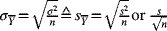${\sigma }_{\overline{Y}}=\sqrt{\frac{{\sigma }^2}{n}}\stackrel{\wedge}{=}{s}_{\overline{Y}}=\sqrt{\frac{s^2}{n}}\text{or}\frac{s}{\sqrt{n}}$	sample's point estimate of the standard error (i.e., the standard deviation of the sampling distribution) for estimates of the mean. (see Equation {3.7})
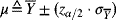$\mu \stackrel{\wedge}{=}\overline{Y}\pm (z_{\alpha /2}·{\sigma }_{\overline{Y}})$	sample's interval estimate (i.e., confidence interval) of the mean of the distribution of data in the population. (see Equation {3.8})
$z=\frac{\overline{Y}-{\mu }_0}{{\sigma }_{\overline{Y}}}$	conversion of the sample's estimate of the mean to a standard normal deviate (i.e., z-value). (see Equation {3.10})

Examples

In Chapter 2, we were interested in birth weights of infants in a particular population in which the mean birth weight is equal to 2,900 grams and the variance of birth weights is equal to 250,000 grams². Now, suppose we take a sample of 10 births from that population and observe the following results:

Table 3.1 Birth weights for a sample of 10 births.

	$Y$	$Y-\overline{Y}$	${(Y-\overline{Y})}^2$
	2,950	−7	49
	3,010	53	2,809
	2,895	−62	3,844
	3,110	153	23,409
	3,055	98	9,604
	3,185	228	51,984
	3,000	43	1,849
	2,660	−297	88,209
	2,945	−12	144
	2,760	−197	38,809
TOTAL	29,570	0	220,710

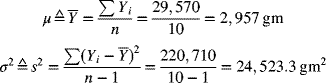
3.1. Calculate the sample's estimates of the mean and variance of birth weights in the population.

Most of the work in calculating these by hand has been done for us. We have the sum of the data values for calculation of the mean and the sum of squares for calculation of the variance.

$$\begin{array}{c}\hfill \mu \stackrel{\wedge}{=}\overline{Y}=\frac{\sum Y_i}{n}=\frac{\mathrm{29,570}}{10}=\mathrm{2,957}\text{gm}\hfill \\ \hfill {\sigma }^2\stackrel{\wedge}{=}{s}^2=\frac{\sum (Y_i-\overline{Y}{)}^2}{n-1}=\frac{\mathrm{220,710}}{10-1}=\mathrm{24,523.3}\mathrm{g}{\mathrm{m}}^2\hfill \end{array}$$

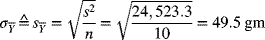
3.2. Calculate the sample's estimate of the standard error.

The sample's estimate of the standard error of the mean is calculated from the sample's estimate of the variance as follows:

$${\sigma }_{\overline{Y}}\stackrel{\wedge}{=}{s}_{\overline{Y}}=\sqrt{\frac{s^2}{n}}=\sqrt{\frac{\mathrm{24,523.3}}{10}}=49.5\text{gm}$$

3.3. Use Excel to estimate the mean, variance, and standard error. How do these compare to the answers to the first two examples?

To obtain estimates of the mean, variance, and standard error, we use the “Descriptive Statistics” analysis tool in “Data Analysis” under the “Data” tab.

The mean, variance, and standard error are the same as the rounded values we got when calculating these values by hand.

Now, suppose the population's standard error is equal to the sample's estimate (${\sigma }_{\overline{Y}}=s_{\overline{Y}}$).

3.4. Calculate a 95%, two-sided, confidence interval for the mean birth weight in this population.

To calculate a 95%, two-sided confidence interval for the mean, we need the point estimate of the mean and the standard error. We also need a z-value from Table B.1 to represent 95% confidence split between the tails of the standard normal distribution. That z-value is equal to 1.96.

$$\mu \stackrel{\wedge}{=}\overline{Y}\pm (z_{\alpha /2}·{\sigma }_{\overline{Y}})=\mathrm{2,957}\pm (1.96·49.5)=\mathrm{2,859.9}\text{to}\mathrm{3,054.1}$$

3.5. Use Excel to calculate a 95%, two-sided, confidence interval for the mean birth weight in the population. How does this interval compare to the answer to the previous example?

We can get the information we need for the confidence interval from the “Descriptive Statistics” analysis tool in “Data Analysis.” In that output, we are given a number labeled as “Confidence Level (95.0%).” To obtain a 95% confidence interval, we add and subtract this value from the point estimate of the mean. The limits of that confidence interval are 2,845.0 and 3,069. This is a wider confidence interval than the one we calculated in the previous example. The difference between these confidence intervals will be the subject of Chapter 4.

Suppose we wonder if this population is actually a sample from a larger population in which the mean birth weight is equal to 3,000 grams. To address this possibility, we could test the null hypothesis that the mean birth weight in the population from which this sample was taken is equal to 3,000 grams.

3.6. What would be the appropriate alternative hypothesis?

The null hypothesis is the mean in the population is equal to 3,000 gm. The alternative hypothesis must hypothesize that the mean in the population is equal to any other possible value, except the value in the null hypothesis. There is no reason to believe there are impossible values, so the alternative hypothesis is that the mean is not equal to 3,000 gm.

3.7. Test that null hypothesis while allowing a 5% chance of rejecting the null hypothesis if that null hypothesis was true.

To test the null hypothesis that the mean birth weight in the population is equal to 3,000 gm, we convert the observed mean to a standard normal deviate.²

$$z=\frac{\mathrm{2,957}-\mathrm{3,000}}{49.5}=-0.87$$

To obtain the P-value, we look up −0.87 in Table B.1. In that table, we learn a standard normal deviate of −0.87 corresponds to a probability of 0.1922 in each tail of the standard normal distribution. Thus, the P-value is two times 0.1922 or 0.3844. Since this P-value is greater than 0.05, we fail to reject the null hypothesis (i.e., we remain inconclusive).

3.8. How could you have tested that null hypothesis using the confidence interval from a previous example?

An easier way to test the null hypothesis that the mean birth weight is equal to 3,000 gm in the population, if we have a confidence interval, is to determine whether the null value (3,000 gm) is included within or excluded from the confidence interval (2,859.9 to 3,054.1). Since the null value is included in this interval, we fail to reject the null hypothesis.

Exercises

3.1. Suppose we were to take a sample of 10 births from a given population and determine the gestational ages (in days) at birth. Imagine that we observe the following results: 266, 267, 256, 259, 261, 255, 270, 271, 269, 266. Create an Excel dataset using those observations. What is the point estimate of the mean gestational age in the population from which this sample was drawn?

1. 220
2. 225
3. 255
4. 264
5. 306

3.2. Suppose we were to take a sample of 10 births from a given population and determine the gestational ages (in days) at birth. Imagine that we observe the following results: 266, 267, 256, 259, 261, 255, 270, 271, 269, 266. Create an Excel dataset using those observations. What is the sample's estimate of the standard deviation of gestational age in the population from which this sample was drawn?

1. 2.6
2. 3.1
3. 3.4
4. 4.3
5. 5.8

3.3. Suppose we are interested in diastolic blood pressure (dbp) among persons in a particular population. To investigate this, we take a sample of 9 persons from the population and measure their dbp. Imagine we obtain the following results 75, 80, 81, 72, 85, 88, 91, 87, 88. Create an Excel dataset using those observations. Which of the following is closest to the sample's estimate of the variance of diastolic blood pressure values?

1. 6.4
2. 17.5
3. 41.5
4. 74.7
5. 83.0

3.4. Suppose we take a sample of 36 persons from a particular population and measure their body weight. Then, we give each person a one-month's supply of appetite suppressants. At the end of the month, we weigh each person again and subtract their new weight from their first weight. Suppose we observe a mean difference in weight equal to 10 kg and we know the variance of differences in weight in the population is equal to 900 kg². Which of the following is closest to the interval of values within which we have 95% confidence that the population's mean lies?

1. 0.0 to 20.0
2. 0.2 to 19.8
3. 2.3 to 17.7
4. 5.0 to 15.0
5. 8.0 to 12.0

3.5. Suppose we were to conduct a study in which 16 persons with hypothyroidism were given two medications in a random order. In this study, we measure TSH (thyroid stimulating hormone) after the participants had taken each of the medications for a week. Suppose we observe that the mean difference in TSH levels was equal to 20 mg/dL and we know the standard deviation of differences between TSH levels is equal to 60 mg/dL in the population. Which of the following is closest to the value that reflects the precision with which we will be able to estimate the mean from that sample's observations (i.e., the standard error)?

1. 1.9
2. 3.7
3. 5.0
4. 7.7
5. 15.0

3.6. Suppose we were to conduct a study in which 16 persons with hypothyroidism were given two medications in a random order. In this study, we measure TSH after the participants had taken each of the medications for a week. Suppose we estimate the mean difference in TSH levels to be equal to 20 mg/dL and we estimate the standard deviation of differences between TSH levels to be equal to 60 mg/dL. What is the best null hypothesis to test about the mean difference in the population?

1. μ = 0
2. μ > 0
3. μ < 0
4. μ ≠ 0
5. μ = ?

3.7. Suppose we were to conduct a study in which 16 persons with hypothyroidism were given two medications in a random order. In this study, we measure TSH after the participants had taken each of the medications for a week. Suppose we estimate the mean difference in TSH levels to be equal to 20 mg/dL and we estimate the standard deviation of differences between TSH levels to be equal to 60 mg/dL. What is the best alternative hypothesis to consider about the mean difference in the population?

1. μ = 0
2. μ > 0
3. μ < 0
4. μ ≠ 0
5. μ = ?

3.8. Suppose we were to conduct a study in which 16 persons with hypothyroidism were given two medications in a random order. In this study, we measure TSH after the participants had taken each of the medications for a week. Suppose we estimate the mean difference in TSH levels to be equal to 20 mg/dL and we estimate the standard deviation of differences between TSH levels to be equal to 60 mg/dL. Test the appropriate null hypothesis allowing a 5% chance of making a type I error. Which of the following is the best conclusion to draw?

1. Reject the null hypothesis
2. Accept the null hypothesis
3. Fail to reject the null hypothesis
4. Fail to accept the null hypothesis
5. Hypothesis testing is not appropriate for these data

3.9. Suppose we take a sample of 36 persons from a particular population and measure their body weight. Then, we give each person a one-month's supply of appetite suppressants. At the end of the month, we weigh each person again and subtract their new weight from their first weight. Suppose we observe a mean difference in weight equal to 10 kg and calculate a 95% confidence interval for the estimate that ranges from 0.2 kg to 19.8 kg. Which of the following are the best null and alternative hypotheses to test about the mean difference in the population?

1. H₀: μ = 0 and H_A: μ = 0
2. H₀: μ ≠ 0 and H_A: μ = 0
3. H₀: μ = 0 and H_A: μ ≠ 0
4. H₀: μ = 0 and H_A: μ > 0
5. H₀: μ = 0 and H_A: μ < 0

3.10. Suppose we take a sample of 36 persons from a particular population and measure their body weight. Then, we give each person a one-month's supply of appetite suppressants. At the end of the month, we weigh each person again and subtract their new weight from their first weight. Suppose we observe a mean difference in weight equal to 10 kg and calculate a 95% confidence interval for that estimate that ranges from 0.2 kg to 19.8 kg. Which of the following is the best conclusion to draw if we were to test the null hypothesis that the mean difference in weight is equal to zero in the population?

1. Reject both the null and alternative hypotheses
2. Accept both the null and alternative null hypotheses
3. Reject the null hypothesis and accept the alternative hypothesis
4. Accept the null hypothesis and reject the alternative hypothesis
5. It is best not to draw a conclusion about the null and alternative hypotheses from these observations

Notes

1. Being exactly equal to the limit of a confidence interval is considered to be outside the interval.

2. We will learn a better method in Chapter 4.