Chapter 7
Summarizing It All
IN THIS CHAPTER
 Working with things great and small
Understanding symmetry, peaks, and plateaus
Experiencing special moments
Finding frequencies
Getting descriptive
The measures of central tendency and variability that I discuss in earlier chapters aren’t the only ways of summarizing a set of scores. These measures are a subset of descriptive statistics. Some descriptive statistics — like maximum, minimum, and range — are easy to understand. Some — like skewness and kurtosis — are not.
This chapter covers descriptive statistics and shows you how to calculate them in R.
How Many?
Perhaps the fundamental descriptive statistic is the number of scores in a set of data. In earlier chapters, I work with length(), the R function that calculates this number. As in earlier chapters, I work with the Cars93 data frame, which is in the MASS package. (If it isn’t selected, click the check box next to MASS on the Packages tab.)
Cars93 holds data on 27 variables for 93 cars available in 1993. What happens when you apply length() to the data frame?
> length(Cars93)
[1] 27
So length() returns the number of variables in the data frame. The function ncol() does the same thing:
> ncol(Cars93)
[1] 27
I already know the number of cases (rows) in the data frame, but if I had to find that number, nrow() would get it done:
> nrow(Cars93)
[1] 93
If you want to know how many cases in the data frame meet a particular condition — like how many cars originated in the USA — you have to take into account the way R treats conditions: R attaches the label “TRUE” to cases that meet a condition, and “FALSE” to cases that don’t. Also, R assigns the value 1 to “TRUE” and 0 to “FALSE.”
To count the number of USA-originated cars, then, you state the condition and then add up all the 1s:
> sum(Cars93$Origin == "USA")
[1] 48
To count the number of non-USA cars in the data frame, you can change the condition to “non-USA”, of course, or you can use != — the “not equal to” operator:
> sum(Cars93$Origin != "USA")
[1] 45
More complex conditions are possible. For the number of 4-cylinder USA cars:
> sum(Cars93$Origin == "USA" & Cars93$Cylinders == 4)
[1] 22
Or, if you prefer no $-signs:
> with(Cars93, sum(Origin == "USA" & Cylinders == 4))
[1] 22
To calculate the number of elements in a vector, length(), as you may have read earlier, is the function to use. Here is a vector of horsepowers for 4-cylinder USA cars:
> Horsepower.USA.Four <- Cars93$Horsepower[Origin ==
          "USA" & Cylinders == 4]
and here’s the number of horsepower values in that vector:
> length(Horsepower.USA.Four)
[1] 22
The High and the Low
Two descriptive statistics that need no introduction are the maximum and minimum value in a set of scores:
> max(Horsepower.USA.Four)
[1] 155
> min(Horsepower.USA.Four)
[1] 63
If you happen to need both values at the same time:
> range(Horsepower.USA.Four)
[1] 63 155
Living in the Moments
In statistics, moments are quantities that are related to the shape of a set of numbers. By “shape of a set of numbers,” I mean “what a histogram based on the numbers looks like” — how spread out it is, how symmetric it is, and more.
A raw moment of order k is the average of all numbers in the set, with each number raised to the kth power before you average it. So the first raw moment is the arithmetic mean. The second raw moment is the average of the squared scores. The third raw moment is the average of the cubed scores, and so on.
A central moment is based on the average of deviations of numbers from their mean. (Beginning to sound vaguely familiar?) If you square the deviations before you average them, you have the second central moment. If you cube the deviations before you average them, that’s the third central moment. Raise each one to the fourth power before you average them, and you have the fourth central moment. I could go on and on, but you get the idea.
Two quick questions: 1. For any set of numbers, what’s the first central moment? 2. By what other name do you know the second central moment?
Two quick answers: 1. Zero. 2. Population variance. Reread Chapter 5 if you don’t believe me.
A teachable moment
Before I proceed, I think it’s a good idea to translate into R everything I’ve said so far in this chapter. That way, when you get to the next R package to install (which calculates moments), you’ll know what’s going on behind the scenes.
Here’s a function for calculating a central moment of a vector:
cen.mom <-function(x,y){mean((x - mean(x))^y)}
The first argument, x, is the vector. The second argument, y, is the order (second, third, fourth …).
Here’s a vector to try it out on:
Horsepower.USA <- Cars93$Horsepower[Origin == "USA"]
And here are the second, third, and fourth central moments:
> cen.mom(Horsepower.USA,2)
[1] 2903.541
> cen.mom(Horsepower.USA,3)
[1] 177269.5
> cen.mom(Horsepower.USA,4)
[1] 37127741
Back to descriptives
What does all this about moments have to do with descriptive statistics? As I said … well … a moment ago, think of a histogram based on a set of numbers. The first raw moment (the mean) locates the center of the histogram. The second central moment indicates the spread of the histogram. The third central moment is involved in the symmetry of the histogram, which is called skewness. The fourth central moment figures into how fat or thin the tails (extreme ends) of the histogram are. This is called kurtosis. Getting into moments of higher order than that is way beyond the scope of this book.
But let’s get into symmetry and “tailedness.”
Skewness
Figure 7-1 shows three histograms. The first is symmetric; the other two are not. The symmetry and the asymmetry are reflected in the skewness statistic.
For the symmetric histogram, the skewness is 0. For the second histogram — the one that tails off to the right — the value of the skewness statistic is positive. It's also said to be “skewed to the right.” For the third histogram (which tails off to the left), the value of the skewness statistic is negative. It's also said to be “skewed to the left.”
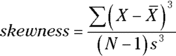
Now for a formula. I’ll let Mk represent the kth central moment. To calculate skewness, it’s
In English, the skewness of a set of numbers is the third central moment divided by the second central moment raised to the three-halves power. With the R function I defined earlier, it’s easier done than said:
> cen.mom(Horsepower.USA,3)/cen.mom(Horsepower.USA,2)^1.5
[1] 1.133031
With the moments package, it’s easier still. On the Packages tab, click Install and type moments into the Install Packages dialog box, and click Install. Then on the Packages tab, click the check box next to moments.
Here’s its skewness() function in action:
> skewness(Horsepower.USA)
[1] 1.133031
So the skew is positive. How does that compare with the horsepower for non-USA cars?
> Horsepower.NonUSA <- Cars93$Horsepower[Origin == "non-USA"]
> skewness(Horsepower.NonUSA)
[1] 0.642995
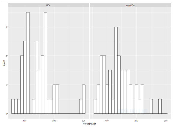
The skew is more positive for USA cars than for non-USA cars. What do the two histograms look like?
I produced them side-by-side in Figure 4-1, over in Chapter 4. For convenience, I show them here as Figure 7-2.
The code that produces them is
ggplot(Cars93, aes(x=Horsepower)) +
geom_histogram(color="black", fill="white",binwidth = 10)+
facet_wrap(~Origin)
Consistent with the skewness values, the histograms show that in the USA cars, the scores are more bunched up on the left than they are in the non-USA cars.
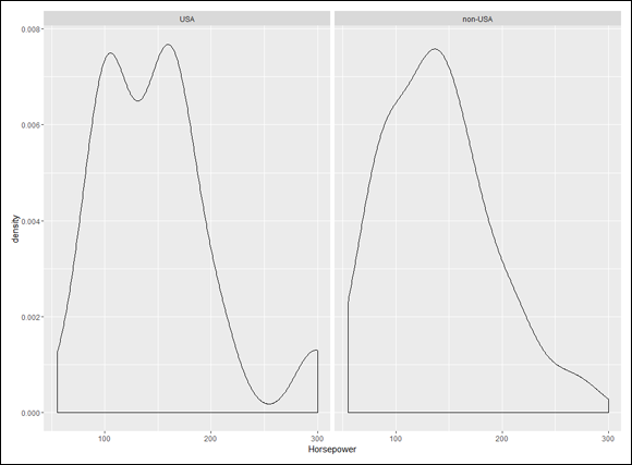
It’s sometimes easier to see trends in a density plot rather than in a histogram. A density plot shows the proportions of scores between a given lower boundary and a given upper boundary (like the proportion of cars with horsepower between 100 and 140). I discuss density in more detail in Chapter 8.
Changing one line of code produces the density plots:
ggplot(Cars93, aes(x=Horsepower)) +
geom_density() +
facet_wrap(~Origin)
Figure 7-3 shows the two density plots.
With the density plots, it seems to be easier (for me, anyway) to see the more leftward tilt (and hence, more positive skew) in the plot on the left.
Kurtosis
Figure 7-4 shows two histograms. The first has fatter tails than the second. The first is said to be leptokurtic. The second is platykurtic. The kurtosis for the first histogram is greater than for the second.
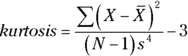
The formula for kurtosis is
where M4 is the fourth central moment and M2 is the second central moment. So kurtosis is the fourth central moment divided by the square of the second central moment.
 Many statisticians subtract 3 from the result of the kurtosis formula. They refer to that value as excess kurtosis. By “excess,” they mean kurtosis that’s greater (or possibly less) than the kurtosis of something called the standard normal distribution, which I discuss in Chapter 8. Because of the subtraction, excess kurtosis can be negative. Why does 3 represent the kurtosis of the standard normal distribution? Don’t ask.
Using the function I defined earlier, the kurtosis of horsepower for USA cars is
> cen.mom(Horsepower.USA,4)/cen.mom(Horsepower.USA,2)^2
[1] 4.403952
Of course, the kurtosis() function in the moments package makes this a snap:
> kurtosis(Horsepower.USA)
[1] 4.403952
The fatter tail in the left-side density plot in Figure 7-3 suggests that the USA cars have a higher kurtosis than the non-USA cars. Is this true?
> kurtosis(Horsepower.NonUSA)
[1] 3.097339
Yes, it is!
In addition to skewness() and kurtosis(), the moments package provides a function called moment() that does everything cen.mom() does and a bit more. I just thought it would be a good idea to show you a user-defined function that illustrates what goes into calculating a central moment. (Was I being “momentous” … or did I just “seize the moment”? Okay. I’ll stop.)
Tuning in the Frequency
A good way to explore data is to find out the frequencies of occurrence for each category of a nominal variable, and for each interval of a numerical variable.
Nominal variables: table() et al
For nominal variables, like Type of Automobile in Cars93, the easiest way to get the frequencies is the table() function I use earlier:
> car.types <-table(Cars93$Type)
> car.types
Compact Large Midsize Small Sporty Van
16 11 22 21 14 9
Another function, prop.table(), expresses these frequencies as proportions of the whole amount:
> prop.table(car.types)
Compact Large Midsize Small Sporty Van
0.17204301 0.11827957 0.23655914 0.22580645 0.15053763 0.09677419
 The values here appear out of whack because the page isn’t as wide as the Console window. If I round off the proportions to two decimal places, the output looks a lot better on the page:
> round(prop.table(car.types),2)
Compact Large Midsize Small Sporty Van
0.17 0.12 0.24 0.23 0.15 0.10
Another function, margin.table(), adds up the frequencies:
> margin.table(car.types)
[1] 93
Numerical variables: hist()
Tabulating frequencies for intervals of numerical data is part and parcel of creating histograms. (See Chapter 3.) To create a table of frequencies, use the graphic function hist(), which produces a list of components when the plot argument is FALSE:
> prices <- hist(Cars93$Price, plot=F, breaks=5)
> prices
$breaks
[1] 0 10 20 30 40 50 60 70
$counts
[1] 12 50 19 9 2 0 1
$density
[1] 0.012903226 0.053763441 0.020430108 0.009677419 0.002150538 0.000000000
[7] 0.001075269
$mids
[1] 5 15 25 35 45 55 65
$xname
[1] "Cars93$Price"
$equidist
[1] TRUE
(In Cars93, remember, each price is in thousands of dollars.)
Although I specified five breaks, hist() uses a number of breaks that makes everything look “prettier.” From here, I can use mids (the interval-midpoints) and counts to make a matrix of the frequencies, and then a data frame:
> prices.matrix <- matrix(c(prices$mids,prices$counts), ncol = 2)
> prices.frame <- data.frame(prices.matrix)
> colnames(prices.frame) <- c("Price Midpoint (X $1,000)","Frequency")
> prices.frame
Price Midpoint (X $1,000) Frequency
1 5 12
2 15 50
3 25 19
4 35 9
5 45 2
6 55 0
7 65 1
Cumulative frequency
Another way of looking at frequencies is to examine cumulative frequencies: Each interval’s cumulative frequency is the sum of its own frequency and all frequencies in the preceding intervals.
The cumsum() function does the arithmetic on the vector of frequencies:
> prices$counts
[1] 12 50 19 9 2 0 1
> cumsum(prices$counts)
[1] 12 62 81 90 92 92 93
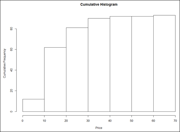
To plot a cumulative frequency histogram, I substitute the cumulative frequencies vector for the original one:
> prices$counts <- cumsum(prices$counts)
and then apply plot():
> plot(prices, main = "Cumulative Histogram", xlab = "Price", ylab = "Cumulative Frequency")
The result is Figure 7-5.
Step by step: The empirical cumulative distribution function
The empirical cumulative distribution function (ecdf) is closely related to cumulative frequency. Rather than show the frequency in an interval, however, the ecdf shows the proportion of scores that are less than or equal to each score. If this sounds familiar, it’s probably because you read about percentiles in Chapter 6.
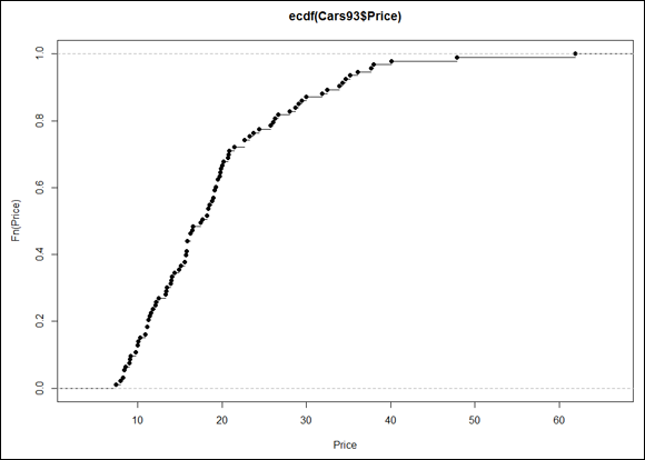
In base R, it’s easy to plot the ecdf:
> plot(ecdf(Cars93$Price), xlab = "Price", ylab = "Fn(Price)")
This produces Figure 7-6.
The uppercase F on the y-axis is a notational convention for a cumulative distribution. The Fn means, in effect, “cumulative function” as opposed to f or fn, which just means “function.” (The y-axis label could also be Percentile(Price).)
Look closely at the plot. When consecutive points are far apart (like the two on the top right), you can see a horizontal line extending rightward out of a point. (A line extends out of every point, but the lines aren’t visible when the points are bunched up.) Think of this line as a “step” and then the next dot is a step higher than the previous one. How much higher? That would be 1/N, where N is the number of scores in the sample. For Cars93, that would be 1/93, which rounds off to .011. (Now reconsider the title of this subsection. See what I did there?)
Why is this called an “empirical” cumulative distribution function? Something that’s empirical is based on observations, like sample data. Is it possible to have a non-empirical cumulative distribution function (cdf)? Yes — and that’s the cdf of the population that the sample comes from. (See Chapter 1.) One important use of the ecdf is as a tool for estimating the population cdf.
So the plotted ecdf is an estimate of the cdf for the population, and the estimate is based on the sample data. To create an estimate, you assign a probability to each point and then add up the probabilities, point by point, from the minimum value to the maximum value. This produces the cumulative probability for each point. The probability assigned to a sample value is the estimate of the proportion of times that value occurs in the population. What is the estimate? That’s the aforementioned 1/N for each point — .011, for this sample. For any given value, that might not be the exact proportion in the population. It’s just the best estimate from the sample.
I prefer to use ggplot() to visualize the ecdf. Because I base the plot on a vector (Cars93$Price), the data source is NULL:
ggplot(NULL, aes(x=Cars93$Price))
In keeping with the step-by-step nature of this function, the plot consists of steps, and the geom function is geom_step. The statistic that locates each step on the plot is the ecdf, so that’s
geom_step(stat="ecdf")
and I’ll label the axes:
labs(x= "Price X $1,000",y = "Fn(Price)")
Putting those three lines of code together
ggplot(NULL, aes(x=Cars93$Price)) +
geom_step(stat="ecdf") +
labs(x= "Price X $1,000",y = "Fn(Price)")
gives you Figure 7-7.
To put a little pizzazz in the graph, I add a dashed vertical line at each quartile. Before I add the geom function for a vertical line, I put the quartile information in a vector:
price.q <-quantile(Cars93$Price)
And now
geom_vline(aes(xintercept=price.q),linetype = "dashed")
adds the vertical lines. The aesthetic mapping sets the x-intercept of each line at a quartile value.
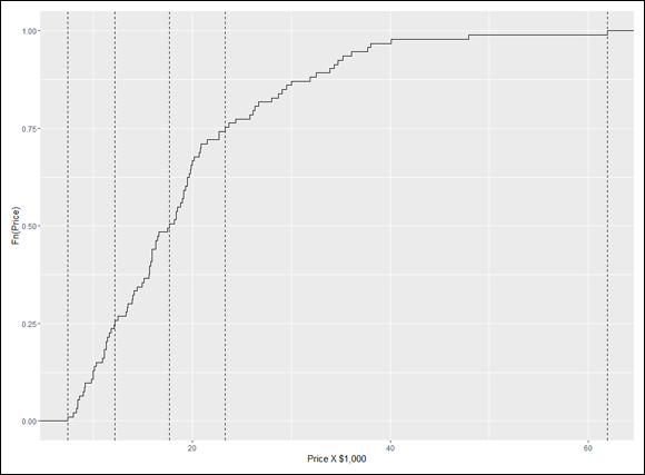
So these lines of code
ggplot(NULL, aes(x=Cars93$Price)) +
geom_step(stat="ecdf") +
labs(x= "Price X $1,000",y = "Fn(Price)") +
geom_vline(aes(xintercept=price.q),linetype = "dashed")
result in Figure 7-8.
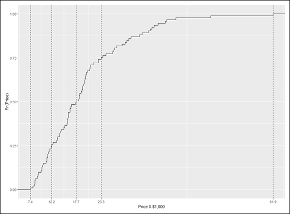
A nice finishing touch is to put the quartile-values on the x-axis. The function scale_x_continuous() gets that done. It uses one argument called breaks (which sets the location of values to put on the axis) and another called labels (which puts the values on those locations). Here’s where that price.q vector comes in handy:
scale_x_continuous(breaks = price.q,labels = price.q)
And here’s the R code that creates Figure 7-9:
ggplot(NULL, aes(x=Cars93$Price)) +
geom_step(stat="ecdf") +
labs(x= "Price X $1,000",y = "Fn(Price)") +
geom_vline(aes(xintercept=price.q),linetype = "dashed")+
scale_x_continuous(breaks = price.q,labels = price.q)
Numerical variables: stem()
Box plot creator John Tukey popularized the stem-and-leaf plot as a way to quickly visualize a distribution of numbers. It’s not a “plot” in the usual sense of a graph in the Plot window. Instead, it’s an arrangement of numbers in the Console window. With each score rounded off to the nearest whole number, each “leaf” is a score’s rightmost digit. Each “stem” consists of all the other digits.
An example will help. Here are the prices of the cars in Cars93, arranged in ascending order and rounded off to the nearest whole number (remember that each price is in thousands of dollars):
> rounded <- (round(sort(Cars93$Price),0))
I use cat() to display the rounded values on this page. (Otherwise, it would look like a mess.) The value of its fill argument limits the number of characters (including spaces) on each line:
> cat(rounded, fill = 50)
7 8 8 8 8 9 9 9 9 10 10 10 10 10 11 11 11 11 11
11 12 12 12 12 12 13 13 14 14 14 14 14 15 15 16
16 16 16 16 16 16 16 16 16 17 18 18 18 18 18 18
19 19 19 19 19 20 20 20 20 20 20 20 21 21 21 22
23 23 23 24 24 26 26 26 27 28 29 29 30 30 32 32
34 34 35 35 36 38 38 40 48 62
The stem() function produces a stem-and-leaf plot of these values:
> stem(Cars93$Price)
The decimal point is 1 digit(s) to the right of the |
0 | 788889999
1 | 00000111111222233344444556666666667788888999999
2 | 00000001112333446667899
3 | 00234455688
4 | 08
5 |
6 | 2
In each row, the number to the left of the vertical line is the stem. The remaining numbers are the leaves for that row. The message about the decimal point means “multiply each stem by 10.” Then add each leaf to that stem. So the bottom row tells you that one rounded score in the data is 62. The next row up reveals that no rounded score is between 50 and 59. The row above that one indicates that one score is 40 and another is 48. I’ll leave it to you to figure out (and verify) the rest.
 As I reviewed the leaves, I noticed that the stem plot shows one score of 32 and another of 33. By contrast, the rounded scores show two 32s and no 33s. Apparently, stem() rounds differently than round() does.
Summarizing a Data Frame
If you’re looking for descriptive statistics for the variables in a data frame, the summary() function will find them for you. I illustrate with a subset of the Cars93 data frame:
> autos <- subset(Cars93, select = c(MPG.city,Type, Cylinders, Price, Horsepower))
> summary(autos)
MPG.city Type Cylinders Price
Min. :15.00 Compact:16 3 : 3 Min. : 7.40
1st Qu.:18.00 Large :11 4 :49 1st Qu.:12.20
Median :21.00 Midsize:22 5 : 2 Median :17.70
Mean :22.37 Small :21 6 :31 Mean :19.51
3rd Qu.:25.00 Sporty :14 8 : 7 3rd Qu.:23.30
Max. :46.00 Van : 9 rotary: 1 Max. :61.90
Horsepower
Min. : 55.0
1st Qu.:103.0
Median :140.0
Mean :143.8
3rd Qu.:170.0
Max. :300.0
Notice the maxima, minima, and quartiles for the numerical variables and the frequency tables for Type and for Cylinders.
Two functions from the Hmisc package also summarize data frames. To use these functions, you need Hmisc in your library. (On the Packages tab, click Install and type Hmisc into the Packages box in the Install dialog box. Then click Install.)
One function, describe.data.frame(), provides output that’s a bit more extensive than what you get from summary():
> describe.data.frame(autos)
autos
5 Variables 93 Observations
-------------------------------------------------------------
MPG.city
n missing unique Info Mean .05 .10
93 0 21 0.99 22.37 16.6 17.0
.25 .50 .75 .90 .95
18.0 21.0 25.0 29.0 31.4
lowest : 15 16 17 18 19, highest: 32 33 39 42 46
-------------------------------------------------------------
Type
n missing unique
93 0 6
Compact Large Midsize Small Sporty Van
Frequency 16 11 22 21 14 9
% 17 12 24 23 15 10
-------------------------------------------------------------
Cylinders
n missing unique
93 0 6
3 4 5 6 8 rotary
Frequency 3 49 2 31 7 1
% 3 53 2 33 8 1
-------------------------------------------------------------
Price
n missing unique Info Mean .05 .10
93 0 81 1 19.51 8.52 9.84
.25 .50 .75 .90 .95
12.20 17.70 23.30 33.62 36.74
lowest : 7.4 8.0 8.3 8.4 8.6
highest: 37.7 38.0 40.1 47.9 61.9
-------------------------------------------------------------
Horsepower
n missing unique Info Mean .05 .10
93 0 57 1 143.8 78.2 86.0
.25 .50 .75 .90 .95
103.0 140.0 170.0 206.8 237.0
lowest : 55 63 70 73 74, highest: 225 255 278 295 300
-------------------------------------------------------------
A value labeled Info appears in the summaries of the numerical variables. That value is related to the number of tied scores — the greater the number of ties, the lower the value of Info. (The calculation of the value is fairly complicated.)
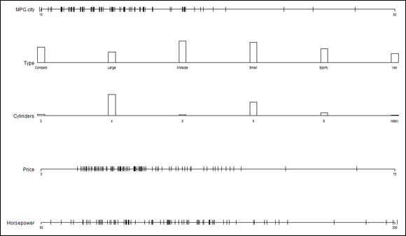
Another Hmisc function, datadensity(), gives graphic summaries, as in Figure 7-10:
> datadensity(autos)
If you plan to use the datadensity() function, arrange for the first data frame variable to be numerical. If the first variable is categorical (and thus appears at the top of the chart), longer bars in its plot are cut off at the top.