The Levi-Civita Connection

If we are to use geodesics and covariant derivatives as tools for studying Riemannian geometry, it is evident that we need a way to single out a particular connection on a Riemannian manifold that reflects the properties of the metric. In this chapter, guided by the example of the tangential connection on a submanifold of $\mathbb {R}^n$ , we describe two properties that determine a unique connection on every Riemannian manifold. The first property, compatibility with the metric, is easy to motivate and understand. The second, symmetry, is a bit more mysterious; but it is motivated by the fact that it is invariantly defined, and is always satisfied by the tangential connection. It turns out that these two conditions are enough to determine a unique connection associated with any Riemannian or pseudo-Riemannian metric, called the Levi-Civita connection after the early twentieth-century Italian differential geometer Tullio Levi-Civita.

After defining the Levi-Civita connection, we investigate the exponential map, which conveniently encodes the collective behavior of geodesics and allows us to study how they change as the initial point and initial velocity vary. Having established the properties of this map, we introduce normal neighborhoods and normal coordinates, which are essential computational and theoretical tools for studying local geometric properties near a point. Then we introduce the analogous notion for studying properties near a submanifold: tubular neighborhoods and Fermi coordinates. Finally, we return to our three main model Riemannian manifolds and determine their geodesics.

Except where noted otherwise, the results and proofs of this chapter do not use positivity of the metric, so they apply equally well to Riemannian and pseudo-Riemannian manifolds.

The Tangential Connection Revisited

We are eventually going to show that on each Riemannian manifold there is a natural connection that is particularly well suited to computations in Riemannian geometry. Since we get most of our intuition about Riemannian manifolds from studying submanifolds of $\mathbb {R}^n$ with the induced metric, let us start by examining that case.

Let $M\subseteq \mathbb {R}^n$ be an embedded submanifold. As a guiding principle, consider the idea mentioned at the beginning of Chapter 4: a geodesic in M should be “as straight as possible.” A reasonable way to make this rigorous is to require that the geodesic have no acceleration in directions tangent to the manifold, or in other words that its acceleration vector have zero orthogonal projection onto TM.

The tangential connection defined in Example 4.9 is perfectly suited to this task, because it computes covariant derivatives on M by taking ordinary derivatives in $\mathbb {R}^n$ and projecting them orthogonally to TM.

It is easy to compute covariant derivatives along curves in M with respect to the tangential connection. Suppose $\gamma :I\mathrel {\rightarrow }M$ is a smooth curve. Then $\gamma$ can be regarded as either a smooth curve in M or a smooth curve in $\mathbb {R}^n$ , and a smooth vector field V along $\gamma$ that takes its values in TM can be regarded as either a vector field along $\gamma$ in M or a vector field along $\gamma$ in $\mathbb {R}^n$ . Let $\bar{D}_t V$ denote the covariant derivative of V along $\gamma$ (as a curve in $\mathbb {R}^n$ ) with respect to the Euclidean connection $\bar{\nabla }$ , and let $D^\top _tV$ denote its covariant derivative along $\gamma$ (as a curve in M) with respect to the tangential connection $\nabla ^\top$ . The next proposition shows that the two covariant derivatives along $\gamma$ have a simple relationship to each other.

Proposition 5.1.

Let $M\subseteq \mathbb {R}^n$ be an embedded submanifold, $\gamma :I\mathrel {\rightarrow }M$ a smooth curve in M, and V a smooth vector field along $\gamma$ that takes its values in TM. Then for each $t\in I$ ,

$\begin{aligned} D_t^\top V(t) = \pi ^\top \big (\bar{D}_t V(t)\big ). \end{aligned}$

Proof.

Let $t_0\in I$ be arbitrary. By Proposition 2.14, on some neighborhood U of $\gamma (t_0)$ in $\mathbb {R}^n$ there is an adapted orthonormal frame for TM, that is, a local orthonormal frame $(E_1,\dots , E_n)$ for $T\mathbb {R}^n$ such that $(E_1,\dots , E_k)$ restricts to an orthonormal frame for TM at points of $M\cap U$ (where $k=\dim M$ ). If $\varepsilon >0$ is small enough that $\gamma \big ((t_0-\varepsilon , t_0+\varepsilon )\big )\subseteq U$ , then for $t\in (t_0-\varepsilon , t_0+\varepsilon )$ we can write

$\begin{aligned} V(t) = V^1(t) E_1\big |_{\gamma (t)} + \dots + V^k(t) E_k\big |_{\gamma (t)}, \end{aligned}$

for some smooth functions $V^1,\dots , V^k:(t_0-\varepsilon , t_0+\varepsilon )\mathrel {\rightarrow }\mathbb {R}$ . Formula (4.15) yields

$\begin{aligned} \pi ^\top \big ( \bar{D}_tV(t) \big )&= \pi ^\top \bigg (\sum _{i=1}^k \Big ( \dot{V}^i(t) E_i\big |_{\gamma (t)} + V^i(t) \bar{\nabla }_{\gamma '(t)} E_i\big |_{\gamma (t)} \Big )\bigg )\\&= \sum _{i=1}^k \Big ( \dot{V}^i(t) E_i\big |_{\gamma (t)} + V^i(t) \pi ^\top \big (\bar{\nabla }_{\gamma '(t)} E_i\big |_{\gamma (t)} \big )\Big )\\&= \sum _{i=1}^k \Big ( \dot{V}^i(t) E_i\big |_{\gamma (t)} + V^i(t) \nabla ^\top _{\gamma '(t)} E_i\big |_{\gamma (t)} \Big )\\&= D^\top _tV(t). \end{aligned}$

$\square$

Corollary 5.2.

Suppose $M\subseteq \mathbb {R}^n$ is an embedded submanifold. A smooth curve $\gamma :I\mathrel {\rightarrow }M$ is a geodesic with respect to the tangential connection on M if and only if its ordinary acceleration $\gamma ''(t)$ is orthogonal to $T_{\gamma (t)}M$ for all $t\in I$ .

Proof.

As noted in Example 4.8, the connection coefficients of the Euclidean connection on $\mathbb {R}^n$ are all zero. Thus it follows from (4.15) that the Euclidean covariant derivative of $\gamma '$ along $\gamma$ is just its ordinary acceleration: $\bar{D}_t\gamma '(t) = \gamma ''(t)$ . The corollary then follows from Proposition 5.1. $\square$

These considerations can be extended to pseudo-Riemannian manifolds as well. Let $\big (\mathbb {R}^{r,s},\bar{q}^{(r, s)}\big )$ be the pseudo-Euclidean space of signature (r, s). If $M\subseteq \mathbb {R}^{r, s}$ is an embedded Riemannian or pseudo-Riemannian submanifold, then for each $p\in M$ , the tangent space $T_p\mathbb {R}^{r, s}$ decomposes as a direct sum $T_pM \oplus N_pM$ , where $N_pM = (T_pM)^\perp$ is the orthogonal complement of $$T_pM$$

with respect to $\bar{q}^{(r, s)}$ . We let $\pi ^\top :T_p\mathbb {R}^{r, s}\mathrel {\rightarrow }T_pM$ be the $\bar{q}^{(r, s)}$ -orthogonal projection, and define the tangential connection $\nabla ^\top$ on M by

../images/56724_2_En_5_Chapter/56724_2_En_5_Equ86_HTML.png

where $\tilde{X}$ and $\tilde{Y}$ are smooth extensions of X and Y to a neighborhood of M, and $\bar{\nabla }$ is the ordinary Euclidean connection on $\mathbb {R}^{r, s}$ . This is a well-defined connection on M by the same argument as in the Euclidean case, and the next proposition is proved in exactly the same way as Corollary 5.2.

Proposition 5.3.

Suppose M is an embedded Riemannian or pseudo-Riemannian submanifold of the pseudo-Euclidean space $\mathbb {R}^{r, s}$ . A smooth curve $\gamma :I\mathrel {\rightarrow }M$ is a geodesic with respect to $\nabla ^\top$ if and only if $\gamma ''(t)$ is $\bar{q}^{(r, s)}$ -orthogonal to $T_{\gamma (t)}M$ for all $t\in I$ .

$\blacktriangleright$ Exercise 5.4. Prove the preceding proposition.

Connections on Abstract Riemannian Manifolds

There is a celebrated (and hard) theorem of John Nash [Nas56] that says that every Riemannian metric on a smooth manifold can be realized as the induced metric of some embedding in a Euclidean space. That theorem was later generalized independently by Robert Greene [Gre70] and Chris J. S. Clarke [Cla70] to pseudo-Riemannian metrics. Thus, in a certain sense, we would lose no generality by studying only submanifolds of Euclidean and pseudo-Euclidean spaces with their induced metrics, for which the tangential connection would suffice. However, when we are trying to understand intrinsic properties of a Riemannian manifold, an embedding introduces a great deal of extraneous information, and in some cases actually makes it harder to discern which geometric properties depend only on the metric. Our task in this chapter is to distinguish some important properties of the tangential connection that make sense for connections on an abstract Riemannian or pseudo-Riemannian manifold, and to use them to single out a unique connection in the abstract case.

Metric Connections

The Euclidean connection on $\mathbb {R}^n$ has one very nice property with respect to the Euclidean metric: it satisfies the product rule

$\begin{aligned} \bar{\nabla }_X\left\langle Y,Z \right\rangle = \left\langle \bar{\nabla }_XY, Z \right\rangle + \left\langle Y,\bar{\nabla }_XZ \right\rangle , \end{aligned}$

as you can verify easily by computing in terms of the standard basis. (In this formula, the left-hand side represents the covariant derivative of the real-valued function $\langle Y, Z \rangle$ regarded as a (0, 0)-tensor field, which is really just $X\langle Y, Z \rangle$ by virtue of property (ii) of Prop. 4.15.) The Euclidean connection has the same property with respect to the pseudo-Euclidean metric on $\mathbb {R}^{r, s}$ . It is almost immediate that the tangential connection on a Riemannian or pseudo-Riemannian submanifold satisfies the same product rule, if we now interpret all the vector fields as being tangent to M and interpret the inner products as being taken with respect to the induced metric on M (see Prop. 5.8 below).

This property makes sense on an abstract Riemannian or pseudo-Riemannian manifold. Let g be a Riemannian or pseudo-Riemannian metric on a smooth manifold M (with or without boundary). A connection $\nabla$ on TM is said to be compatible with $\varvec{g}$ , or to be a metric connection, if it satisfies the following product rule for all $X,Y, Z\in \mathfrak X(M)$ :

$\begin{aligned} \nabla _X\left\langle Y,Z \right\rangle = \left\langle \nabla _XY, Z \right\rangle +\left\langle Y,\nabla _XZ \right\rangle . \end{aligned}$

(5.1)

The next proposition gives several alternative characterizations of compatibility with a metric, any one of which could be used as the definition.

Proposition 5.5

(Characterizations of Metric Connections). Let (M, g) be a Riemannian or pseudo-Riemannian manifold (with or without boundary), and let $\nabla$ be a connection on TM. The following conditions are equivalent:

(a)
$\nabla$ is compatible with g: $\nabla _X\left\langle Y,Z \right\rangle = \left\langle \nabla _XY, Z \right\rangle +\left\langle Y,\nabla _XZ\right\rangle$ .
(b)
g is parallel with respect to $\nabla$ : $\nabla g\equiv 0$ .
(c)
In terms of any smooth local frame , the connection coefficients of $\nabla$ satisfy
$\begin{aligned} \Gamma _{ki}^l g_{lj} + \Gamma _{kj}^l g_{il} = E_k (g_{ij}). \end{aligned}$

(5.2)
(d)
If V, W are smooth vector fields along any smooth curve $\gamma$ , then
$\begin{aligned} \frac{d}{dt}\langle V,W \rangle = \left\langle {D_tV}, W \right\rangle + \left\langle V,{D_tW} \right\rangle . \end{aligned}$

(5.3)
(e)
If V, W are parallel vector fields along a smooth curve $\gamma$ in M, then $\langle V, W \rangle$ is constant along $\gamma$ .
(f)
Given any smooth curve $\gamma$ in M, every parallel transport map along $\gamma$ is a linear isometry.
(g)
Given any smooth curve $\gamma$ in M, every orthonormal basis at a point of $\gamma$ can be extended to a parallel orthonormal frame along $\gamma$ (Fig. 5.1).

../images/56724_2_En_5_Chapter/56724_2_En_5_Fig1_HTML.png — Fig. 5.1:
A parallel orthonormal frame

Proof.

First we prove (a) $\Leftrightarrow$ (b). By (4.14) and (4.12), the total covariant derivative of the symmetric 2-tensor g is given by

$\begin{aligned} (\nabla g)(Y,Z,X) = (\nabla _X g)(Y,Z) = X(g(Y,Z)) - g(\nabla _X Y, Z) - g(Y,\nabla _X Z). \end{aligned}$

This is zero for all X, Y, Z if and only if (5.1) is satisfied for all X, Y, Z.

To prove (b) $\Leftrightarrow$ (c), note that Proposition 4.18 shows that the components of $\nabla g$ in terms of a smooth local frame $$(E_i)$$

are

$\begin{aligned} g_{ij;k} = E_k(g_{ij}) - \Gamma _{ki}^l g_{lj} - \Gamma _{kj}^l g_{il}. \end{aligned}$

These are all zero if and only if (5.2) is satisfied.

Next we prove (a) $\Leftrightarrow$ (d). Assume (a), and let V, W be smooth vector fields along a smooth curve $\gamma :I\mathrel {\rightarrow }M$ . Given $t_0\in I$ , in a neighborhood of $\gamma (t_0)$ we may choose coordinates $\left( x^i\right)$ and write $V=V^i\partial _i$ and $W=W^j\partial _j$ for some smooth functions $V^i, W^j:I\mathrel {\rightarrow }\mathbb {R}$ . Applying (5.1) to the extendible vector fields $\partial _i, \partial _j$ , we obtain

$\begin{aligned} \frac{d}{dt}\langle V, W \rangle&= \frac{d}{dt}\left( V^i W^j \langle \partial _i,\partial _j \rangle \right) \\&= \big (\dot{V}^i W^j + V^i \dot{W}^j\big ) \langle \partial _i,\partial _j \rangle + V^i W^j \big (\langle \nabla _{\gamma '(t)}\partial _i,\partial _j \rangle +\langle \partial _i,\nabla _{\gamma '(t)}\partial _j \rangle \big )\\&= \langle D_t V, W \rangle + \langle V, D_t W \rangle , \end{aligned}$

which proves (d). Conversely, if (d) holds, then in particular it holds for extendible vector fields along $\gamma$ , and then (a) follows from part (iii) of Theorem 4.24.

Now we will prove (d) $\Rightarrow$ (e) $\Rightarrow$ (f) $\Rightarrow$ (g) $\Rightarrow$ (d). Assume first that (d) holds. If V and W are parallel along $\gamma$ , then (5.3) shows that $\langle V, W \rangle$ has zero derivative with respect to t, so it is constant along $\gamma$ .

Now assume (e). Let $$v_0,w_0$$ be arbitrary vectors in $T_{\gamma (t_0)}M$ , and let V, W be their parallel transports along $\gamma$ , so that $$V(t_0)=v_0$$ , $$W(t_0)=w_0$$ , $P^\gamma _{t_0t_1}v_0 = V(t_1)$ , and $P^\gamma _{t_0t_1}w_0 = W(t_1)$ . Because $\langle V, W \rangle$ is constant along $\gamma$ , it follows that $\langle P^\gamma _{t_0t_1}v_0,P^\gamma _{t_0t_1}w_0 \rangle = \langle V(t_1), W(t_1) \rangle = \langle V(t_0), W(t_0) \rangle = \langle v_0,w_0 \rangle$ , so $P^\gamma _{t_0t_1}$ is a linear isometry.

Next, assuming (f), we suppose $\gamma :I\mathrel {\rightarrow }M$ is a smooth curve and $$(b_i)$$ is an orthonormal basis for $T_{\gamma (t_0)}M$ , for some $t_0\in I$ . We can extend each $$b_i$$ by parallel transport to obtain a smooth parallel vector field $$E_i$$ along $\gamma$ , and the assumption that parallel transport is a linear isometry guarantees that the resulting n-tuple $$(E_i)$$ is an orthonormal frame at all points of $\gamma$ .

Finally, assume that (g) holds, and let $$(E_i)$$

be a parallel orthonormal frame along $\gamma$ . Given smooth vector fields V and W along $\gamma$ , we can express them in terms of this frame as $$V=V^i E_i$$

and

. The fact that the frame is orthonormal means that the metric coefficients $g_{ij} = \langle E_i, E_j \rangle$ are constants along $\gamma$ ( $\pm 1$ or 0), and the fact that it is parallel means that $D_tV=\dot{V}^i E_i$ and $D_tW = \dot{W}^i E_i$ . Thus both sides of (5.3) reduce to the following expression:

$\begin{aligned} g_{ij}\big (\dot{V}^i W^j + V^i \dot{W}^j\big ). \end{aligned}$

(5.4)

This proves (d). $\square$

Corollary 5.6.

Suppose (M, g) is a Riemannian or pseudo-Riemannian manifold with or without boundary, $\nabla$ is a metric connection on M, and $\gamma :I\mathrel {\rightarrow }M$ is a smooth curve.

(a)
$|\gamma '(t)|$ is constant if and only if $D_t\gamma '(t)$ is orthogonal to $\gamma '(t)$ for all $t\in I$ .
(b)
If $\gamma$ is a geodesic, then $|\gamma '(t)|$ is constant.

$\blacktriangleright$ Exercise 5.7. Prove the preceding corollary.

Proposition 5.8.

If M is an embedded Riemannian or pseudo-Riemannian submanifold of $\mathbb {R}^n$ or $\mathbb {R}^{r, s}$ , the tangential connection on M is compatible with the induced Riemannian or pseudo-Riemannian metric.

Proof.

We will show that $\nabla ^\top$ satisfies (5.1). Suppose $X,Y, Z\in \mathfrak X(M)$ , and let $\tilde{X},\tilde{Y},\tilde{Z}$ be smooth extensions of them to an open subset of $\mathbb {R}^n$ or $\mathbb {R}^{r, s}$ . At points of M, we have

$\begin{aligned} \nabla _X^\top \langle Y,Z \rangle&= X\langle Y,Z \rangle = \tilde{X}\big \langle \tilde{Y},\tilde{Z}\big \rangle \\&= \bar{\nabla }_{\tilde{X}}\big \langle \tilde{Y},\tilde{Z}\big \rangle \\&= \big \langle \bar{\nabla }_{\tilde{X}} \tilde{Y},\tilde{Z}\big \rangle + \big \langle \tilde{Y}, \bar{\nabla }_{\tilde{X}} \tilde{Z}\big \rangle \\&= \big \langle \pi ^\top \big (\bar{\nabla }_{\tilde{X}} \tilde{Y}\big ), \tilde{Z}\big \rangle + \big \langle \tilde{Y}, \pi ^\top \big (\bar{\nabla }_{\tilde{X}} \tilde{Z}\big )\big \rangle \\&= \big \langle \nabla ^\top _X Y, Z\big \rangle + \big \langle Y, \nabla ^\top _X Z\big \rangle , \end{aligned}$

where the next-to-last equality follows from the fact that $\tilde{Z}$ and $\tilde{Y}$ are tangent to M. $\square$

Symmetric Connections

It turns out that every abstract Riemannian or pseudo-Riemannian manifold admits many different metric connections (see Problem 5-1), so requiring compatibility with the metric is not sufficient to pin down a unique connection on such a manifold. To do so, we turn to another key property of the tangential connection. Recall the definition (4.3) of the Euclidean connection. The expression on the right-hand side of that definition is reminiscent of part of the coordinate expression for the Lie bracket:

$\begin{aligned}{}[X, Y] = X\big (Y^i\big )\frac{\partial }{\partial x^i}- Y\big (X^i\big )\frac{\partial }{\partial x^i}. \end{aligned}$

In fact, the two terms in the Lie bracket formula are exactly the coordinate expressions for $\bar{\nabla }_X Y$ and $\bar{\nabla }_Y X$ . Therefore, the Euclidean connection satisfies the following identity for all smooth vector fields X, Y:

$\begin{aligned} \bar{\nabla }_X Y - \bar{\nabla }_Y X = [X, Y]. \end{aligned}$

This expression has the virtue that it is coordinate-independent and makes sense for every connection on the tangent bundle. We say that a connection $\nabla$ on the tangent bundle of a smooth manifold M is symmetric if

$\begin{aligned} \nabla _X Y - \nabla _Y X \equiv [X,Y] \text { for all } X, Y\in \mathfrak X(M). \end{aligned}$

The symmetry condition can also be expressed in terms of the torsion tensor of the connection, which was introduced in Problem 4-6; this is the smooth (1, 2)-tensor field $\tau :\mathfrak X(M)\times \mathfrak X(M)\mathrel {\rightarrow }\mathfrak X(M)$ defined by

$\begin{aligned} \tau (X,Y)= \nabla _X Y - \nabla _Y X - [X, Y]. \end{aligned}$

Thus a connection $\nabla$ is symmetric if and only if its torsion vanishes identically. It follows from the result of Problem 4-6 that a connection is symmetric if and only if its connection coefficients in every coordinate frame satisfy $\Gamma ^k_{ij} = \Gamma ^k_{ji}$ ; this is the origin of the term “symmetric."

Proposition 5.9.

If M is an embedded (pseudo-)Riemannian submanifold of a (pseudo-)Euclidean space, then the tangential connection on M is symmetric.

Proof.

Let M be an embedded Riemannian or pseudo-Riemannian submanifold of $\mathbb {R}^n$ , where $\mathbb {R}^n$ is endowed either with the Euclidean metric or with a pseudo-Euclidean metric $\bar{q}^{(r, s)}$ , $$r+s=n$$

. Let $X, Y\in \mathfrak X(M)$ , and let $\tilde{X},\tilde{Y}$ be smooth extensions of them to an open subset of the ambient space. If $\iota :M\mathrel {\hookrightarrow }\mathbb {R}^n$ represents the inclusion map, it follows that X and Y are $\iota$ -related to $\tilde{X}$ and $\tilde{Y}$ , respectively, and thus by the naturality of the Lie bracket (Prop. A.39), [X, Y] is $\iota$ -related to $\big [\tilde{X},\tilde{Y}\big ]$ . In particular, $\big [\tilde{X},\tilde{Y}\big ]$ is tangent to M, and its restriction to M is equal to [X, Y]. Therefore,

$\begin{aligned} \nabla ^\top _X Y - \nabla ^\top _Y X&= \pi ^\top \big (\bar{\nabla }_{\tilde{X}}\tilde{Y}\big |_M - \bar{\nabla }_{\tilde{Y}}\tilde{X}\big |_M\big )\\&= \pi ^\top \big ( \bigl [ \tilde{X},\tilde{Y}\bigr ]\big |_M\big )\\&= \bigl [ \tilde{X},\tilde{Y}\bigr ]\big |_M\\&=[X, Y]. \end{aligned}$

$\square$

The last two propositions show that if we wish to single out a connection on each Riemannian or pseudo-Riemannian manifold in such a way that it matches the tangential connection when the manifold is presented as an embedded submanifold of $\mathbb {R}^n$ or $\mathbb {R}^{r, s}$ with the induced metric, then we must require at least that the connection be compatible with the metric and symmetric. It is a pleasant fact that these two conditions are enough to determine a unique connection.

Theorem 5.10

(Fundamental Theorem of Riemannian Geometry). Let (M, g) be a Riemannian or pseudo-Riemannian manifold (with or without boundary). There exists a unique connection $\nabla$ on TM that is compatible with g and symmetric. It is called the Levi-Civita connection of ${\varvec{g}}$ (or also, when g is positive definite, the Riemannian connection ).

Proof.

We prove uniqueness first, by deriving a formula for $\nabla$ . Suppose, therefore, that $\nabla$ is such a connection, and let $X,Y, Z\in \mathfrak X(M)$ . Writing the compatibility equation three times with X, Y, Z cyclically permuted, we obtain

$\begin{aligned} \begin{aligned} X\langle Y,Z \rangle&= \langle \nabla _XY,Z \rangle +\langle Y,\nabla _XZ \rangle ,\\ Y\langle Z,X \rangle&= \langle \nabla _YZ,X \rangle +\langle Z,\nabla _YX \rangle ,\\ Z\langle X,Y \rangle&= \langle \nabla _ZX, Y \rangle +\langle X,\nabla _ZY \rangle . \end{aligned} \end{aligned}$

Using the symmetry condition on the last term in each line, this can be rewritten as

$\begin{aligned} \begin{aligned} X\langle Y,Z \rangle&= \langle \nabla _XY,Z \rangle +\langle Y,\nabla _ZX \rangle +\langle Y,[X,Z] \rangle ,\\ Y\langle Z,X \rangle&= \langle \nabla _YZ,X \rangle +\langle Z,\nabla _XY \rangle +\langle Z,[Y,X] \rangle ,\\ Z\langle X,Y \rangle&= \langle \nabla _ZX,Y \rangle +\langle X,\nabla _YZ \rangle +\langle X,[Z, Y] \rangle . \end{aligned} \end{aligned}$

Adding the first two of these equations and subtracting the third, we obtain

$\begin{aligned} \begin{aligned} X\langle Y,Z \rangle +Y\langle Z,X \rangle -&Z\langle X, Y \rangle =\\&2\langle \nabla _XY,Z \rangle +\langle Y,[X,Z] \rangle +\langle Z,[Y,X] \rangle -\langle X,[Z, Y] \rangle . \end{aligned} \end{aligned}$

Finally, solving for $\langle \nabla _XY, Z \rangle$ , we get

$\begin{aligned} \langle \nabla _XY, Z \rangle = \tfrac{1}{2}\big ( X\langle Y,Z \rangle&+Y\langle Z,X \rangle -Z\langle X,Y \rangle \nonumber \\&\qquad -\langle Y,[X,Z] \rangle -\langle Z,[Y,X] \rangle +\langle X,[Z, Y] \rangle \big ). \end{aligned}$

(5.5)

Now suppose $\nabla ^1$ and $\nabla ^2$ are two connections on TM that are symmetric and compatible with g. Since the right-hand side of (5.5) does not depend on the connection, it follows that $\langle \nabla ^1_XY-\nabla ^2_XY, Z \rangle =0$ for all X, Y, Z. This can happen only if $\nabla ^1_XY=\nabla ^2_XY$ for all X and Y, so $\nabla ^1=\nabla ^2$ .

To prove existence, we use (5.5), or rather a coordinate version of it. It suffices to prove that such a connection exists in each coordinate chart, for then uniqueness ensures that the connections in different charts agree where they overlap.

Let $\big (U,\big (x^i\big )\big )$ be any smooth local coordinate chart. Applying (5.5) to the coordinate vector fields, whose Lie brackets are zero, we obtain

$\begin{aligned} \left\langle \nabla _{\partial _{i}} \partial _{j} , \partial _{l} \right\rangle = \tfrac{1}{2} \bigl ( \partial _{i} \left\langle \partial _{j},\partial _{l}\right\rangle +\partial _{j} \left\langle \partial _{l},\partial _{i}\right\rangle -\partial _{l} \left\langle \partial _{i},\partial _{j}\right\rangle \bigr ). \end{aligned}$

(5.6)

Recall the definitions of the metric coefficients and the connection coefficients:

$\begin{aligned} g_{ij} = \left\langle \partial _{i},\partial _{j}\right\rangle ,\qquad \qquad \nabla _{\partial _{i}} \partial _{j} = \Gamma _{ij}^m \partial _{m}. \end{aligned}$

Inserting these into (5.6) yields

$\begin{aligned} \Gamma _{ij}^m g_{ml} = \tfrac{1}{2} \left( \partial _i g_{jl} + \partial _j g_{il} - \partial _l g_{ij}\right) . \end{aligned}$

(5.7)

Finally, multiplying both sides by the inverse matrix $g^{kl}$ and noting that $g_{ml}g^{kl}=\delta _m^k$ , we get

$\begin{aligned} \Gamma _{ij}^k= \tfrac{1}{2} g^{kl} \left( \partial _i g_{jl} + \partial _j g_{il} - \partial _l g_{ij}\right) . \end{aligned}$

(5.8)

This formula certainly defines a connection in each chart, and it is evident from the formula that $\Gamma _{ij}^k = \Gamma _{ji}^k$ , so the connection is symmetric by Problem 4-6(b). Thus only compatibility with the metric needs to be checked. Using (5.7) twice, we get

$\begin{aligned} \begin{aligned} \Gamma _{ki}^l g_{lj} + \Gamma _{kj}^l g_{il}&= \tfrac{1}{2} \left( \partial _k g_{ij} + \partial _i g_{kj} - \partial _j g_{ki} \right) + \tfrac{1}{2} \left( \partial _k g_{ji} + \partial _j g_{ki} - \partial _i g_{kj} \right) \\&= \partial _k g_{ij}. \end{aligned} \end{aligned}$

By Proposition 5.5(c), this shows that $\nabla$ is compatible with g. $\square$

A bonus of this proof is that it gives us explicit formulas that can be used for computing the Levi-Civita connection in various circumstances.

Corollary 5.11

(Formulas for the Levi-Civita Connection). Let (M, g) be a Riemannian or pseudo-Riemannian manifold (with or without boundary), and let $\nabla$ be its Levi-Civita connection.

(a)
In terms of vector fields: If X, Y, Z are smooth vector fields on M, then
$\begin{aligned} \langle \nabla _XY, Z \rangle = \tfrac{1}{2}&\big ( X\langle Y,Z \rangle +Y\langle Z,X \rangle -Z\langle X,Y \rangle \nonumber \\&\qquad \qquad -\langle Y,[X,Z] \rangle -\langle Z,[Y,X] \rangle +\langle X,[Z, Y] \rangle \big ). \end{aligned}$

(5.9)
(This is known as Koszul’s formula.)
(b)
In coordinates: In any smooth coordinate chart for M, the coefficients of the Levi-Civita connection are given by
$\begin{aligned} \Gamma _{ij}^k= \tfrac{1}{2} g^{kl} \left( \partial _i g_{jl} + \partial _j g_{il} - \partial _l g_{ij}\right) . \end{aligned}$

(5.10)
(c)
In a local frame: Let be a smooth local frame on an open subset $U\subseteq M$ , and let $c_{ij}^k:U\mathrel {\rightarrow }\mathbb {R}$ be the smooth functions defined by
$\begin{aligned}{}[E_i, E_j] = c_{ij}^k E_k. \end{aligned}$

(5.11)
Then the coefficients of the Levi-Civita connection in this frame are
$\begin{aligned} \Gamma _{ij}^k = \tfrac{1}{2} g^{kl}\big ( E_i g_{jl} + E_j g_{il} - E_l g_{ij} - g_{jm} c^m_{il} - g_{lm}c^m_{ji} + g_{im}c^m_{lj}\big ). \end{aligned}$

(5.12)
(d)
In a local orthonormal frame: If g is Riemannian, is a smooth local orthonormal frame, and the functions $c_{ij}^k$ are defined by (5.11), then
$\begin{aligned} \Gamma _{ij}^k = \tfrac{1}{2} \big ( c_{ij}^k - c_{ik}^j - c_{jk}^i\big ). \end{aligned}$

(5.13)

Proof.

We derived (5.9) and (5.10) in the proof of Theorem 5.10. To prove (5.12), apply formula (5.9) with $$X=E_i$$

, and

, to obtain

$\begin{aligned} \Gamma _{ij}^q g_{ql}&= \langle \nabla _{E_i}E_j, E_l \rangle \\&= \tfrac{1}{2}\bigl ( E_i g_{jl} + E_j g_{il} - E_l g_{ij} - g_{jm} c^m_{il} - g_{lm}c^m_{ji} + g_{im}c^m_{lj}\big ). \end{aligned}$

Multiplying both sides by $g^{kl}$ and simplifying yields (5.12). Finally, under the hypotheses of (d), we have $g_{ij} = \delta _{ij}$ , so (5.12) reduces to (5.13) after rearranging and using the fact that $c_{ij}^k$ is antisymmetric in i, j. $\square$

On every Riemannian or pseudo-Riemannian manifold, we will always use the Levi-Civita connection from now on without further comment. Geodesics with respect to this connection are called Riemannian (or pseudo-Riemannian ) geodesics, or simply “geodesics” as long as there is no risk of confusion. The connection coefficients $\Gamma _{ij}^k$ of the Levi-Civita connection in coordinates, given by (5.10), are called the Christoffel symbols of g.

The next proposition shows that these connections are familiar ones in the case of embedded submanifolds of Euclidean or pseudo-Euclidean spaces.

Proposition 5.12.

(a)
The Levi-Civita connection on a (pseudo-)Euclidean space is equal to the Euclidean connection.
(b)
Suppose M is an embedded (pseudo-)Riemannian submanifold of a (pseudo-)Euclidean space. Then the Levi-Civita connection on M is equal to the tangential connection $\nabla ^\top$ .

Proof.

We observed earlier in this chapter that the Euclidean connection is symmetric and compatible with both the Euclidean metric ${\bar{g}}$ and the pseudo-Euclidean metrics $\bar{q}^{(r, s)}$ , which implies (a). Part (b) then follows from Propositions 5.8 and 5.9. $\square$

An important consequence of the definition is that because Levi-Civita connections are defined in coordinate-independent terms, they behave well with respect to isometries. Recall the definition of the pullback of a connection (see Lemma 4.37).

Proposition 5.13

(Naturality of the Levi-Civita Connection). Suppose (M, g) and $\big ({{\widetilde{M}}},{\tilde{g}}\big )$ are Riemannian or pseudo-Riemannian manifolds with or without boundary, and let $\nabla$ denote the Levi-Civita connection of g and ${\tilde{\nabla }}$ that of $\tilde{g}$ . If $\varphi :M\mathrel {\rightarrow }{{\widetilde{M}}}$ is an isometry, then $\varphi ^*{\tilde{\nabla }} = \nabla$ .

Proof.

By uniqueness of the Levi-Civita connection, it suffices to show that the pullback connection $\varphi ^*{\tilde{\nabla }}$ is symmetric and compatible with g. The fact that $\varphi$ is an isometry means that for any $X, Y\in \mathfrak X(M)$ and $p\in M$ ,

$\begin{aligned} \langle Y_p,Z_p \rangle = \langle d\varphi _p(Y_p), d\varphi _p(Z_p) \rangle = \langle (\varphi _*Y)_{\varphi (p)}, (\varphi _*Z)_{\varphi (p)} \rangle , \end{aligned}$

or in other words, $\langle Y, Z \rangle = \langle \varphi _*Y,\varphi _*Z \rangle \circ \varphi$ . Therefore,

$\begin{aligned} X\langle Y, Z \rangle&= X (\langle \varphi _*Y,\varphi _*Z \rangle \circ \varphi )\\&= \bigl ((\varphi _*X)\langle \varphi _*Y,\varphi _*Z \rangle \bigr ) \circ \varphi \\&= \bigl (\big \langle {\tilde{\nabla }}_{\varphi _*X} (\varphi _*Y), \varphi _*Z\big \rangle + \big \langle \varphi _*Y, {\tilde{\nabla }}_{\varphi _* X}(\varphi _*Z)\big \rangle \bigr )\circ \varphi \\&= \big \langle \big (\varphi ^{-1}\big )_* {\tilde{\nabla }}_{\varphi _*X} (\varphi _*Y), Z\big \rangle + \big \langle Y, \big (\varphi ^{-1}\big )_*{\tilde{\nabla }}_{\varphi _* X}(\varphi _*Z)\big \rangle \\&= \big \langle (\varphi ^* {\tilde{\nabla }})_{X} Y, Z\big \rangle + \big \langle Y, \big (\varphi ^*{\tilde{\nabla }}\big )_X Z\big \rangle , \end{aligned}$

which shows that the pullback connection is compatible with g. Symmetry is proved as follows:

$\begin{aligned} \bigl (\varphi ^*{\tilde{\nabla }}\bigr )_X Y - \bigl (\varphi ^*{\tilde{\nabla }}\bigr )_Y X&= \big (\varphi ^{-1}\big )_* \big ( {\tilde{\nabla }}_{\varphi _*X} (\varphi _*Y) - {\tilde{\nabla }}_{\varphi _*Y} (\varphi _*X)\big )\\&= \big (\varphi ^{-1}\big )_* \bigl [ \varphi _*X,\varphi _*Y\bigr ]\\&= [X, Y]. \end{aligned}$

$\square$

Corollary 5.14

(Naturality of Geodesics). Suppose (M, g) and $\big ({{\widetilde{M}}},{\tilde{g}}\big )$ are Riemannian or pseudo-Riemannian manifolds with or without boundary, and $\varphi :M\mathrel {\rightarrow }{{\widetilde{M}}}$ is a local isometry. If $\gamma$ is a geodesic in M, then $\varphi \circ \gamma$ is a geodesic in ${{\widetilde{M}}}$ .

Proof.

This is an immediate consequence of Proposition 4.38, together with the fact that being a geodesic is a local property. $\square$

Like every connection on the tangent bundle, the Levi-Civita connection induces connections on all tensor bundles.

Proposition 5.15.

Suppose (M, g) is a Riemannian or pseudo-Riemannian manifold. The connection induced on each tensor bundle by the Levi-Civita connection is compatible with the induced inner product on tensors, in the sense that $X\langle F,G \rangle = \langle \nabla _X F, G \rangle + \langle F, \nabla _X G \rangle$ for every vector field X and every pair of smooth tensor fields $F,G\in \Gamma \big ( T^{(k, l)}TM\big )$ .

Proof.

Since every tensor field can be written as a sum of tensor products of vector and/or covector fields, it suffices to consider the case in which $F = \alpha _1\otimes \dots \otimes \alpha _{k+l}$ and $G = {\beta _1\otimes \dots \otimes \beta _{k+l}}$ , where $\alpha _i$ and $\beta _i$ are covariant or contravariant 1-tensor fields, as appropriate. In this case, the formula follows from (2.15) by a routine computation. $\square$

Proposition 5.16.

Let (M, g) be an oriented Riemannian manifold. The Riemannian volume form of g is parallel with respect to the Levi-Civita connection.

Proof.

Let $p\in M$ and $v\in T_pM$ be arbitrary, and let $\gamma :(-\varepsilon ,\varepsilon )\mathrel {\rightarrow }M$ be a smooth curve satisfying $\gamma (0)=p$ and $\gamma '(0) = v$ . Let $(E_1,\dots , E_n)$ be a parallel oriented orthonormal frame along $\gamma$ . Since $dV_g(E_1,\dots , E_n) \equiv 1$ and $D_t E_i \equiv 0$ along $\gamma$ , formula (4.12) shows that $\nabla _v(dV_g) = D_t(dV_g)|_{t=0}= 0$ . $\square$

Proposition 5.17.

The musical isomorphisms commute with the total covariant derivative operator: if F is any smooth tensor field with a contravariant ith index position, and $\flat$ represents the operation of lowering the ith index, then

$\begin{aligned} \nabla \big (F^\flat \big ) = (\nabla F)^\flat . \end{aligned}$

(5.14)

Similarly, if G has a covariant ith position and $\sharp$ denotes raising the ith index, then

$\begin{aligned} \nabla \big (G^\sharp \big ) = (\nabla G)^\sharp . \end{aligned}$

(5.15)

Proof.

The discussion on page 27 shows that $F^\flat ={{\,\mathrm{tr}\,}}(F\otimes g)$ , where the trace is taken on the ith and last indices of $F\otimes g$ . Because g is parallel, for every vector field X we have $\nabla _X (F\otimes g) = (\nabla _X F)\otimes g$ . Because $\nabla _X$ commutes with traces, therefore,

$\begin{aligned} \nabla _X \big (F^\flat \big ) = \nabla _X \big ({{\,\mathrm{tr}\,}}(F\otimes g)\big ) = {{\,\mathrm{tr}\,}}\big ((\nabla _X F )\otimes g\big ) = (\nabla _X F)^\flat . \end{aligned}$

This shows that when X is inserted into the last index position on both sides of (5.14), the results are equal. Since X is arbitrary, this proves (5.14).

Because the sharp and flat operators are inverses of each other when applied to the same index position, (5.15) follows by substituting $F=G^\sharp$ into (5.14) and applying $\sharp$ to both sides. $\square$

The Exponential Map

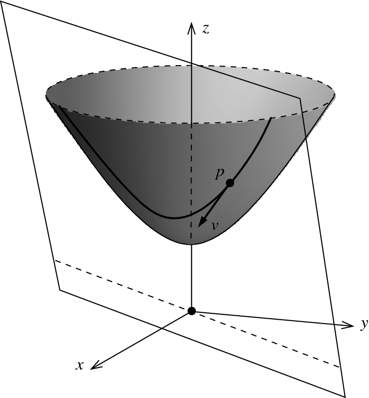
Throughout this section, we let (M, g) be a Riemannian or pseudo-Riemannian n-manifold, endowed with its Levi-Civita connection. Corollary 4.28 showed that each initial point $p\in M$ and each initial velocity vector $v\in T_pM$ determine a unique maximal geodesic $\gamma _v$ . To deepen our understanding of geodesics, we need to study their collective behavior, and in particular, to address the following question: How do geodesics change if we vary the initial point or the initial velocity? The dependence of geodesics on the initial data is encoded in a map from the tangent bundle into the manifold, called the exponential map, whose properties are fundamental to the further study of Riemannian geometry.

(It is worth noting that the existence of the exponential map and the basic properties expressed in Proposition 5.19 below hold for every connection in TM, not just for the Levi-Civita connection. For simplicity, we restrict attention here to the latter case, because that is all we need. We also restrict to manifolds without boundary, in order to avoid complications with geodesics running into a boundary.)

The next lemma shows that geodesics with proportional initial velocities are related in a simple way.

Lemma 5.18

(Rescaling Lemma). For every $p\in M$ , $v\in T_pM$ , and $c, t\in \mathbb {R}$ ,

$\begin{aligned} \gamma _{cv}(t) = \gamma _v(ct), \end{aligned}$

(5.16)

whenever either side is defined.

Proof.

If $$c=0$$ , then both sides of (5.16) are equal to p for all $t\in \mathbb {R}$ , so we may assume that $c\ne 0$ . It suffices to show that $\gamma _{cv}(t)$ exists and (5.16) holds whenever the right-hand side is defined. (The same argument with the substitutions $$v= c'v'$$ , $$t=c't'$$ , and $$c=1/c'$$ then implies that the conclusion holds when only the left-hand side is known to be defined.)

Suppose the maximal domain of $\gamma _v$ is the open interval $I\subseteq \mathbb {R}$ . For simplicity, write $\gamma =\gamma _v$ , and define a new curve $\tilde{\gamma }:c^{-1}I\mathrel {\rightarrow }M$ by $\tilde{\gamma }(t) = \gamma (ct)$ , where $c^{-1}I =\{c^{-1}t:t\in I\}$ . We will show that $\tilde{\gamma }$ is a geodesic with initial point p and initial velocity cv; it then follows by uniqueness and maximality that it must be equal to $\gamma _{cv}$ .

It is immediate from the definition that $\tilde{\gamma }(0)=\gamma (0)=p$ . Choose any smooth local coordinates on M and write the coordinate representation of $\gamma$ as $\gamma (t)=\big (\gamma ^1(t),\dots ,\gamma ^n(t)\big )$ ; then the chain rule gives

$\begin{aligned} \begin{aligned} \dot{\tilde{\gamma }}{}^i(t)&= \frac{d}{dt}\gamma ^i(ct)\\&= c\dot{\gamma }^i(ct). \end{aligned} \end{aligned}$

In particular, it follows that ${\tilde{\gamma }'}(0) = c\gamma '(0)=cv$ .

Now let

and $\tilde{D}_t$ denote the covariant differentiation operators along $\gamma$ and $\tilde{\gamma }$ , respectively. Using the chain rule again in coordinates yields

$\begin{aligned} \begin{aligned} {\tilde{D}_t {\tilde{\gamma }'}}(t)&= \left( \frac{d}{dt} \dot{\tilde{\gamma }}{}^k(t) + \Gamma ^k_{ij}\big (\tilde{\gamma }(t)\big ) \dot{\tilde{\gamma }}{}^i(t) \dot{\tilde{\gamma }}{}^j(t)\right) \partial _{k}\\&= \left( c^2\ddot{\gamma }{}^k(ct) + c^2\Gamma ^k_{ij}(\gamma (ct)) \dot{\gamma }^i(ct) \dot{\gamma }^j(ct)\right) \partial _{k}\\&= c^2{D_t\gamma '}(ct) = 0. \end{aligned} \end{aligned}$

Thus $\tilde{\gamma }$ is a geodesic, so $\tilde{\gamma }= \gamma _{cv}$ , as claimed. $\square$

The assignment $v\mapsto \gamma _v$ defines a map from TM to the set of geodesics in M. More importantly, by virtue of the rescaling lemma, it allows us to define a map from (a subset of) the tangent bundle to M itself, which sends each line through the origin in $$T_pM$$ to a geodesic.

Define a subset $\mathscr {E}\subseteq TM$ , the domain of the exponential map , by

$\begin{aligned} \mathscr {E} = \{ v\in TM: \gamma _v \text { is defined on an interval containing}\,\, [0,1]\}, \end{aligned}$

and then define the exponential map $\exp :\mathscr {E}\mathrel {\rightarrow }M$ by

$\begin{aligned} \exp (v) = \gamma _v(1). \end{aligned}$

For each $p\in M$ , the restricted exponential map at p, denoted by $\exp _p$ , is the restriction of $\exp$ to the set $\mathscr {E}_p = \mathscr {E}\mathbin {\cap }T_pM$ .

The exponential map of a Riemannian manifold should not be confused with the exponential map of a Lie group. The two are closely related for bi-invariant metrics (see Problem 5-8), but in general they need not be. To avoid confusion, we always designate the exponential map of a Lie group G by $\exp ^G$ , and reserve the undecorated notation $\exp$ for the Riemannian exponential map.

The next proposition describes some essential features of the exponential map. Recall that a subset of a vector space V is said to be star-shaped with respect to a point $x\in S$ if for every $y\in S$ , the line segment from x to y is contained in S.

Proposition 5.19

(Properties of the Exponential Map). Let (M, g) be a Riemannian or pseudo-Riemannian manifold, and let $\exp :\mathscr {E}\mathrel {\rightarrow }M$ be its exponential map.

(a)
$\mathscr {E}$ is an open subset of TM containing the image of the zero section, and each set $\mathscr {E}_p\subseteq T_pM$ is star-shaped with respect to 0.
(b)
For each $v\in TM$ , the geodesic $\gamma _v$ is given by
$\begin{aligned} \gamma _v(t) = \exp (tv) \end{aligned}$

(5.17)
for all t such that either side is defined.
(c)
The exponential map is smooth.
(d)
Foreach point $p\in M$ , the differential $d\left( \exp _p\right) _0:T_0(T_pM)\cong T_pM\mathrel {\rightarrow }T_pM$ is the identity map of , under the usual identification of with .

Proof.

Write $n=\dim M$ . The rescaling lemma with $$t=1$$

says precisely that $\exp (cv) = \gamma _{cv}(1) =\gamma _{v}(c)$ whenever either side is defined; this is (b). Moreover, if $v\in \mathscr {E}_p$ , then by definition $\gamma _v$ is defined at least on [0, 1]. Thus for $0\le t\le 1$ , the rescaling lemma says that

$\begin{aligned} \exp _p(tv) = \gamma _{tv}(1) = \gamma _v(t) \end{aligned}$

is defined. This shows that $\mathscr {E}_p$ is star-shaped with respect to 0.

Next we will show that $\mathscr {E}$ is open and $\exp$ is smooth. To do so, we revisit the proof of the existence and uniqueness theorem for geodesics (Theorem 4.27) and reformulate it in a more invariant way. Let $\big (x^i\big )$ be any smooth local coordinates on an open set $U\subseteq M$ , let $\pi :TM\mathrel {\rightarrow }M$ be the projection, and let $\big (x^i, v^i\big )$ denote the associated natural coordinates for $\pi ^{-1}(U)\subseteq TM$ (see p. 384). In terms of these coordinates, formula (4.18) defines a smooth vector field G on $\pi ^{-1}(U)$ . The integral curves of G are the curves $\eta (t) = \big (x^1(t),\dots ,x^n(t), v^1(t),\dots , v^n(t)\big )$ that satisfy the system of ODEs given by (4.17), which is equivalent to the geodesic equation under the substitution $v^k=\dot{x}^k$ , as we observed in the proof of Theorem 4.27. Stated somewhat more invariantly, every integral curve of G on $\pi ^{-1}(U)$ projects to a geodesic under $\pi :TM\mathrel {\rightarrow }M$ (which in these coordinates is just $\pi (x, v)=x$ ); conversely, every geodesic $\gamma (t)=\big (x^1(t),\dots , x^n(t)\big )$ in U lifts to an integral curve of G in $\pi ^{-1}(U)$ by setting $v^i(t) = \dot{x}^i(t)$ .

The importance of G stems from the fact that it actually defines a global vector field on the total space of TM, called the geodesic vector field. We could verify this by computing the transformation law for the components of G under a change of coordinates and showing that they take the same form in every coordinate chart; but fortunately there is a way to avoid that messy computation. The key observation, to be proved below, is that G acts on a function $f\in C^\infty (TM)$ by

$\begin{aligned} Gf(p, v) = \left. \frac{d}{dt} \right| _{t=0} f\big (\gamma _v(t),\gamma _v'(t)\big ). \end{aligned}$

(5.18)

(Here and whenever convenient, we use the notations (p, v) and v interchangeably for an element $v\in T_pM$ , depending on whether we wish to emphasize the point at which v is tangent.) Since this formula is independent of coordinates, it shows that the various definitions of G given by (4.18) in different coordinate systems agree.

To prove that G satisfies (5.18), we write the components of the geodesic $\gamma _v(t)$ as $$x^i(t)$$

and those of its velocity as $v^i(t)=\dot{x}^i(t)$ . Using the chain rule and the geodesic equation in the form (4.17), we can write the right-hand side of (5.18) as

$\begin{aligned} \begin{aligned} \left( \frac{\partial f}{\partial x^k}(x(t),v(t)) \dot{x}^k(t)\right.&+ \left. \left. \frac{\partial f}{\partial v^k}(x(t), v(t)) \dot{v}^k(t)\right) \right| _{t=0}\\&= \frac{\partial f}{\partial x^k}(p,v) v^k - \frac{\partial f}{\partial v^k}(p,v) v^iv^j\Gamma ^k_{ij}(p)\\&= Gf(p, v). \end{aligned} \end{aligned}$

The fundamental theorem on flows (Thm. A.42) shows that there exist an open set $\mathscr {D}\subseteq \mathbb {R}\times TM$ containing $\{0\}\times TM$ and a smooth map $\theta :\mathscr {D}\mathrel {\rightarrow }TM$ , such that each curve $\theta ^{(p,v)}(t) = \theta (t,(p, v))$ is the unique maximal integral curve of G starting at (p, v), defined on an open interval containing 0.

Now suppose $(p, v)\in \mathscr {E}$ . This means that the geodesic $\gamma _v$ is defined at least on the interval [0, 1], and therefore so is the integral curve of G starting at $(p, v)\in ~TM$ . Since $(1,(p, v))\in \mathscr {D}$ , there is a neighborhood of (1, (p, v)) in $\mathbb {R}\times TM$ on which the flow of G is defined (Fig. 5.2). In particular, this means that there is a neighborhood of (p, v) on which the flow exists for $t\in [0,1]$ , and therefore on which the exponential map is defined. This shows that $\mathscr {E}$ is open.

Since geodesics are projections of integral curves of G, it follows that the exponential map can be expressed as

$\begin{aligned} \exp _p(v) = \gamma _v(1) = \pi \circ \theta (1,(p, v)) \end{aligned}$

wherever it is defined, and therefore $\exp _p(v)$ is a smooth function of (p, v).

To compute $d\big (\exp _p\big )_0 (v)$ for an arbitrary vector $v\in T_pM$ , we just need to choose a curve $\tau$ in $$T_pM$$

starting at 0 whose initial velocity is v, and compute the initial velocity of $\exp _p\circ \tau$ . A convenient curve is $\tau (t)=tv$ , which yields

$\begin{aligned} d\big (\exp _p\big )_0(v)= \left. \frac{d}{dt}\right| _{t=0} (\exp _p\circ \tau )(t)=\left. \frac{d}{dt}\right| _{t=0} \exp _p(tv)=\left. \frac{d}{dt}\right| _{t=0} \gamma _v(t)= v. \end{aligned}$

Thus $d\big (\exp _p\big )_0$ is the identity map. $\square$

../images/56724_2_En_5_Chapter/56724_2_En_5_Fig2_HTML.png — Fig. 5.2:
$\mathscr {E}$ is open

$$\mathscr {E}$$ — Fig. 5.2:
$\mathscr {E}$ is open

Corollary 5.14 on the naturality of geodesics translates into the following important property of the exponential map.

Proposition 5.20

(Naturality of the Exponential Map). Suppose (M, g) and $\big ({{\widetilde{M}}},\tilde{g}\big )$ are Riemannian or pseudo-Riemannian manifolds and $\varphi :M\mathrel {\rightarrow }{{\widetilde{M}}}$ is a local isometry. Then for every $p\in M$ , the following diagram commutes:

../images/56724_2_En_5_Chapter/56724_2_En_5_Equ87_HTML.png

where $\mathscr {E}_p\subseteq T_pM$ and $\tilde{\mathscr {E}}_{\varphi (p)}\subseteq T_{\varphi (p)}{{\widetilde{M}}}$ are the domains of the restricted exponential maps $\exp _p$ (with respect to g) and $\exp _{\varphi (p)}$ (with respect to $\tilde{g}$ ), respectively.

$\blacktriangleright$ Exercise 5.21. Prove Proposition 5.20.

An important consequence of the naturality of the exponential map is the following proposition, which says that local isometries of connected manifolds are completely determined by their values and differentials at a single point.

Proposition 5.22.

Let (M, g) and $\big ({{\widetilde{M}}},\tilde{g}\big )$ be Riemannian or pseudo-Riemannian manifolds, with M connected. Suppose $\varphi , \psi :M\mathrel {\rightarrow }{{\widetilde{M}}}$ are local isometries such that for some point $p\in M$ , we have $\varphi (p)=\psi (p)$ and $d\varphi _p=d\psi _p$ . Then $\varphi \equiv \psi$ .

Proof.

Problem 5-10. $\square$

A Riemannian or pseudo-Riemannian manifold (M, g) is said to be geodesically complete if every maximal geodesic is defined for all $t\in \mathbb {R}$ , or equivalently if the domain of the exponential map is all of TM. It is easy to construct examples of manifolds that are not geodesically complete; for example, in every proper open subset of $\mathbb {R}^n$ with its Euclidean metric or with a pseudo-Euclidean metric, there are geodesics that reach the boundary in finite time. Similarly, on $\mathbb {R}^n$ with the metric $(\sigma ^{-1})^*\mathring{g}$ obtained from the sphere by stereographic projection, there are geodesics that escape to infinity in finite time. Geodesically complete manifolds are the natural setting for global questions in Riemannian or pseudo-Riemannian geometry; beginning with Chapter 6, most of our attention will be focused on them.

Normal Neighborhoods and Normal Coordinates

We continue to let (M, g) be a Riemannian or pseudo-Riemannian manifold of dimension n (without boundary). Recall that for every $p\in M$ , the restricted exponential map $\exp _p$ maps the open subset $\mathscr {E}_p\subseteq T_pM$ smoothly into M. Because $d\big (\exp _p\big )_0$ is invertible, the inverse function theorem guarantees that there exist a neighborhood V of the origin in $$T_pM$$ and a neighborhood U of p in M such that $\exp _p:V\mathrel {\rightarrow }U$ is a diffeomorphism. A neighborhood U of $p\in M$ that is the diffeomorphic image under $\exp _p$ of a star-shaped neighborhood of $0\in T_pM$ is called a normal neighborhood of ${\varvec{p}}$ .

Every orthonormal basis $$(b_i)$$

for

determines a basis isomorphism $B:\mathbb {R}^n\mathrel {\rightarrow }T_pM$ by $B(x^1,\dots , x^n) = x^ib_i$ . If $U=\exp _p(V)$ is a normal neighborhood of p, we can combine this isomorphism with the exponential map to get a smooth coordinate map $\varphi =B^{-1}\circ (\exp _p|_V)^{-1}:U\mathrel {\rightarrow }\mathbb {R}^n$ :

../images/56724_2_En_5_Chapter/56724_2_En_5_Equ88_HTML.png

Such coordinates are called (Riemannian or pseudo-Riemannian) normal coordinates centered at ${\varvec{p}}$ .

Proposition 5.23

(Uniqueness of Normal Coordinates). Let (M, g) be a Riemannian or pseudo-Riemannian n-manifold, p a point of M, and U a normal neighborhood of p. For every normal coordinate chart on U centered at p, the coordinate basis is orthonormal at p; and for every orthonormal basis $$(b_i)$$

for

, there is a unique normal coordinate chart $\big (x^i\big )$ on U such that $\partial _i|_p = b_i$ for $i=1,\dots , n$ . In the Riemannian case, any two normal coordinate charts $\big (x^i\big )$ and $\big (\tilde{x}^j\big )$ are related by

$\begin{aligned} \tilde{x}^j = A^j_i x^i \end{aligned}$

(5.19)

for some (constant) matrix $\big (A^j_i\big )\in {{\,\mathrm{O}\,}}(n)$ .

Proof.

Let $\varphi$ be a normal coordinate chart on U centered at p, with coordinate functions $\big (x^i\big )$ . By definition, this means that $\varphi = B^{-1}\circ \exp _p^{-1}$ , where $B:\mathbb {R}^n\mathrel {\rightarrow }T_pM$ is the basis isomorphism determined by some orthonormal basis $$(b_i)$$ for $$T_pM$$ . Note that $d\varphi _p^{-1} =d\big (\exp _p\big )_0 \circ dB_0 = B$ because $d\big (\exp _p\big )_0$ is the identity and B is linear. Thus $\partial _i|_p = d\varphi _p^{-1} (\partial _i|_0) = B(\partial _i|_0) = b_i$ , which shows that the coordinate basis is orthonormal at p. Conversely, every orthonormal basis $$(b_i)$$ for $$T_pM$$ yields a basis isomorphism B and thus a normal coordinate chart $\varphi = B^{-1}\circ \exp _p^{-1}$ , which satisfies $\partial _i|_p = b_i$ by the computation above.

If $\tilde{\varphi }= \tilde{B}^{-1}\circ \exp _p^{-1}$ is another such chart, then

$\begin{aligned} \tilde{\varphi }\circ \varphi ^{-1} = \tilde{B}^{-1}\circ \exp _p^{-1}\circ \exp _p \circ B = \tilde{B}^{-1}\circ B, \end{aligned}$

which is a linear isometry of $\mathbb {R}^n$ and therefore has the form (5.19) in terms of standard coordinates on $\mathbb {R}^n$ . Since $\big (\tilde{x}^j\big )$ and $\big (x^i\big )$ are the same coordinates if and only if $\big (A^j_i\big )$ is the identity matrix, this shows that the normal coordinate chart associated with a given orthonormal basis is unique. $\square$

Proposition 5.24

(Properties of Normal Coordinates). Let (M, g) be a Riemannian or pseudo-Riemannian n-manifold, and let $\bigl (U,\bigl (x^i\bigr )\bigr )$ be any normal coordinate chart centered at $p\in M$ .

(a)
The coordinates of p are $(0,\dots , 0)$ .
(b)
The components of the metric at p are $g_{ij} = \delta _{ij}$ if g is Riemannian, and $g_{ij} = \pm \delta _{ij}$ otherwise.
(c)
For every $v=v^i\partial _i|_p\in T_pM$ , the geodesic $\gamma _v$ starting at p with initial velocity v is represented in normal coordinates by the line
$\begin{aligned} \gamma _v(t) = \big (tv^1,\dots , tv^n\big ), \end{aligned}$

(5.20)
as long as t is in some interval I containing 0 such that $\gamma _v(I)\subseteq U$ .
(d)
The Christoffel symbols in these coordinates vanish at p.
(e)
All of the first partial derivatives of $g_{ij}$ in these coordinates vanish at p.

Proof.

Part (a) follows directly from the definition of normal coordinates, and parts (b) and (c) follow from Propositions 5.23 and 5.19(b), respectively.

To prove (d), let $v=v^i\partial _i|_p\in T_pM$ be arbitrary. The geodesic equation (4.16) for $\gamma _v(t) = \big (tv^1,\dots , tv^n\big )$ simplifies to

$\begin{aligned} \Gamma _{ij}^k(tv) v^i v^j=0. \end{aligned}$

Evaluating this expression at $$t=0$$

shows that $\smash {\Gamma _{ij}^k(0)v^iv^j=0}$ for every index k and every vector v. In particular, with $v=\partial _a$ for some fixed a, this shows that $\Gamma _{aa}^k=0$ for each a and k (no summation). Substituting $v={\partial _a + \partial _b}$ and $v={\partial _b - \partial _a}$ for any fixed pair of indices a and b and subtracting, we conclude also that $\smash {\Gamma _{ab}^k}= 0$ at p for all a, b, k. Finally, (e) follows from (d) together with (5.2) in the case $E_k = \partial _k$ . $\square$

Because they are given by the simple formula (5.20), the geodesics starting at p and lying in a normal neighborhood of p are called radial geodesics . (But be warned that geodesics that do not pass through p do not in general have a simple form in normal coordinates.)

Tubular Neighborhoods and Fermi Coordinates

The exponential map and normal coordinates give us a good understanding of the behavior of geodesics starting a point. In this section, we generalize those constructions to geodesics starting on any embedded submanifold. We restrict attention to the Riemannian case, because we will be using the Riemannian distance function.

Suppose (M, g) is a Riemannian manifold, $P\subseteq M$ is an embedded submanifold, and $\pi :NP\mathrel {\rightarrow }P$ is the normal bundle of P in M. Let $\mathscr {E}\subseteq TM$ denote the domain of the exponential map of M, and let $\mathscr {E}_P = \mathscr {E}\cap NP$ . Let $E:\mathscr {E}_P\mathrel {\rightarrow }M$ denote the restriction of $\exp$ (the exponential map of M) to $\mathscr {E}_P$ . We call E the normal exponential map of P in M .

A normal neighborhood of P in M is an open subset $U\subseteq M$ that is the diffeomorphic image under E of an open subset $V\subseteq \mathscr {E}_P$ whose intersection with each fiber $$N_xP$$

is star-shaped with respect to 0. We will be primarily interested in normal neighborhoods of the following type: a normal neighborhood of P in M is called a tubular neighborhood if it is the diffeomorphic image under E of a subset $V\subseteq \mathscr {E}_P$ of the form

$\begin{aligned} V = \big \{ (x, v)\in NP: |v|_g < \delta (x)\big \}, \end{aligned}$

(5.21)

for some positive continuous function $\delta :P\mathrel {\rightarrow }\mathbb {R}$ (Fig. 5.3). If U is the diffeomorphic image of such a set V for a constant function $\delta (x)\equiv \varepsilon$ , then it is called a uniform tubular neighborhood of radius $\varepsilon$ , or an ${\varvec{\varepsilon }}$ -tubular neighborhood.

../images/56724_2_En_5_Chapter/56724_2_En_5_Fig3_HTML.png — Fig. 5.3:
A tubular neighborhood

../images/56724_2_En_5_Chapter/56724_2_En_5_Fig4_HTML.png — Fig. 5.4:
Injectivity of E

Theorem 5.25

(Tubular Neighborhood Theorem). Let (M, g) be a Riemannian manifold. Every embedded submanifold of M has a tubular neighborhood in M, and every compact submanifold has a uniform tubular neighborhood.

Proof.

Let $P\subseteq M$ be an embedded submanifold, and let $P_0\subseteq NP$ be the subset $\{(x, 0):x\in P\}$ (the image of the zero section of NP). We begin by showing that the normal exponential map E is a local diffeomorphism on a neighborhood of $$P_0$$

. By the inverse function theorem, it suffices to show that the differential $dE_{(x, 0)}$ is bijective at each point $(x, 0)\in P_0$ . The restriction of E to $$P_0$$

is just the diffeomorphism $P_0\mathrel {\rightarrow }P$ followed by the embedding $P\mathrel {\hookrightarrow }M$ , so $dE_{(x, 0)}$ maps the subspace $T_{(x, 0)}P_0\subseteq T_{(x, 0)}NP$ isomorphically onto $$T_xP$$

. On the other hand, on the fiber $$N_xP$$

, E agrees with the restricted exponential map $\exp _x$ , which is a diffeomorphism near 0, so $dE_{(x, 0)}$ maps $T_{(x, 0)}(N_xP)\subseteq T_{(x, 0)}NP$ isomorphically onto $$N_xP$$

. Since $T_x M=T_xP\oplus N_xP$ , this shows that $dE_{(x, 0)}$ is surjective, and hence it is bijective for dimensional reasons. Thus E is a diffeomorphism on a neighborhood of (x, 0) in NP, which we can take to be of the form

$\begin{aligned} V_\delta (x) = \left\{ (x',v')\in NP: d_g(x, x')<\delta ,\ |v'|_g<\delta \right\} \end{aligned}$

(5.22)

for some $\delta >0$ . (Here we are using the fact that P is embedded in M, so it has the subspace topology.)

To complete the proof, we need to show that there is a set $V\subseteq \mathscr {E}_P$ of the form (5.21) on which E is a diffeomorphism onto its image. For each point $x\in P$ , define

$\begin{aligned} \varDelta (x) = \sup \big \{ \delta \le 1: E~\text {is a diffeomorphism from}~V_\delta (x) \text { to its image}\big \}. \end{aligned}$

(5.23)

The argument in the preceding paragraph implies that $\varDelta (x)$ is positive for each x. Note that E is injective on the entire set $V_{\varDelta (x)}(x)$ , because any two points $$(x_1,v_1),(x_2,v_2)$$

in this set are in $V_\delta (x)$ for some $\delta <\varDelta (x)$ . Because it is an injective local diffeomorphism, E is actually a diffeomorphism from $V_{\varDelta (x)}(x)$ onto its image.

Next we show that the function $\varDelta :P\mathrel {\rightarrow }\mathbb {R}$ is continuous. For any $x, x'\in P$ , if $d_g(x, x')<\varDelta (x)$ , then the triangle inequality shows that $V_{\delta }(x')$ is contained in $V_{\varDelta (x)}(x)$ for $\delta =\varDelta (x)-d_g(x, x')$ , which implies that $\varDelta (x')\ge \varDelta (x)-d_g(x, x')$ , or

$\begin{aligned} \varDelta (x)-\varDelta (x') \le d_g(x, x'). \end{aligned}$

(5.24)

If $d_g(x, x')\ge \varDelta (x)$ , then (5.24) holds for trivial reasons. Reversing the roles of x and $$x'$$

yields an analogous inequality, which shows that $|\varDelta (x)-\varDelta (x')| \le d_g(x, x')$ , so $\varDelta$ is continuous.

Let $V = \bigl \{(x, v)\in NP: |v|_g<\tfrac{1}{2}\varDelta (x)\bigr \}$ , which is an open subset of NP containing $$P_0$$

. We show that E is injective on V. Suppose (x, v) and $$(x', v')$$

are points in V such that $$E(x,v) = E(x', v')$$

(Fig. 5.4). Assume without loss of generality that $\varDelta (x')\le \varDelta (x)$ . Because $\exp _x(v) = \exp _{x'}(v')$ , there is an admissible curve from x to $$x'$$

of length

, and thus

$\begin{aligned} d_g(x, x') \le |v|_g+|v'|_g < \tfrac{1}{2}\varDelta (x) + \tfrac{1}{2}\varDelta (x')\le \varDelta (x). \end{aligned}$

Therefore, both (x, v) and $$(x', v')$$

are in $V_{\varDelta (x)}(x)$ . Since E is injective on this set, this implies $$(x,v) =(x', v')$$

The set $$U= E(V)$$ is open in M because $$E|_V$$ is a local diffeomorphism and thus an open map, and $E:V\mathrel {\rightarrow }U$ is a diffeomorphism. Therefore, U is a tubular neighborhood of P.

Finally, if P is compact, then the continuous function $\tfrac{1}{2}\varDelta$ achieves a minimum value $\varepsilon >0$ on P, so U contains a uniform tubular neighborhood of radius $\varepsilon$ . $\square$

Fermi Coordinates

Now we will construct coordinates on a tubular neighborhood that are analogous to Riemannian normal coordinates around a point. Let P be an embedded p-dimensional submanifold of a Riemannian n-manifold (M, g), and let $U\subseteq M$ be a normal neighborhood of P, with $$U=E(V)$$ for some appropriate open subset $V\subseteq NP$ .

Let $(W_0,\psi )$ be a smooth coordinate chart for P, and let $(E_1,\dots , E_{n-p})$ be a local orthonormal frame for the normal bundle NP; by shrinking $$W_0$$

if necessary, we can assume that the coordinates and the local frame are defined on the same open subset $W_0\subseteq P$ . Let ${{\widehat{W}}}_0 = \psi (W_0)\subseteq \mathbb {R}^p$ , and let $NP|_{W_0}$ be the portion of the normal bundle over $$W_0$$

. The coordinate map $\psi$ and frame $$(E_j)$$

yield a diffeomorphism $B:{{\widehat{W}}}_0\times \mathbb {R}^{n-p} \mathrel {\rightarrow }NP|_{W_0}$ defined by

$\begin{aligned} B\big (x^1,\dots ,x^p, v^1,\dots , v^{n-p}\big ) = \big ( q, \ v^1 E_1|_q+ \dots + v^{n-p} E_{n-p}|_q\big ), \end{aligned}$

where $q=\psi ^{-1}(x^1,\dots , x^p)$ . Let $V_0=V\cap NP|_{W_0}\subseteq NP$ and $U_0= E(V_0)\subseteq M$ , and define a smooth coordinate map $\varphi :U_0\mathrel {\rightarrow }\mathbb {R}^n$ by $\varphi = B^{-1} \circ \big (E|_{V_0}\big )^{-1}$ :

../images/56724_2_En_5_Chapter/56724_2_En_5_Equ89_HTML.png

The coordinate map can also be written

$\begin{aligned} \varphi :E\big (q, v^1 E_1|_q + \dots + v^{n-p} E_{n-p}|_q\big ) \mapsto \big ( x^1(q),\dots ,x^p(q), v^1,\dots , v^{n-p}\big ). \end{aligned}$

(5.25)

Coordinates of this form are called Fermi coordinates , after the Italian physicist Enrico Fermi (1901–1954), who first introduced them in the special case in which P is the image of a geodesic in M. The generalization to arbitrary submanifolds was first introduced by Alfred Gray [Gra82]. (See also [Gra04] for a detailed study of the geometry of tubular neighborhoods.)

Here is the analogue of Proposition 5.24 for Fermi coordinates.

Proposition 5.26

(Properties of Fermi Coordinates). Let P be an embedded p-dimensional submanifold of a Riemannian n-manifold (M, g), let U be a normal neighborhood of P in M, and let $\big (x^1,\dots ,x^p, v^1,\dots , v^{n-p}\big )$ be Fermi coordinates on an open subset $U_0\subseteq U$ . For convenience, we also write $x^{p+j} = v^{j}$ for $j=1,\dots , n-p$ .

(a)
$P\cap U_0$ is the set of points where $x^{p+1}=\dots =x^n=0$ .
(b)
At each point $q\in P\cap U_0$ , the metric components satisfy the following:
$\begin{aligned} g_{ij} = g_{ji} = {\left\{ \begin{array}{ll} 0, &{} 1\le i\le p\ \text { and }\ p+1\le j \le n,\\ \delta _{ij}, &{}p+1\le i, j\le n. \end{array}\right. } \end{aligned}$
(c)
For every $q\in P\cap U_0$ and $v = v^1E_1|_q + \dots + v^{n-p}E_{n-p}|_q\in N_q P$ , the geodesic $\gamma _v$ starting at q with initial velocity v is the curve with coordinate expression $\gamma _v(t) = \big (x^1(q),\dots ,x^p(q), tv^1,\dots , tv^{n-p}\big )$ .
(d)
At each $q\in P\cap U_0$ , the Christoffel symbols in these coordinates satisfy $\Gamma _{ij}^k {=} 0$ , provided $p+1\le i, j\le n$ .
(e)
At each $q \in P\cap U_0$ , the partial derivatives $\partial _i g_{jk}(q)$ vanish for $p+1\le i,j, k \le n$ .

Proof.

Problem 5-18. $\square$

Geodesics of the Model Spaces

In this section we determine the geodesics of the three types of frame-homogeneous Riemannian manifolds defined in Chapter 3. We could, of course, compute the Christoffel symbols of these metrics in suitable coordinates, and try to find the geodesics by solving the appropriate differential equations; but for these spaces, much easier methods are available based on symmetry and other geometric considerations.

Euclidean Space

On $\mathbb {R}^n$ with the Euclidean metric, Proposition 5.12 shows that the Levi-Civita connection is the Euclidean connection. Therefore, as one would expect, constant-coefficient vector fields are parallel, and the Euclidean geodesics are straight lines with constant-speed parametrizations (Exercises 4.29 and 4.30). Every Euclidean space is geodesically complete.

Spheres

Because the round metric on the sphere $\mathbb S^n(R)$ is induced by the Euclidean metric on $\mathbb {R}^{n+1}$ , it is easy to determine the geodesics on a sphere using Corollary 5.2. Define a great circle on $\mathbb S^n(R)$ to be any subset of the form $\mathbb S^n(R)\cap \varPi$ , where $\varPi \subseteq \mathbb {R}^{n+1}$ is a 2-dimensional linear subspace.

Proposition 5.27.

A nonconstant curve on $\mathbb S^n(R)$ is a maximal geodesic if and only if it is a periodic constant-speed curve whose image is a great circle. Thus every sphere is geodesically complete.

Proof.

Let $p\in \mathbb S^n(R)$ be arbitrary. Because $$f(x) = |x|^2$$ is a defining function for $\mathbb S^n(R)$ , a vector $v\in T_p\mathbb {R}^{n+1}$ is tangent to $\mathbb S^n(R)$ if and only if $df_p(v) = 2\langle v, p \rangle =0$ , where we think of p as a vector by means of the usual identification of $\mathbb {R}^{n+1}$ with $T_p\mathbb {R}^{n+1}$ . Thus $T_p\mathbb S^n(R)$ is exactly the set of vectors orthogonal to p.

Suppose v is an arbitrary nonzero vector in $T_p \mathbb S^n(R)$ . Let $$a = |v|/R$$

and $\hat{v} = v/a$ (so $|\hat{v}| = R$ ), and consider the smooth curve $\gamma :\mathbb {R}\mathrel {\rightarrow }\mathbb {R}^{n+1}$ given by

$\begin{aligned} \gamma (t) = (\cos a t) p + (\sin a t) \hat{v}. \end{aligned}$

By direct computation, $|\gamma (t)|^2 = R^2$ , so $\gamma (t)\in \mathbb S^n(R)$ for all t. Moreover,

$\begin{aligned} \gamma '(t)&= - a (\sin a t) p + a (\cos a t) \hat{v},\\ \gamma ''(t)&= - a^2 (\cos a t) p - a^2 (\sin a t) \hat{v}. \end{aligned}$

Because $\gamma ''(t)$ is proportional to $\gamma (t)$ (thinking of both as vectors in $\mathbb {R}^{n+1}$ ), it follows that $\gamma ''(t)$ is ${\bar{g}}$ -orthogonal to $T_{\gamma (t)}\mathbb S^n(R)$ , so $\gamma$ is a geodesic in $\mathbb S^n(R)$ by Corollary 5.2. Since $\gamma (0)=p$ and $\gamma '(0)= a \hat{v} = v$ , it follows that $\gamma = \gamma _v$ .

Each $\gamma _v$ is periodic of period $2\pi /a$ , and has constant speed by Corollary 5.6 (or by direct computation). The image of $\gamma _v$ is the great circle formed by the intersection of $\mathbb S^n(R)$ with the linear subspace spanned by $\{p,\hat{v}\}$ , as you can check.

Conversely, suppose C is a great circle formed by intersecting $\mathbb S^n(R)$ with a 2-dimensional subspace $\varPi$ , and let $\{v, w\}$ be an orthonormal basis for $\varPi$ . Then C is the image of the geodesic with initial point $$p = Rw$$ and initial velocity v. $\square$

Hyperbolic Spaces

The geodesics of hyperbolic spaces can be determined by an analogous procedure using the hyperboloid model.

../images/56724_2_En_5_Chapter/56724_2_En_5_Fig5_HTML.png — Fig. 5.5:
A great hyperbola

../images/56724_2_En_5_Chapter/56724_2_En_5_Fig6_HTML.png — Fig. 5.6:
Geodesics of $\mathbb {K}^n(R)$

$$\mathbb {K}^n(R)$$ — Fig. 5.6:
Geodesics of $\mathbb {K}^n(R)$

../images/56724_2_En_5_Chapter/56724_2_En_5_Fig7_HTML.png — Fig. 5.7:
Geodesics of $\mathbb B^n(R)$

$$\mathbb B^n(R)$$ — Fig. 5.7:
Geodesics of $\mathbb B^n(R)$

Proposition 5.28.

A nonconstant curve in a hyperbolic space is a maximal geodesic if and only if it is a constant-speed embedding of $\mathbb {R}$ whose image is one of the following:

(a)
Hyperboloid model: The intersection of $\mathbb H^n(R)$ with a 2-dimensional linear subspace of $\mathbb {R}^{n, 1}$ , called a great hyperbola (Fig. 5.5).
(b)
Beltrami–Klein model: The interior of a line segment whose endpoints both lie on $\partial \mathbb {K}^n(R)$ (Fig. 5.6).
(c)
Ball model: The interior of a diameter of $\mathbb B^n(R)$ , or the intersection of $\mathbb B^n(R)$ with a Euclidean circle that intersects $\partial \mathbb B^n(R)$ orthogonally (Fig. 5.7).
(d)
Half-space model: The intersection of $\mathbb {U}^n(R)$ with one of the following: a line parallel to the y-axis or a Euclidean circle with center on $\partial \mathbb {U}^n(R)$ (Fig. 5.8).

Every hyperbolic space is geodesically complete.

../images/56724_2_En_5_Chapter/56724_2_En_5_Fig8_HTML.png — Fig. 5.8:
Geodesics of $\mathbb {U}^n(R)$

$$\mathbb {U}^n(R)$$ — Fig. 5.8:
Geodesics of $\mathbb {U}^n(R)$

Proof.

We begin with the hyperboloid model, for which the proof is formally quite similar to what we just did for the sphere. Since the Riemannian connection on $\mathbb H^n(R)$ is equal to the tangential connection by Proposition 5.12, it follows from Corollary 5.2 that a smooth curve $\gamma :I\mathrel {\rightarrow }\mathbb H^n(R)$ is a geodesic if and only if its acceleration $\gamma ''(t)$ is everywhere $\bar{q}$ -orthogonal to $T_{\gamma (t)}\mathbb H^n(R)$ (where $\bar{q} = \bar{q}^{(n, 1)}$ is the Minkowski metric).

Let $p\in \mathbb H^n(R)$ be arbitrary. Note that $f(x) = \bar{q}(x, x)$ is a defining function for $\mathbb H^n(R)$ , and (3.10) shows that the gradient of f at p is equal to 2p (where we regard p as a vector in $T_p\mathbb {R}^{n, 1}$ as before). It follows that a vector $v\in T_p\mathbb {R}^{n, 1}$ is tangent to $\mathbb H^n(R)$ if and only if $\bar{q}(p, v) =0$ . Let $v\in T_p \mathbb H^n(R)$ be an arbitrary nonzero vector. Put $a = |v|_{\bar{q}}/R = \bar{q}(v, v)^{1/2}/R$ and $\hat{v} = v/a$ , and define $\gamma :\mathbb {R}\mathrel {\rightarrow }\mathbb {R}^{n, 1}$ by

$\begin{aligned} \gamma (t) = (\cosh a t) p + (\sinh a t) \hat{v}. \end{aligned}$

Direct computation shows that $\gamma$ takes its values in $\mathbb H^n(R)$ and that its acceleration vector is everywhere proportional to $\gamma (t)$ . Thus $\gamma ''(t)$ is $\bar{q}$ -orthogonal to $T_{\gamma (t)}\mathbb H^n(R)$ , so $\gamma$ is a geodesic in $\mathbb H^n(R)$ and therefore has constant speed. Because it satisfies the initial conditions $\gamma (0)=p$ and $\gamma '(0)=v$ , it is equal to $\gamma _v$ . Note that $\gamma _v$ is a smooth embedding of $\mathbb {R}$ into $\mathbb H^n(R)$ whose image is the great hyperbola formed by the intersection between $\mathbb H^n(R)$ and the plane spanned by $\{p,\hat{v}\}$ .

Conversely, suppose $\varPi$ is any 2-dimensional linear subspace of $\mathbb {R}^{n, 1}$ that has nontrivial intersection with $\mathbb H^n(R)$ . Choose $p\in \varPi \cap \mathbb H^n(R)$ , and let v be another nonzero vector in $\varPi$ that is $\bar{q}$ -orthogonal to p, which implies $v\in T_p\mathbb H^n(R)$ . Using the computation above, we see that the image of the geodesic $\gamma _v$ is the great hyperbola formed by the intersection of $\varPi$ with $\mathbb H^n(R)$ .

Before considering the other three models, note that since maximal geodesics in $\mathbb H^n(R)$ are constant-speed embeddings of $\mathbb {R}$ , it follows from naturality that maximal geodesics in each of the other models are also constant-speed embeddings of $\mathbb {R}$ . Thus each model is geodesically complete, and to determine the geodesics in the other models we need only determine their images.

Consider the Beltrami–Klein model. Recall the isometry $c:\mathbb H^n(R)\mathrel {\rightarrow }\mathbb {K}^n(R)$ given by $c(\xi ,\tau ) = R\xi /\tau$ (see (3.11)). The image of a maximal geodesic in $\mathbb H^n(R)$ is a great hyperbola, which is the set of points $(\xi ,\tau )\in \mathbb H^n(R)$ that solve a system of $$n-1$$ independent linear equations. Simple algebra shows that $(\xi ,\tau )$ satisfies a linear equation $\alpha _i\xi ^i+ \beta \tau =0$ if and only if $w = c(\xi ,\tau ) = R\xi /\tau$ satisfies the affine equation $\alpha _i w^i = -\beta R$ . Thus c maps each great hyperbola onto the intersection of $\mathbb {K}^n(R)$ with an affine subspace of $\mathbb {R}^n$ , and since it is the image of a smooth curve, it must be the intersection of $\mathbb {K}^n(R)$ with a straight line.

Next consider the Poincaré ball model. First consider the 2-dimensional case, and recall the inverse hyperbolic stereographic projection $\pi ^{-1}:\mathbb B^2(R)\mathrel {\rightarrow }\mathbb H^{2}(R)$ constructed in Chapter 3:

$\begin{aligned} \pi ^{-1}(u)&= (\xi ,\tau ) = \left( \frac{2R^2 u}{R^2-|u|^2}, R \frac{R^2+|u|^2}{R^2-|u|^2} \right) . \end{aligned}$

In this case, a great hyperbola is the set of points on $\mathbb H^2(R)$ that satisfy a single linear equation $\alpha _i \xi ^i + \beta \tau =0$ . In the special case $\beta =0$ , this hyperbola is mapped by $\pi$ to a straight line segment through the origin, as can easily be seen from the geometric definition of $\pi$ . If $\beta \ne 0$ , we can assume (after multiplying through by a constant if necessary) that $\beta =-1$ , and write the linear equation as ../images/56724_2_En_5_Chapter/56724_2_En_5_IEq695_HTML.gif

../images/56724_2_En_5_Chapter/56724_2_En_5_IEq695_HTML.gif

(where the dot represents the Euclidean dot product between elements of $\mathbb {R}^2$ ). Under $\pi ^{-1}$ , this pulls back to the equation

../images/56724_2_En_5_Chapter/56724_2_En_5_Equ90_HTML.png

on the disk, which simplifies to

../images/56724_2_En_5_Chapter/56724_2_En_5_Equ91_HTML.png

Completing the square, we can write this as

$\begin{aligned} |u-R\alpha |^2=R^2(|\alpha |^2-1). \end{aligned}$

(5.26)

If $|\alpha |^2\le 1$ , this locus is either empty or a point on $\partial \mathbb B^2(R)$ , so it contains no points in $\mathbb B^2(R)$ . Since we are assuming that it is the image of a maximal geodesic, we must therefore have $|\alpha |^2>1$ . In that case, (5.26) is the equation of a circle with center $R\alpha$ and radius $R\sqrt{|\alpha |^2-1}$ . At a point $$u_0$$

where the circle intersects $\partial \mathbb B^2(R)$ , the three points 0, $$u_0$$

, and $R\alpha$ form a triangle with sides $$|u_0|=R$$

, $|R\alpha |$ , and $|u_0-R\alpha |$ (Fig. 5.9), which satisfy the Pythagorean identity by (5.26); therefore the circle meets $\partial \mathbb B^2(R)$ in a right angle.

In the higher-dimensional case, a geodesic on $\mathbb H^n(R)$ is determined by a 2-plane. If the 2-plane contains the point $(0,\dots , 0,R)$ , then the corresponding geodesic on $\mathbb B^n(R)$ is a line through the origin as before. Otherwise, we can use an orthogonal transformation in the $(\xi ^1,\dots ,\xi ^n)$ variables (which preserves $\breve{g}_R$ ) to move this 2-plane so that it lies in the $(\xi ^1,\xi ^{2},\tau )$ subspace, and then we are in the same situation as in the 2-dimensional case.

Finally, consider the upper half-space model. The 2-dimensional case is easiest to analyze using complex notation. Recall the complex formula for the Cayley transform $\kappa :\mathbb {U}^2(R)\mathrel {\rightarrow }\mathbb B^2(R)$ given in Chapter 3:

$\begin{aligned} \kappa (z)=w=iR\frac{z-iR}{z+iR}. \end{aligned}$

Substituting this into equation (5.26) and writing $$w=u+iv$$

and $\alpha =a+ib$ in place of $$u=(u^1,u^2)$$

, $\alpha =(\alpha ^1,\alpha ^2)$ , we get

$\begin{aligned} R^2\frac{|z-iR|^2}{|z+iR|^2} - iR^2\bar{\alpha }\frac{z-iR}{z+iR} + iR^2\alpha \frac{\bar{z}+iR}{\bar{z}-iR} + R^2|\alpha |^2 = R^2 (|\alpha |^2-1). \end{aligned}$

Multiplying through by $(z+iR)(\bar{z}-iR)/2R^2$ and simplifying yields

$\begin{aligned} (1-b)|z|^2 - 2a Rx + (b+1)R^2=0. \end{aligned}$

This is the equation of a circle with center on the x-axis, unless $$b=1$$

, in which case the condition $|\alpha |^2>1$ forces $a\ne 0$ , and then it is a straight line $x=\text {constant}$ . The other class of geodesics on the ball, line segments through the origin, can be handled similarly.

In the higher-dimensional case, suppose first that $\gamma :\mathbb {R}\mathrel {\rightarrow }\mathbb {U}^n(R)$ is a maximal geodesic such that $\gamma (0)$ lies on the y-axis and $\gamma '(0)$ is in the span of $\left\{ \partial /\partial x^1,\partial /\partial y\right\}$ . From the explicit formula (3.15) for $\kappa$ , it follows that $\kappa \circ \gamma (0)$ lies on the v-axis in the ball, and $(\kappa \circ \gamma )'(0)$ is in the span of $\left\{ \partial /\partial u^1,\partial /\partial v\right\}$ . The image of the geodesic $\kappa \circ \gamma$ is either part of a line through the origin or an arc of a circle perpendicular to $\partial \mathbb B^n(R)$ , both of which are contained in the $\left( u^1,v\right)$ -plane. By the argument in the preceding paragraph, it then follows that the image of $\gamma$ is contained in the $\left( x^1,y\right)$ -plane and is either a vertical half-line or a semicircle centered on the $$y=0$$ hyperplane. For the general case, note that translations and orthogonal transformations in the x-variables preserve vertical half-lines and circles centered on the $$y=0$$ hyperplane in $\mathbb {U}^n(R)$ , and they also preserve the metric $\breve{g}^3_R$ . Given an arbitrary maximal geodesic $\gamma :\mathbb {R}\mathrel {\rightarrow }\mathbb {U}^n(R)$ , after applying an x-translation we may assume that $\gamma (0)$ lies on the y-axis, and after an orthogonal transformation in the x variables, we may assume that $\gamma '(0)$ is in the span of $\left\{ \partial /\partial x^1,\partial /\partial y\right\}$ ; then the argument above shows that the image of $\gamma$ is either a vertical half-line or a semicircle centered on the $$y=0$$ hyperplane. $\square$

../images/56724_2_En_5_Chapter/56724_2_En_5_Fig9_HTML.png — Fig. 5.9:
Geodesics are arcs of circles orthogonal to the boundary of $\mathbb H^2(R)$

$$\mathbb H^2(R)$$ — Fig. 5.9:
Geodesics are arcs of circles orthogonal to the boundary of $\mathbb H^2(R)$

Euclidean and Non-Euclidean Geometries

In two dimensions, our model spaces can be interpreted as models of classical Euclidean and non-Euclidean plane geometries.

Euclidean Plane Geometry

Euclid’s axioms for plane and spatial geometry, written around 300 BCE, became a model for axiomatic treatments of geometry, and indeed for all of mathematics. As standards of rigor evolved, mathematicians revised and added to Euclid’s axioms in various ways. One axiom system that meets modern standards of rigor was created by David Hilbert [Hil71]. Here (in somewhat simplified form) are his axioms for plane geometry. (See [Hil71, Gan73, Gre93] for more complete treatments of Hilbert’s axioms, and see [LeeAG] for a different axiomatic approach based on the real number system.)

Hilbert’s Axioms For Euclidean Plane Geometry. The terms point, line, lies on, between, and congruent are primitive terms, and are thus left undefined. We make the following definitions:

Given a line l and a point P, we say that ${\varvec{l}}$ contains ${\varvec{P}}$ if P lies on l.
A set of points is said to be collinear if there is a line that contains them all.
Given two distinct points A, B, the segment $\varvec{{\overline{AB}}}$ is the set consisting of A, B, and all points C such that C is between A and B.
The notation $\varvec{{\overline{AB}}\cong {\overline{A'B'}}}$ means that ${\overline{AB}}$ is congruent to ${\overline{A'B'}}$ .
Given two distinct points A, B, the ray $\varvec{{\scriptscriptstyle \overrightarrow{\normalsize AB}} }$ is the set consisting of A, B, and all points C such that either C is between A and B or B is between A and C.
An interior point of the ray ${\scriptscriptstyle \overrightarrow{\normalsize AB}}$ is a point that lies on ${\scriptscriptstyle \overrightarrow{\normalsize AB}}$ and is not equal to A.
Given three noncollinear points A, O, B, the angle $\varvec{\angle AOB}$ is the union of the rays ${\scriptscriptstyle \overrightarrow{\normalsize OA}}$ and ${\scriptscriptstyle \overrightarrow{\normalsize OB}}$ .
The notation $\varvec{\angle {ABC}\cong \angle {A'B'C'}}$ means that $\angle {ABC}$ is congruent to $\angle {A'B'C'}$ .
Given a line l and two points A, B that do not lie on l, we say that ${\varvec{A}}$ and ${\varvec{B}}$ are on the same side of ${\varvec{l}}$ if no point of ${\overline{AB}}$ lies on l.
Two lines are said to be parallel if there is no point that lies on both of them.

These terms are assumed to satisfy the following postulates, among others:

Incidence Postulates:
1. (a)
  For any two distinct points A, B, there exists a unique line that contains both of them.
2. (b)
  There exist at least two points on each line, and there exist at least three noncollinear points.
Order Postulates:
1. (a)
  If a point B lies between a point A and a point C, then A, B, C are three distinct points of a line, and B also lies between C and A.
2. (b)
  Given two distinct points A and C, there always exists at least one point B such that C lies between A and B.
3. (c)
  Given three distinct points on a line, no more than one of them lies between the other two.
4. (d)
  Let A, B, C be three noncollinear points, and let l be a line that does not contain any of them. If l contains a point of ${\overline{AB}}$ , then it also contains a point of ${\overline{AC}}$ or ${\overline{BC}}$ .
Congruence Postulates:
1. (a)
  If A, B are two points on a line l, and is a point on a line , then it is always possible to find a point on a given ray of starting at such that ${\overline{AB}}\cong {\overline{A'B'}}$ .
2. (b)
  If segments ${\overline{A'B'}}$ and ${\overline{A''B''}}$ are congruent to the same segment ${\overline{AB}}$ , then ${\overline{A'B'}}$ and ${\overline{A''B''}}$ are congruent to each other.
3. (c)
  On a line l, let ${\overline{AB}}$ and ${\overline{BC}}$ be two segments that, except for B, have no points in common. Furthermore, on the same or another line , let ${\overline{A'B'}}$ and ${\overline{B'C'}}$ be two segments that, except for , have no points in common. In that case, if ${\overline{AB}}\cong {\overline{A'B'}}$ and ${\overline{BC}}\cong {\overline{B'C'}}$ , then ${\overline{AC}}\cong {\overline{A'C'}}$ .
4. (d)
  Let $\angle rs$ be an angle and a line, and let a definite side of be given. Let ${\scriptscriptstyle \overrightarrow{\normalsize r'}}$ be a ray on starting at a point . Then there exists one and only one ray ${\scriptscriptstyle \overrightarrow{\normalsize s'}}$ such that $\angle r's'\cong \angle rs$ and at the same time all the interior points of ${\scriptscriptstyle \overrightarrow{\normalsize s'}}$ lie on the given side of .
5. (e)
  If for two triangles $\triangle ABC$ and $\triangle A'B'C'$ the congruences ${\overline{AB}}\cong {\overline{A'B'}}$ , ${\overline{AC}}\cong {\overline{A'C'}}$ , and $\angle BAC \cong \angle B'A'C'$ hold, then $\angle ABC \cong \angle A'B'C'$ and $\angle ACB\cong \angle A'C'B'$ as well.
Euclidean Parallel Postulate: Given a line l and a point A that does not lie on l, there exists a unique line that contains A and is parallel to l.

Given an axiomatic system such as this one, an interpretation of the system is simply an assignment of a definition for each of the primitive terms. An interpretation is called a model of the axiomatic system provided that each of the axioms becomes a theorem when the primitive terms are given the assigned meanings.

We are all familiar with the Cartesian plane as an interpretation of Euclidean plane geometry. Formally, in this interpretation, we make the following definitions:

A point is an element of $\mathbb {R}^2$ .
A line is the image of a maximal geodesic with respect to the Euclidean metric.
Given a point A and a line l, we say that ${\varvec{A}}$ lies on ${\varvec{l}}$ if $A\in l$ .
Given three distinct points A, B, C, we say that ${\varvec{B}}$ is between ${\varvec{A}}$ and ${\varvec{C}}$ if B is on the geodesic segment joining A to C.
Given two sets of points S and , we say that ${\varvec{S}}$ is congruent to ${\varvec{S'}}$ if there is a Euclidean isometry $\varphi :\mathbb {R}^2\mathrel {\rightarrow }\mathbb {R}^2$ such that $\varphi (S)=S'$ .

With this interpretation, it will come as no surprise that Hilbert’s postulates are all theorems; proving them is just a standard exercise in plane analytic geometry.

$\blacktriangleright$ Exercise 5.29. Verify that all of Hilbert’s axioms are theorems when the primitive terms are given the interpretations listed above.

More interesting is the application of Riemannian geometry to non-Euclidean geometry. Hilbert’s axioms can be easily modified to yield axioms for plane hyperbolic geometry, simply by replacing the Euclidean parallel postulate by the following:

Hyperbolic Parallel Postulate: Given a line l and a point A that does not lie on l, there exist at least two distinct lines that contain A and are parallel to l.

We obtain an interpretation of this new axiomatic system by giving definitions to the primitive terms just as we did above, but now with $\mathbb {R}^2$ replaced by $\mathbb H^2$ and $\bar{g}$ replaced by any hyperbolic metric $\breve{g}_R$ . (The axioms we have listed here do not distinguish among hyperbolic metrics of different radii.) In Problem 5-19, you will be asked to prove that some of Hilbert’s axioms are theorems under this interpretation.

In addition to hyperbolic geometry, it is possible to construct another version of non-Euclidean geometry, in which the Euclidean parallel postulate is replaced by the following assertion:

Elliptic Parallel Postulate: No two lines are parallel.

Unfortunately, we cannot simply replace the Euclidean parallel postulate with this one and leave the other axioms alone, because it already follows from Hilbert’s other axioms that for every line l and every point $A\notin l$ there exists at least one line through A that is parallel to l (for a proof, see [Gre93], for example). Nonetheless, we already know of an interesting geometry that satisfies the elliptic parallel postulate—the sphere $\mathbb S^2$ with the round metric $\mathring{g}$ . To construct a consistent axiomatic system including the elliptic parallel postulate, some of the other axioms need to be modified.

If we take the sphere as a guide, with images of maximal geodesics as lines, then we can see already that the first incidence postulate needs to be abandoned, because if $A, B\in \mathbb S^2$ are antipodal points (meaning that $$B=-A$$ ), then there are infinitely many lines containing A and B. Any axiomatic system for which $\big (\mathbb S^2,\mathring{g}\big )$ is a model is called double elliptic geometry, because every pair of distinct lines intersects in exactly two points.

It is also possible to construct an elliptic geometry in which the incidence postulates hold, as in the following example.

Example 5.30.

The real projective plane $\mathbb {R}\mathbb P^2$ has a frame-homogeneous Riemannian metric g that is locally isometric to a round metric on $\mathbb S^n$ (see Example 2.34 and Problem 3-2). As Problem 5-20 shows, single elliptic geometry satisfies Hilbert’s incidence postulates as well as the elliptic parallel postulate. This interpretation is called single elliptic geometry. //

Problems

5-1.
Let (M, g) be a Riemannian or pseudo-Riemannian manifold, and let $\nabla$ be its Levi-Civita connection. Suppose ${\tilde{\nabla }}$ is another connection on TM, and D is the difference tensor between $\nabla$ and ${\tilde{\nabla }}$ (Prop. 4.13). Let $D^\flat$ denote the covariant 3-tensor field defined by $D^\flat (X,Y,Z) = \langle D(X,Y), Z \rangle$ . Show that ${\tilde{\nabla }}$ is compatible with g if and only if $D^\flat$ is antisymmetric in its last two arguments: $D^\flat (X,Y,Z) = -D^\flat (X,Z, Y)$ for all $X,Y, Z\in \mathfrak X(M)$ . Conclude that on every Riemannian or pseudo-Riemannian manifold of dimension at least 2, the space of metric connections is an infinite-dimensional affine space. (Used on p. 121.)
5-2.
Let $\nabla$ be a connection on the tangent bundle of a Riemannian manifold (M, g). Show that $\nabla$ is compatible with g if and only if the connection 1-forms $\omega _i{}^j$ (Problem 4-14) with respect to each local frame satisfy
$\begin{aligned} g_{jk}\omega _i{}^k + g_{ik}\omega _j{}^k = dg_{ij}. \end{aligned}$
Show that this implies that with respect to every local orthonormal frame, the matrix $\big (\omega _i{}^j\big )$ is skew-symmetric.
5-3.
Define a connection on $\mathbb {R}^3$ by setting (in standard coordinates)
$\begin{aligned} \Gamma _{12}^3 = \Gamma _{23}^1 = \Gamma _{31}^2&= 1,\\ \Gamma _{21}^3 = \Gamma _{32}^1 = \Gamma _{13}^2&= -1, \end{aligned}$
with all other connection coefficients equal to zero. Show that this connection is compatible with the Euclidean metric and has the same geodesics as the Euclidean connection, but is not symmetric. (See Problem 4-9.)
5-4.
Let C be an embedded smooth curve in the half-plane ${H = \{(r, z): r>0\}}$ , and let $S_C\subseteq \mathbb {R}^3$ be the surface of revolution determined by C as in Example 2.20. Let $\gamma (t)=(a(t), b(t))$ be a unit-speed local parametrization of C, and let X be the parametrization of given by (2.11).
1. (a)
  Compute the Christoffel symbols of the induced metric on in $(t,\theta )$ coordinates.
2. (b)
  Show that each meridian is the image of a geodesic on .
3. (c)
  Determine necessary and sufficient conditions for a latitude circle to be the image of a geodesic.
5-5.
Recall that a vector field Y defined on (an open subset of) a Riemannian manifold is said to be parallel if $\nabla Y\equiv 0$ .
1. (a)
  Let $p\in \mathbb {R}^n$ and $v\in T_p\mathbb {R}^n$ . Show that there is a unique parallel vector field Y on $\mathbb {R}^n$ such that .
2. (b)
  Let $X(\varphi ,\theta ) = ( \sin \varphi \cos \theta , \sin \varphi \sin \theta , \cos \varphi )$ be the spherical coordinate parametrization of an open subset U of the unit sphere $\mathbb S^2$ (see Example 2.20 and Problem 5-4), and let $X_\theta \,{=}\, X_*(\partial _\theta )$ , $X_\varphi \,{=}\, X_*(\partial _\varphi )$ denote the coordinate vector fields associated with this parametrization. Compute $\nabla _{X_\theta }(X_\varphi )$ and $\nabla _{X_\varphi }(X_\varphi )$ , and conclude that $X_\varphi$ is parallel along the equator and along each meridian $\theta =\theta _0$ .
3. (c)
  Let $p=(1,0,0)\in \mathbb S^2$ . Show that there is no parallel vector field W on any neighborhood of p in $\mathbb S^2$ such that $W_p=X_\varphi |_p$ .
4. (d)
  Use (a) and (c) to show that no neighborhood of p in $\big (\mathbb S^2,\mathring{g}\big )$ is isometric to an open subset of $\big (\mathbb {R}^2,{\bar{g}}\big )$ .
  (Used on p. 194.)
5-6.
Suppose $\pi :\big ({{\widetilde{M}}},{\tilde{g}}\big )\mathrel {\rightarrow }(M, g)$ is a Riemannian submersion. If Z is any vector field on M, we let $\tilde{Z}$ denote its horizontal lift to ${{\widetilde{M}}}$ (see Prop. 2.25).
1. (a)
  Show that for every pair of vector fields $X, Y\in \mathfrak X(M)$ , we have
  $\begin{aligned}&\big \langle {{\tilde{X}}},{{\tilde{Y}}}\big \rangle = \langle X,Y \rangle \circ \pi ;\\&\big [{{\tilde{X}}},{{\tilde{Y}}}\big ]^H = \widetilde{[X,Y]};\\&\big [{{\tilde{X}}}, W\big ]\text { is vertical if } W\in \mathfrak X\big ({{\widetilde{M}}}\big ) \text { is vertical.} \end{aligned}$
2. (b)
  Let ${\tilde{\nabla }}$ and $\nabla$ denote the Levi-Civita connections of ${\tilde{g}}$ and g, respectively. Show that for every pair of vector fields $X, Y\in \mathfrak X(M)$ , we have
  $\begin{aligned} {\tilde{\nabla }}_{{{\tilde{X}}}}{{\tilde{Y}}}= \widetilde{\nabla _XY} + \tfrac{1}{2} \big [{{\tilde{X}}},{{\tilde{Y}}}\big ]^V. \end{aligned}$
  
  (5.27)
  [Hint: Let ${{\tilde{Z}}}$ be a horizontal lift and W a vertical vector field on ${{\widetilde{M}}}$ , and compute $\big \langle {\tilde{\nabla }}_{{{\tilde{X}}}}{{\tilde{Y}}},{{\tilde{Z}}}\big \rangle$ and $\big \langle {\tilde{\nabla }}_{{{\tilde{X}}}}{{\tilde{Y}}}, W\big \rangle$ using (5.9).]
  (Used on p. 224.)
5-7.
Suppose and are Riemannian manifolds.
1. (a)
  Prove that if $M_1\times M_2$ is endowed with the product metric, then a curve $\gamma :I\mathrel {\rightarrow }M_1\times M_2$ of the form $\gamma (t) = (\gamma _1(t),\gamma _2(t))$ is a geodesic if and only if $\gamma _i$ is a geodesic in for .
2. (b)
  Now suppose $f:M_1\mathrel {\rightarrow }\mathbb {R}^+$ is a strictly positive smooth function, and $M_1\times _f M_2$ is the resulting warped product (see Example 2.24). Let $\gamma _1:I\mathrel {\rightarrow }M_1$ be a smooth curve and a point in , and define $\gamma :I\mathrel {\rightarrow }M_1\times _f M_2$ by $\gamma (t) = (\gamma _1(t), q_0)$ . Prove that $\gamma$ is a geodesic with respect to the warped product metric if and only if $\gamma _1$ is a geodesic with respect to .
  (Used on p. 316.)
5-8.
Let G be a Lie group and $\mathfrak g$ its Lie algebra. Suppose g is a bi-invariant Riemannian metric on G, and is the corresponding inner product on $\mathfrak g$ (see Prop. 3.12). Let ${{\,\mathrm{ad}\,}}:\mathfrak g\mathrel {\rightarrow }\mathfrak {gl}(\mathfrak g)$ denote the adjoint representation of $\mathfrak g$ (see Appendix C).
1. (a)
  Show that ${{\,\mathrm{ad}\,}}(X)$ is a skew-adjoint endomorphism of $\mathfrak g$ for every $X\in \mathfrak g$ :
  $\begin{aligned} \langle {{\,\mathrm{ad}\,}}(X)Y, Z \rangle =- \langle Y,{{\,\mathrm{ad}\,}}(X)Z \rangle . \end{aligned}$
  [Hint: Take the derivative of $\big \langle {{\,\mathrm{Ad}\,}}\big (\exp ^G tX\big ) Y, {{\,\mathrm{Ad}\,}}\big (\exp ^G tX\big ) Z\big \rangle$ with respect to t at , where $\exp ^G$ is the Lie group exponential map of G, and use the fact that ${{\,\mathrm{Ad}\,}}_*={{\,\mathrm{ad}\,}}$ .]
2. (b)
  Show that $\nabla _X Y = \tfrac{1}{2}[X, Y]$ whenever X and Y are left-invariant vector fields on G.
3. (c)
  Show that the geodesics of g starting at the identity are exactly the one-parameter subgroups. Conclude that under the canonical isomorphism of $\mathfrak g \cong T_eG$ described in Proposition C.3, the restricted Riemannian exponential map at the identity coincides with the Lie group exponential map $\exp ^G:\mathfrak g\mathrel {\rightarrow }G$ . (See Prop. C.7.)
4. (d)
  Let $\mathbb {R}^+$ be the set of positive real numbers, regarded as a Lie group under multiplication. Show that $g = t^{-2}dt^2$ is a bi-invariant metric on $\mathbb {R}^+$ , and the restricted Riemannian exponential map at 1 is given by $c\partial /\partial t\mapsto e^c$ .
  (Used on pp. 128, 224.)
5-9.
Suppose (M, g) is a Riemannian manifold and $\big (U,\varphi \big )$ is a smooth coordinate chart on a neighborhood of $p\in M$ such that $\varphi (p)=0$ and $\varphi (U)$ is star-shaped with respect to 0. Prove that this chart is a normal coordinate chart for g if and only if $g_{ij}(p)=\delta _{ij}$ and the following identity is satisfied on U:
$\begin{aligned} x^i x^j \Gamma _{ij}^k(x) \equiv 0. \end{aligned}$
5-10.
Prove Proposition 5.22 (a local isometry is determined by its value and differential at one point).
5-11.
Recall the groups ${{\,\mathrm{E}\,}}(n)$ , ${{\,\mathrm{O}\,}}(n+1)$ , and ${{\,\mathrm{O}\,}}^+(n, 1)$ defined in Chapter 3, which act isometrically on the model Riemannian manifolds $\big (\mathbb {R}^n,\bar{g}\big )$ , $\big (\mathbb S^n(R),\mathring{g}_R\big )$ , and $\big (\mathbb H^n(R),\breve{g}_R\big )$ , respectively.
1. (a)
  Show that
  $\begin{aligned} {{\,\mathrm{Iso}\,}}\big (\mathbb {R}^n,\bar{g}\big )&={{\,\mathrm{E}\,}}(n), \\ {{\,\mathrm{Iso}\,}}\big (\mathbb S^n(R),\mathring{g}_R\big )&= {{\,\mathrm{O}\,}}(n+1), \\ {{\,\mathrm{Iso}\,}}\big (\mathbb H^n(R),\breve{g}_R\big )&= {{\,\mathrm{O}\,}}^+(n, 1). \end{aligned}$
2. (b)
  Show that in each case, for each point p in $\mathbb {R}^n$ , $\mathbb S^n(R)$ , or $\mathbb H^n(R)$ , the isotropy group at p is a subgroup isomorphic to ${{\,\mathrm{O}\,}}(n)$ .
3. (c)
  Strengthen the result above by showing that if (M, g) is one of the Riemannian manifolds $\big (\mathbb {R}^n,\bar{g}\big )$ , $\big (\mathbb S^n(R),\mathring{g}_R\big )$ , or $\big (\mathbb H^n(R),\breve{g}_R\big )$ , U is a connected open subset of M, and $\varphi :U\mathrel {\rightarrow }M$ is a local isometry, then $\varphi$ is the restriction to U of an element of ${{\,\mathrm{Iso}\,}}(M, g)$ .
  (Used on pp. 57, 58, 67, 348, 349.)
5-12.
Suppose M is a connected n-dimensional Riemannian manifold, and G is a Lie group acting isometrically and effectively on M. Show that $\dim G \le n(n+1)/2$ . (Used on p. 261.)
5-13.
Let (M, g) be a Riemannian manifold.
1. (a)
  Show that the following formula holds for every smooth 1-form $\eta \in \Omega ^1(M)$ :
  $\begin{aligned} d\eta (X, Y) = (\nabla _X\eta )(Y) - (\nabla _Y\eta )(X). \end{aligned}$
2. (b)
  Generalize this to an arbitrary k-form $\eta \in \Omega ^k(M)$ as follows:
  $\begin{aligned} d\eta = (-1)^k (k+1){{\,\mathrm{Alt}\,}}(\nabla \eta ), \end{aligned}$
  where ${{\,\mathrm{Alt}\,}}$ denotes the alternation operator defined in (B.9). [Hint: For each $p\in M$ , do the computation in normal coordinates centered at p, and note that both sides of the equation are well defined, independently of the choice of coordinates.]
  (Used on p. 209.)
5-14.
Suppose (M, g) is a Riemannian manifold, and let ${{\,\mathrm{div}\,}}$ and $\varDelta$ be the divergence and Laplace operators defined on pages 32–33.
1. (a)
  Show that for every vector field $X\in \mathfrak X(M)$ , ${{\,\mathrm{div}\,}}X$ can be written in terms of the total covariant derivative as ${{\,\mathrm{div}\,}}X = {{\,\mathrm{tr}\,}}(\nabla X )$ , and that if in terms of some local frame, then ${{\,\mathrm{div}\,}}X = X^{i}{}_{;i}$ . [Hint: Show that it suffices to prove the formulas at the origin in normal coordinates.]
2. (b)
  Show that the Laplace operator acting on a smooth function u can be expressed as
  $\begin{aligned} \varDelta u = {{\,\mathrm{tr}\,}}_g \big (\nabla ^2 u\big ), \end{aligned}$
  
  (5.28)
  and in terms of any local frame,
  $\begin{aligned} \varDelta u = g^{ij} u_{;ij} = u_{;i}{}^i. \end{aligned}$
  
  (5.29)
  (Used on pp. 218, 256, 333.)
5-15.
Suppose (M, g) is a compact Riemannian n-manifold (without boundary) and $u\in C^\infty (M)$ is an eigenfunction of M, meaning that $-\varDelta u = \lambda u$ for some constant $\lambda$ (see Prob. 2-24). Prove that
$\begin{aligned} \lambda \int _M |{{\,\mathrm{grad}\,}}u|^2\, dV_g \le n\int _M \left| \nabla ^2 u\right| ^2\, dV_g. \end{aligned}$
[Hint: Consider the 2-tensor field $\nabla ^2 u - \tfrac{1}{n} (\varDelta u)g$ , and use one of Green’s identities (Prob. 2-23).] (Used on p. 223.)
5-16.
By analogy with the formula ${{\,\mathrm{div}\,}}X = {{\,\mathrm{tr}\,}}(\nabla X)$ developed in Problem 5-14, we can define a divergence operator on tensor fields of any rank on a Riemannian manifold. If F is any smooth k-tensor field (covariant, contravariant, or mixed), we define the divergence of F by
$\begin{aligned} {{\,\mathrm{div}\,}}F = {{\,\mathrm{tr}\,}}_g(\nabla F), \end{aligned}$
where the trace is taken on the last two indices of the -tensor field $\nabla F$ . (If F is purely contravariant, then ${{\,\mathrm{tr}\,}}_g$ can be replaced with ${{\,\mathrm{tr}\,}}$ , because the next-to-last index of $\nabla F$ is already an upper index.) Extend the integration by parts formula of Problem 2-22 as follows: if F is a smooth covariant k-tensor field and G is a smooth covariant -tensor field on a compact smooth Riemannian manifold (M, g) with boundary, then
$\begin{aligned} \int _M \langle \nabla F, G \rangle \, dV_g = \int _{\partial M} \big \langle F\mathbin {\otimes }N^\flat , G\big \rangle \, dV_{{\hat{g}}} -\int _M \langle F, {{\,\mathrm{div}\,}}G \rangle \, dV_g, \end{aligned}$
where ${\hat{g}}$ is the induced metric on $\partial M$ . This is often written more suggestively as
$\begin{aligned} \int _M F_{i_1\dots i_k;j}&G^{i_1\dots i_k j}\, dV_g \\&= \int _{\partial M} F_{i_1\dots i_k} G^{i_1\dots i_k j} N_{j}\, dV_{{\hat{g}}} -\int _M F_{i_1\dots i_k} G^{i_1\dots i_k j}{}_{;j} \, dV_g . \end{aligned}$
5-17.
Suppose (M, g) is a Riemannian manifold and $P\subseteq M$ is an embedded submanifold. Show that P has a tubular neighborhood that is diffeomorphic to the total space of the normal bundle NP, by a diffeomorphism that sends the zero section of NP to P. [Hint: First show that the function $\delta$ in (5.21) can be chosen to be smooth.]
5-18.
Prove Proposition 5.26 (properties of Fermi coordinates).
5-19.
Use $\mathbb H^2$ with the metric $\breve{g}$ to construct an interpretation of Hilbert’s axioms with the hyperbolic parallel postulate substituted for the Euclidean one, and prove that the incidence postulates, congruence postulate (e), and the hyperbolic parallel postulate are theorems in this geometry. (Used on p. 144.)
5-20.
Show that single elliptic geometry (Example 5.30) satisfies Hilbert’s incidence postulates and the elliptic parallel postulate if points are defined as elements of $\mathbb {R}\mathbb P^2$ and lines are defined as images of maximal geodesics.
5-21.
Let (M, g) be a Riemannian or pseudo-Riemannian manifold and $p\in M$ . Show that for every orthonormal basis $(b_1,\dots , b_n)$ for there is a smooth orthonormal frame on a neighborhood of p such that and $(\nabla E_i)_p=0$ for each i.
5-22.
A smooth vector field X on a Riemannian manifold is called a Killing vector field if the Lie derivative of the metric with respect to X vanishes. By Proposition B.10, this is equivalent to the requirement that the metric be invariant under the flow of X. Prove that X is a Killing vector field if and only if the covariant 2-tensor field $(\nabla X)^\flat$ is antisymmetric. [Hint: Use Prop. B.9.] (Used on pp. 190, 315.)
5-23.
Let (M, g) be a connected Riemannian manifold and $p\in M$ . An admissible loop based at p is an admissible curve $\gamma :[a, b]\mathrel {\rightarrow }M$ such that $\gamma (a) = \gamma (b) = p$ . For each such loop $\gamma$ , let $P^\gamma$ denote the parallel transport operator $P^\gamma _{ab}:T_pM \mathrel {\rightarrow }T_pM$ along $\gamma$ , and let ${{\,\mathrm{Hol}\,}}(p)\subseteq {{\,\mathrm{GL}\,}}\big (T_pM\big )$ denote the set of all automorphisms of obtained in this way:
$\begin{aligned} {{\,\mathrm{Hol}\,}}(p) = \big \{ P^\gamma : \gamma \text { is an admissible loop based at}\, p\big \}. \end{aligned}$
1. (a)
  Show that ${{\,\mathrm{Hol}\,}}(p)$ is a subgroup of ${{\,\mathrm{O}\,}}\big (T_pM\big )$ (the set of all linear isometries of ), called the holonomy group at p.
2. (b)
  Let ${{\,\mathrm{Hol}\,}}^0(p)\subseteq {{\,\mathrm{Hol}\,}}(p)$ denote the subset obtained by restricting to loops $\gamma$ that are path-homotopic to the constant loop. Show that ${{\,\mathrm{Hol}\,}}^0(p)$ is a normal subgroup of ${{\,\mathrm{Hol}\,}}(p)$ , called the restricted holonomy group at p .
3. (c)
  Given $p, q\in M$ , show that there is an isomorphism of ${{\,\mathrm{GL}\,}}\big (T_p M\big )$ with ${{\,\mathrm{GL}\,}}\big (T_q M\big )$ that takes ${{\,\mathrm{Hol}\,}}(p)$ to ${{\,\mathrm{Hol}\,}}(q)$ .
4. (d)
  Show that M is orientable if and only if ${{\,\mathrm{Hol}\,}}(p)\subseteq {{\,\mathrm{SO}\,}}\big (T_pM\big )$ (the set of linear isometries with determinant ) for some $p\in M$ .
5. (e)
  Show that g is flat if and only if ${{\,\mathrm{Hol}\,}}^0(p)$ is the trivial group for some $p\in M$ .