Before we delve into the general theory of Riemannian manifolds, we pause to give it some substance by introducing a variety of “model Riemannian manifolds” that should help to motivate the general theory. These manifolds are distinguished by having a high degree of symmetry.
We begin by describing the most symmetric model spaces of all—Euclidean spaces, spheres, and hyperbolic spaces. We analyze these in detail, and prove that each one has a very large isometry group: not only is there an isometry taking anypoint to any other point, but in fact one can find an isometry taking anyorthonormal basis at one point to any orthonormal basis at any other point. As we will see in Chapter 8, this has strong consequences for the curvatures of these manifolds.
After introducing these very special models, we explore some more general classes of Riemannian manifolds with symmetry—the invariant metrics on Lie groups, homogeneous spaces, and symmetric spaces.
At the end of the chapter, we give a brief introduction to some analogous models in the pseudo-Riemannian case. For the particular case of Lorentz manifolds, these are the Minkowski spaces, de Sitter spaces, and anti-de Sitter spaces, which are important model spaces in general relativity.
Symmetries of Riemannian Manifolds
The main feature of the Riemannian manifolds we are going to introduce in this chapter is that they are all highly symmetric, meaning that they have large groups of isometries.
Let (M, g) be a Riemannian manifold. Recall that  denotes the set of all isometries from M to itself, which is a group under composition. We say that (M, g) is a homogeneous Riemannian manifold if
  acts transitively on M, which is to say that for each pair of points
  , there is an isometry
  such that
  .
.
The isometry group does more than just act on M itself. For every  , the global differential
  maps TM to itself and restricts to a linear isometry
  for each
  .
.
Given a point  , let
, let  denote the isotropy subgroup at p, that is, the subgroup of
  consisting of isometries that fix p. For each
  , the linear map
  takes
takes  to itself, and the map
  given by
  is a representation of
  , called the isotropy representation. We say that M is isotropic at
  if the isotropy representation of
  acts transitively on the set of unit vectors in
  . If M is isotropic at every point, we say simply that M is isotropic.
 denote the set of all orthonormal bases for all tangent spaces of M:
 on
on  , defined by using the differential of an isometry
  to push an orthonormal basis at p forward to an orthonormal basis at
  :
:
 , or in other words, if for all
  and choices of orthonormal bases at p and q, there is an isometry taking p to q and the chosen basis at p to the one at q. (Warning: Some authors, such as
[Boo86, dC92, Spi79], use the term isotropic to refer to the property we have called frame-homogeneous.)
and choices of orthonormal bases at p and q, there is an isometry taking p to q and the chosen basis at p to the one at q. (Warning: Some authors, such as
[Boo86, dC92, Spi79], use the term isotropic to refer to the property we have called frame-homogeneous.)Proposition 3.1.
Let (M, g) be a Riemannian manifold.
- (a)
If M is isotropic at one point and it is homogeneous, then it is isotropic.
- (b)
If M is frame-homogeneous, then it is homogeneous and isotropic.
Proof.
Problem 3-3. 
A homogeneous Riemannian manifold looks geometrically the same at every point, while an isotropic one looks the same in every direction. It turns out that an isotropic Riemannian manifold is automatically homogeneous; however, a Riemannian manifold can be isotropic at one point without being isotropic (for example, the paraboloid  in
in  with the induced metric); homogeneous without being isotropic anywhere (for example, the Berger metrics on
  discussed in Problem 3-10 below); or homogeneous and isotropic without being frame-homogeneous (for example, the Fubini–Study metrics on complex projective spaces discussed in Example 2.30). The proofs of these claims will have to wait until we have developed the theories of geodesics and curvature (see Problems 6-18, 8-5, 8-16, and 8-13).
As mentioned in Chapter 1, the Myers–Steenrod theorem shows that  is always a Lie group acting smoothly on M. Although we will not use that result, in many cases we can identify a smooth Lie group action that accounts for at least some of the isometry group, and in certain cases we will be able to prove that it is the entire isometry group.
Euclidean Spaces
The simplest and most important model Riemannian manifold is of course  -dimensional Euclidean space, which is just
  with the Euclidean metric
  given by (2.8).
Somewhat more generally, if V is any n-dimensional real vector space endowed with an inner product, we can set  for any
  and any
  . Choosing an orthonormal basis
  for V defines a basis isomorphism from
  to V that sends
  to
to  ; this is easily seen to be an isometry of (V, g) with
  , so all n-dimensional inner product spaces are isometric to each other as Riemannian manifolds.
It is easy to construct isometries of the Riemannian manifold  : for example, every orthogonal linear transformation
  preserves the Euclidean metric, as does every translation
  . It follows that every map of the form
  , formed by first applying the orthogonal map A and then translating by b, is an isometry.
 . Regard
  as a Lie group under addition, and let
  be the natural action of
  on
on  . Define the Euclidean group
 to be the semidirect product
  determined by this action: this is the Lie group whose underlying manifold is the product space
  , with multiplication given by
  (see Example C.12). It has a faithful representation given by the map
  defined in block form by
 column matrix.
 via
via
 is endowed with the Euclidean metric, this action is isometric and the induced action on
  is transitive.
(Later, we will see that this is in fact the full isometry group of
is transitive.
(Later, we will see that this is in fact the full isometry group of  —see Problem 5-11—but we do not need that fact now.) Thus each Euclidean space is frame-homogeneous.
Transitivity of  on
on 
Spheres
Our second class of model Riemannian manifolds comes in a family, with one for each positive real number. Given  , let
, let  denote the sphere of radius R centered at the origin in
  , endowed with the metric
  (called the round metric of radius
  ) induced from the Euclidean metric on
  . When
  , it is the round metric on
  introduced in Example 2.13, and we use the notation
  .
.
One of the first things one notices about the spheres is that like Euclidean spaces, they are highly symmetric.We can immediately write down a large group of isometries of  by observing that the linear action of the orthogonal group
  on
on  preserves
  and the Euclidean metric, so its restriction to
  acts isometrically on the sphere. (Problem 5-11 will show that this is the full isometry group.)
Proposition 3.2.
The group  acts transitively on
  , and thus each round sphere is frame-homogeneous.
Proof.
It suffices to show that given any  and any orthonormal basis
  for
for  , there is an orthogonal map that takes the “north pole”
  to p and the basis
  for
for  to
to  .
.
To do so, think of p as a vector of length R in  , and let
  denote the unit vector in the same direction (Fig. 3.1). Since the basis vectors
  are tangent to the sphere, they are orthogonal to
  , so
, so  is an orthonormal basis for
  . Let
. Let  be the matrix whose columns are these basis vectors. Then
  , and by elementary linear algebra,
  takes the standard basis vectors
  to
to  . It follows that
  . Moreover, since
  acts linearly on
  , its differential
  is represented in standard coordinates by the same matrix as
  itself, so
  for
for  , and
, and  is the desired orthogonal map.
 and
and  on a manifold M are said to be conformally related (or pointwise conformal or just conformal) to each other if there is a positive function
  such that
  . Given two Riemannian manifolds (M, g) and
  , a diffeomorphism
  is called a conformal diffeomorphism (or a conformal transformation) if it pulls
  back to a metric that is conformal to g:
A Riemannian manifold (M, g) is said to be locally conformally flat if every point of M has a neighborhood that is conformally equivalent to an open set in  .
.
 Exercise 3.3.
- (a)
Show that for every smooth manifold M, conformality is an equivalence relation on the set of all Riemannian metrics on M.
- (b)
Show that conformal equivalence is an equivalence relation on the class of all Riemannian manifolds.
 Exercise 3.4. Suppose
  and
and  are conformally related metrics on an oriented n-manifold. Show that their volume forms are related by
  .
.
 and
and  minus a point is provided by stereographic projection from the north pole. This is the map
  that sends a point
  , written
  , to
, to  , where
  is the point where the line through N and P intersects the hyperplane
  in
in  (Fig. 3.2). Thus U is characterized by the fact that
  for some nonzero scalar
  . Writing
  ,
,  , and
, and  , we obtain the system of equations

Stereographic projection
 and plugging it into the first equation, we get the following formula for stereographic projection from the north pole of the sphere of radius R:
 is defined and smooth on all of
  . The easiest way to see that it is a diffeomorphism is to compute its inverse. Solving the two equations of (3.3) for
  and
and  gives
gives
 is characterized by these equations and the fact that P is on the sphere. Thus, substituting (3.5) into
  gives
gives


 back to
  and shows that
  is a diffeomorphism.
Proposition 3.5.
Stereographic projection is a conformal diffeomorphism between  and
and  .
.
Proof.
 is a smooth parametrization of
  , so we can use it to compute the pullback metric. Using the usual technique of substitution to compute pullbacks, we obtain the following coordinate representation of
  in stereographic coordinates:


 now represents the Euclidean metric on
  , and so
  is a conformal diffeomorphism.
Corollary 3.6.
Each sphere with a round metric is locally conformally flat.
Proof.
Stereographic projection gives a conformal equivalence between a neighborhood of any point except the north pole and Euclidean space; applying a suitable rotation and then stereographic projection (or stereographic projection from the south pole), we get such an equivalence for a neighborhood of the north pole as well. 
Hyperbolic Spaces
Our third class of model Riemannian manifolds is perhaps less familiar than the other two. For each  and each
  we will define a frame-homogeneous Riemannian manifold
  , called hyperbolic space of radius
  . There are four equivalent models of the hyperbolic spaces, each of which is useful in certain contexts. In the next theorem, we introduce all of them and show that they are isometric.
Theorem 3.7.
Let n be an integer greater than 1. For each fixed  , the following Riemannian manifolds are all mutually isometric.
- (a)(Hyperboloid model)
 is the submanifold of Minkowski space
  defined in standard coordinates
  as the “upper sheet”
  of the two-sheeted hyperboloid
  , with the induced metric where
 is inclusion, and
  is the Minkowski metric:
  (3.8)
(3.8) - (b)(Beltrami–Klein model)
 is the ball of radius R centered at the origin in
  , with the metric given in coordinates
  by
by  (3.9)
(3.9) - (c)(Poincaré ball model)
 is the ball of radius R centered at the origin in
  , with the metric given in coordinates
  by
by 
- (d)(Poincaré half-space model)
 is theupper half-space in
  defined in coordinates
  by
by  , endowed with the metric
Proof.
Let  be given. We need to verify that
  is actually a Riemannian submanifold of
  , or in other words that
  is positive definite. One way to do this is to show, as we will below, that it is the pullback of
  or
or  (both of which are manifestly positive definite) by a diffeomorphism. Alternatively, here is a direct proof using some of the theory of submanifolds of pseudo-Riemannian manifolds developed in Chapter 1.
 is an open subset of a level set of the smooth function
  given by
  . We have
 is given by

 at points of
  . Thus it follows from Corollary 2.71 that
  is a pseudo-Riemannian submanifold of signature (n, 0), which is to say it is Riemannian.
 ,
,  , and
, and  (shown schematically in Fig. 3.3).
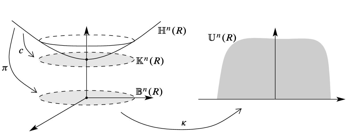
Isometries among the hyperbolic models

 , set
, set  , where
  is the point where the line from the origin to P intersects the hyperplane
  (Fig. 3.4). Because W is characterized as the unique scalar multiple of P whose last coordinate is R, we have
  , and therefore c is given by the formula
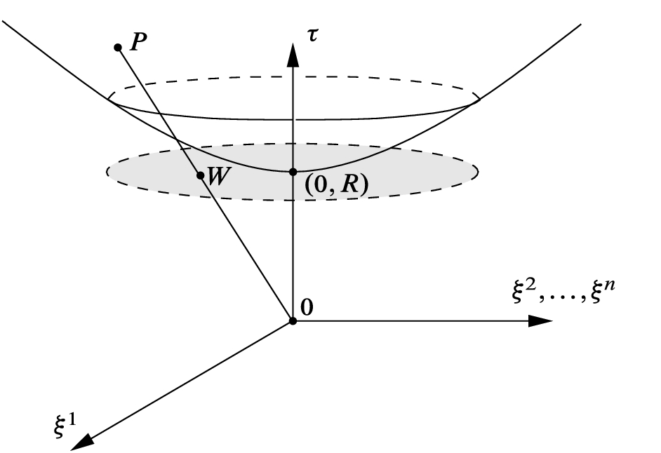
Central projection from the hyperboloid to the Beltrami–Klein model

 guarantees that
  , so c maps
  into
into  . To show that c is a diffeomorphism, we determine its inverse map. Let
  be arbitrary. The unique positive scalar
  such that the point
  lies on
  is characterized by
  , and therefore

 and
and  , we use the fact that
  is the metric induced from
  , analogously to the computation we did for stereographic projection above. With
  defined by (3.12), we have
 .
.
 denote the point
  . For any
  , set
, set  , where
  is the point where the line through S and P intersects the hyperplane
  (Fig. 3.5). The point U is characterized by
  for some nonzero scalar
  , or
, or
Hyperbolic stereographic projection


 because
  . A computation similar to the ones before shows that the inverse map is
 . The computation proceeds just as in the spherical case, so we skip over most of the details:

 . In the 2-dimensional case,
  is easy to write down in complex notation
  and
and  . It is a variant of the classical Cayley transform:
 onto
onto  . Separating z into real and imaginary parts, we can also write this in real terms as
 , and it is easy to check that it maps the upper half-space
  into the ball of radius R. A direct computation shows that its inverse is
 is a diffeomorphism, called the generalized Cayley transform. The verification that
  is basically a long calculation, and is left to Problem 3-4.
We often use the generic notation
 to refer to any one of the Riemannian manifolds of Theorem 3.7, and
  to refer to the corresponding metric; the special case
  is denoted by
 and is called simply hyperbolic space, or in the 2-dimensional case, the hyperbolic plane.
Because all of the models for a given value of R are isometric to each other, when analyzing them geometrically we can use whichever model is most convenient for the application we have in mind. The next corollary is an example in which the Poincaré ball and half-space models serve best.
Corollary 3.8.
Each hyperbolic space is locally conformally flat.
Proof.
In either the Poincaré ball model or the half-space model, the identity map gives a global conformal equivalence with an open subset of Euclidean space. 
The examples presented so far might give the impression that most Riemannian manifolds are locally conformally flat. This is far from the truth, but we do not yet have the tools to prove it. See Problem 8-25 for some explicit examples of Riemannian manifolds that are not locally conformally flat.
The symmetries of  are most easily seen in the hyperboloid model. Let
  denote the group of linear maps from
  to itself that preserve the Minkowski metric, called the
  -dimensional Lorentz group. Note that each element of
  preserves the hyperboloid
  , which has two components determined by
  and
and  . We let
  denote the subgroup of
  consisting of maps that take the
  component of the hyperboloid to itself. (This is called the orthochronous Lorentz group, because physically it represents coordinate changes that preserve the forward time direction.) Then
  preserves
  , and because it preserves
  it acts isometrically on
  . (Problem 5-11 will show that this is the full isometry group.) Recall that
  denotes the set of all orthonormal bases for all tangent spaces of
  .
.
Proposition 3.9.
The group  acts transitively on
  , and therefore
  is frame-homogeneous.
Proof.
 and
and  is an orthonormal basis for
  . Identifying
  with an element of
  in the usual way, we can regard
  as a
as a  -unit vector in
  , and (3.10) shows that it is a scalar multiple of the
  -gradient of the defining function f and thus is orthogonal to
  with respect to
  . Thus
  is a
is a  -orthonormal basis for
  , and
, and  has the following expression in terms of the dual basis
  :
:
 is an element of
  sending
  to p and
  to
to  (Fig. 3.6).
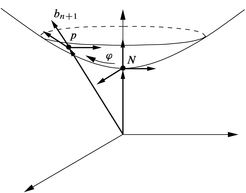
Frame homogeneity of 
Invariant Metrics on Lie Groups
Lie groups provide us with another large class of homogeneous Riemannian manifolds. (See Appendix C for a review of the basic facts about Lie groups that we will use.)
Let G be a Lie group. A Riemannian metric g on G is said to be left-invariant if it is invariant under all left translations:  for all
  . Similarly, g is right-invariant if it is invariant under all right translations, and bi-invariant if it is both left- and right-invariant. The next lemma shows that left-invariant metrics are easy to come by.
Lemma 3.10.
Let G be a Lie group and let  be its Lie algebra of left-invariant vector fields.
- (a)
A Riemannian metric g on G is left-invariant if and only if for all
 , the function g(X, Y) is constant on G.
 - (b)
The restriction map
 together with the natural identification
  gives a bijection between left-invariant Riemannian metrics on G and inner products on
  .
.
 Exercise 3.11. Prove the preceding lemma.
Thus all we need to do to construct a left-invariant metric is choose any inner product on  , and define a metric on G by applying that inner product to left-invariant vector fields. Right-invariant metrics can be constructed in a similar way using right-invariant vector fields. Since a Lie group acts transitively on itself by either left or right translation, every left-invariant or right-invariant metric is homogeneous.
Much more interesting are the bi-invariant metrics, because, as you will be able to prove later (Problems 7-13 and 8-17), their curvatures are intimately related to the structure of the Lie algebra of the group. But bi-invariant metrics are generally much rarer than left-invariant or right-invariant ones; in fact, some Lie groups have no bi-invariant metrics at all (see Problems 3-12 and 3-13). Fortunately, there is a complete answer to the question of which Lie groups admit bi-invariant metrics, which we present in this section.
We begin with a proposition that shows how to determine whether a given left-invariant metric is bi-invariant, based on properties of the adjoint representation of the group. Recall that this is the representation  given by
  , where
  is the automorphism defined by conjugation:
  . See Appendix C for more details.
Proposition 3.12.
Let G be a Lie group and  its Lie algebra. Suppose g is a left-invariant Riemannian metric on G, and let
  denote the corresponding inner product on
  as in Lemma 3.10. Then g is bi-invariant if and only if
  is invariant under the action of
  , in the sense that
  for all
  and
and  .
.
Proof.
 is the associated inner product on
  . Let
. Let  be arbitrary, and note that
  is the composition of left multiplication by
  followed by right multiplication by
  . Thus for every
  , left-invariance implies
  . Therefore, for all
  and
and  , we have
 is invariant under
  . Then the expression on the last line above is equal to
  , which shows that
  . Since this is true for all
  , it follows that g is bi-invariant.
 for each
  , so the above computation yields
 is
is  -invariant.
In order to apply the preceding proposition, we need a lemma about finding invariant inner products on vector spaces. Recall from Appendix C that for every finite-dimensional real vector space V,  denotes the Lie group of all invertible linear maps from V to itself. If H is a subgroup of
  , an inner product
  on V is said to be
  -invariant if
  for all
  and
and  .
.
Lemma 3.13.
Suppose V is a finite-dimensional real vector space and H is a subgroup of  . There exists an H-invariant inner product on V if and only if H has compact closure in
  .
.
Proof.
Assume first that there exists an H-invariant inner product  on V. This implies that H is contained in the subgroup
  consisting of linear isomorphisms of V that are orthogonal with respect to this inner product. Choosing an orthonormal basis of V yields a Lie group isomorphism between
  and
and  (where
  ), so
), so  is compact; and the closure of H is a closed subset of this compact group, and thus is itself compact.
 , and let K denote the closure. A simple limiting argument shows that K is itself a subgroup, and thus it is a Lie group by the closed subgroup theorem (Thm. C.8). Let
  be an arbitrary inner product on V, and let
  be a right-invariant volume form on K (for example, the volume form of some right-invariant metric on K). For fixed
  , define a smooth function
  by
by  . Then define a new inner product
  on V by
 is symmetric and bilinear over
  . For each nonzero
  , we have
  everywhere on K, so
  , showing that
  is indeed an inner product.
 be arbitrary. Then for all
  and
and  , we have
 is right translation by
  . Because
  is right-invariant, it follows from diffeomorphism invariance of the integral that
 is K-invariant, and it is also H-invariant because
  .
. 
Theorem 3.14
(Existence of Bi-invariant Metrics). Let G be a Lie group and  its Lie algebra. Then G admits a bi-invariant metric if and only if
  has compact closure in
  .
.
Proof.
Proposition 3.12 shows that there is a bi-invariant metric on G if and only if there is an  -invariant inner product on
  , and Lemma 3.13 in turn shows that the latter is true if and only if
  has compact closure in
  .
. 
The most important application of the preceding theorem is to compact groups.
Corollary 3.15.
Every compact Lie group admits a bi-invariant Riemannian metric.
Proof.
If G is compact, then  is a compact subgroup of
  because
  is continuous.
Another important application is to prove that certain Lie groups do not admit bi-invariant metrics. One way to do this is to note that if  has compact closure in
  , then every orbit of
  must be a bounded subset of
  with respect to any choice of norm, because it is contained in the image of the compact set
  under a continuous map of the form
  from
from  to
to  . Thus if one can find an element
  and a subset
  such that the elements of the form
  are unbounded in
  for
for  , then there is no bi-invariant metric.
Here are some examples.
Example 3.16
- (a)
Every left-invariant metric on an abelian Lie group is bi-invariant, because the adjoint representation is trivial. Thus the Euclidean metric on
 and the flat metric on
  of Example 2.21 are both bi-invariant.
 - (b)
If a metric g on a Lie group G is left-invariant, then the induced metric on every Lie subgroup
 is easily seen to be left-invariant. Similarly, if g is bi-invariant, then the induced metric on H is bi-invariant.
 - (c)
The Lie group
 (the group of
  real matrices of determinant 1) admits many left-invariant metrics (as does every positive-dimensional Lie group), but no bi-invariant ones. To see this, recall that the Lie algebra of
  is isomorphic to the algebra
  of trace-free
  matrices, and the adjoint representation is given by
  (see Example C.10). If we let
  and
and  for
for  , then
  , which is unbounded as
  . Thus the orbit of
  is not contained in any compact subset, which implies that there is no bi-invariant metric on
  . A similar argument shows that
  admits no bi-invariant metric for any
  . In view of (b) above, this shows also that
  admits no bi-invariant metric for
  . (Of course,
  does admit bi-invariant metrics because it is abelian.)
 - (e)With
 regarded as a submanifold of
  , the map gives a diffeomorphism from
 (3.16)
 to
to  . Under the inverse of this map, the round metric on
  pulls back to a bi-invariant metric on
  , as Problem 3-10 shows.
 - (e)Let
 denote the Lie algebra of
  , identified with the algebra of skew-symmetric
  matrices, and define a bilinear form on
  by This is an
 -invariant inner product, and thus determines a bi-invariant Riemannian metric on
  (see Problem 3-11).
 - (f)
- (g)For
 , the
, the  -dimensional Heisenberg group is the Lie subgroup
  defined by where x and y are treated as column matrices. These are the simplest examples of nilpotent Lie groups, meaning that the series of subgroups
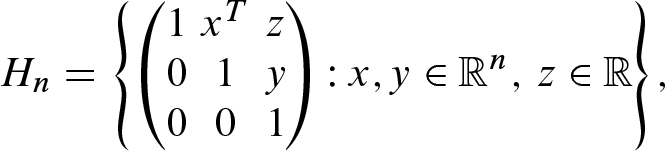
![$$G\supseteq [G,G] \supseteq [G,[G, G]] \supseteq \cdots $$](../images/56724_2_En_3_Chapter/56724_2_En_3_Chapter_TeX_IEq453.png) eventually reaches the trivial subgroup (where for any subgroups
eventually reaches the trivial subgroup (where for any subgroups  , the notation
 ![$$[G_1,G_2]$$](../images/56724_2_En_3_Chapter/56724_2_En_3_Chapter_TeX_IEq456.png) means the subgroup of G generated by all elements of the form
means the subgroup of G generated by all elements of the form  for
for  ). There are many left-invariant metrics on
  , but no bi-invariant ones, as Problem 3-13 shows.
 - (h)Our last example is a group that plays an important role in the classification of 3-manifolds. Let
 denote the following 3-dimensional Lie subgroup of
  : This group is the simplest nonnilpotent example of a solvable Lie group, meaning that the series of subgroups
![$$G\supseteq [G,G] \supseteq [[G,G],[G, G]] \supseteq \cdots $$](../images/56724_2_En_3_Chapter/56724_2_En_3_Chapter_TeX_IEq463.png) eventually reaches the trivial subgroup. Like the Heisenberg groups,
eventually reaches the trivial subgroup. Like the Heisenberg groups,  admits left-invariant metrics but not bi-invariant ones (Problem 3-14). //


In fact, John Milnor showed in 1976 [Mil76] that the only Lie groups that admit bi-invariant metrics are those that are isomorphic to direct products of compact groups and abelian groups.
Other Homogeneous Riemannian Manifolds
There are many homogeneous Riemannian manifolds besides the frame-homogeneous ones and the Lie groups with invariant metrics. To identify other examples, it is natural to ask the following question: If M is a smooth manifold endowed with a smooth, transitive action by a Lie group G (called a homogeneous G-space or just a homogeneous space), is there a Riemannian metric on M that is invariant under the group action?
The next theorem gives a necessary and sufficient condition for existence of an invariant Riemannian metric that is usually easy to check.
Theorem 3.17
(Existence of Invariant Metrics on Homogeneous Spaces). Suppose G is a Lie group and M is a homogeneous G-space. Let  be a point in M, and let
  denote the isotropy representation at
  . There exists a G-invariant Riemannian metric on M if and only if
  has compact closure in
  .
.
Proof.
Assume first that g is a G-invariant metric on M. Then the inner product  on
on  is invariant under the isotropy representation, so it follows from Lemma 3.13 that
  has compact closure in
  .
.
 has compact closure in
  . Lemma 3.13 shows that there is an inner product
  on
on  that is invariant under the isotropy representation. For arbitrary
  , we define an inner product
  on
on  by choosing an element
  such that
  and setting
 are any two such elements of G, then
  with
with  , so
, so
 given by
  is a smooth surjection because the action is smooth and transitive. Given
  , if we let
  denote the map
  and
and  the left translation by
  , then the map
  satisfies
 on G by
  . (It will typically not be positive definite, because
  if either v or w is tangent to the isotropy group
  and thus in the kernel of
  .) For all
  , (3.17) implies
 is a left-invariant tensor field on G. Every basis
  for the Lie algebra of G forms a smooth global left-invariant frame for G, and with respect to such a frame the components
  are constant; thus
  is a smooth tensor field on G.
 , the fact that
  is a surjective smooth submersion implies that there exist a neighborhood U of p and a smooth local section
  (Thm. A.17). Then

The next corollary, which follows immediately from Theorem 3.17, addresses the most commonly encountered case. (Other necessary and sufficient conditions for the existence of invariant metrics are given in [Poo81, 6.58–6.59].)
Corollary 3.18.
If a Lie group G acts smoothly and transitively on a smooth manifold M with compact isotropy groups, then there exists a G-invariant Riemannian metric on M. 
 Exercise 3.19. Suppose G is a Lie group and M is a homogeneous G-space that admits at least one g-invariant metric. Show that for each
  , the map
  gives a bijection between G-invariant metrics on M and
  -invariant inner products on
  .
.
Locally Homogeneous Riemannian Manifolds
A Riemannian manifold (M, g) is said to be locally homogeneous if for every pair of points  there is a Riemannian isometry from a neighborhood of p to a neighborhood of q that takes p to q. Similarly, we say that (M, g) is locally frame-homogeneous if for every
  and every pair of orthonormal bases
  for
for  and
and  for
for  , there is an isometry from a neighborhood of p to a neighborhood of q that takes p to q, and whose differential takes
  to
to  for each i.
Every homogeneous Riemannian manifold is locally homogeneous, and every frame-homogeneous one is locally frame-homogeneous. Every proper open subset of a homogeneous or frame-homogeneous Riemannian manifold is locally homogeneous or locally frame-homogeneous, respectively. More interesting examples arise in the following way.
Proposition 3.20.
Suppose  is a homogeneous Riemannian manifold, (M, g) is a Riemannian manifold, and
  is a Riemannian covering. Then (M, g) is locally homogeneous. If
  is frame-homogeneous, then (M, g) is locally frame-homogeneous.
 Exercise 3.21. Prove this proposition.
Locally homogeneous Riemannian metrics play an important role in classification theorems for manifolds, especially in low dimensions. The most fundamental case is that of compact 2-manifolds, for which we have the following important theorem.
Theorem 3.22
(Uniformization of Compact Surfaces). Every compact, connected, smooth 2-manifold admits a locally frame-homogeneous Riemannian metric, and a Riemannian covering by the Euclidean plane, hyperbolic plane, or round unit sphere.
Sketch of proof. The proof relies on the topological classification of compact surfaces (see, for example, [LeeTM, Thms. 6.15 and 10.22]), which says that every connected compact surface is homeomorphic to a sphere, a connected sum of one or more tori, or a connected sum of one or more projective planes. The crux of the proof is showing that each of the model surfaces on this list has a metric that admits a Riemannian covering by one of the model frame-homogeneous manifolds, and therefore is locally frame-homogeneous by Proposition 3.20. We consider each model surface in turn.
The 2-sphere:  , of course, has its round metric, and the identity map is a Riemannian covering.
The 2-torus: Exercise 2.36 shows that the flat metric on  described in Example 2.21 admits a Riemannian covering by
  .
.
 copies of
  : It is shown in [LeeTM, Example 6.13] that such a surface is homeomorphic to a quotient of a regular 4n-sided polygonal region by side identifications indicated schematically by the sequence of labels
  (Fig. 3.7 illustrates the case
  ). Let
  be the following subgroup:
A connected sum of tori

Constructing a Riemannian covering

 , there is a discrete subgroup
  such that the quotient map
  is a covering map, and
  is homeomorphic to a connected sum of n tori. The group is found by first identifying a compact region
  bounded by a “regular geodesic polygon," which is a union of 4n congruent circular arcs making interior angles that all measure exactly
  , so that 4n of them fit together locally to fill out a neighborhood of a point (see Fig. 3.8). (The name “geodesic polygon" reflects the fact that these circular arcs are segments of geodesics with respect to the hyperbolic metric, as we will see in Chapter 5.) Then
  is the group generated by certain elements of G that take an edge with a label
  or
or  to the other edge with the same label. Because
  acts isometrically, it follows that such a connected sum admits a locally frame-homogeneous metric and a Riemannian covering by the Poincaré disk. For details, see the proofs of Theorems 12.29 and 12.30 of [LeeTM].
The projective plane: Example 2.34 shows that  has a metric that admits a 2-sheeted Riemannian covering by
  .
.
 : It is shown in [LeeTM, Lemma 6.16] that
  is homeomorphic to the Klein bottle, which is the quotient space of the unit square
 ![$$[0,1]\times [0,1]$$](../images/56724_2_En_3_Chapter/56724_2_En_3_Chapter_TeX_IEq548.png) by the equivalence relation generated by the following relations (see Fig. 3.9):
by the equivalence relation generated by the following relations (see Fig. 3.9):
The Klein bottle

Connected sum of three projective planes

 be the Euclidean group in two dimensions as defined earlier in this chapter, and let
  be the subgroup defined by
 acts freely and properly on
  , and every
  -orbit has a representative in the unit square such that two points in the square are in the same orbit if and only if they satisfy the equivalence relation generated by the relations in (3.19). Thus the orbit space
  is homeomorphic to the Klein bottle, and since the group action is isometric, it follows that the Klein bottle inherits a flat, locally frame-homogeneous metric and the quotient map is a Riemannian covering. Problem 3-18 asks you to work out the details.
A connected sum of  copies of
  : Such a surface is homeomorphic to a quotient of a regular 2n-sided polygonal region by side identifications according to
  [LeeTM, Example 6.13]. As in the case of a connected sum of tori, there is a compact region
  bounded by a 2n-sided regular geodesic polygon whose interior angles are all
  (see Fig. 3.10), and there is a discrete group of isometries that realizes the appropriate side identifications and yields a quotient homeomorphic to the connected sum. The new ingredient here is that because such a connected sum is not orientable, we must work with the full group of isometries of
  , not just the (orientation-preserving) ones determined by elements of G; but otherwise the argument is essentially the same as the one for connected sums of tori. The details can be found in [Ive92, Section VII.1].
There is one remaining step. The arguments above show that each compact topological 2-manifold possesses a smooth structure and a locally frame-homogeneous Riemannian metric, which admits a Riemannian covering by one of the three frame-homogeneous model spaces. However, we started with a smooth compact 2-manifold, and we are looking for a Riemannian metric that is smooth with respect to the given smooth structure. To complete the proof, we appeal to a result by James Munkres [Mun56], which shows that any two smooth structures on a 2-manifold are related by a diffeomorphism; thus after pulling back the metric by this diffeomorphism, we obtain a locally frame-homogeneous metric on M with its originally given smooth structure. 
 with the Euclidean metric
 with a round metric
 with a hyperbolic metric
 with a product of a round metric and the Euclidean metric
 with a product of a hyperbolic metric and the Euclidean metric
The Heisenberg group
 of Example 3.16(g) with a left-invariant metric
The group
 of Example 3.16(h) with a left-invariant metric
The universal covering group of
 with a left-invariant metric
The Thurston geometrization conjecture was proved in 2003 by Grigori Perelman. The proof is described in several books [BBBMP, KL08, MF10, MT14].
Symmetric Spaces
We end this section with a brief introduction to another class of Riemannian manifolds with abundant symmetry, called symmetric spaces. They turn out to be intermediate between frame-homogeneous and homogeneous Riemannian manifolds.
Here is the definition. If (M, g) is a Riemannian manifold and  , a point reflection at p is an isometry
  that fixes p and satisfies
  . A Riemannian manifold (M, g) is called a (Riemannian) symmetric space if it is connected and for each
  there exists a point reflection at p. (The modifier “Riemannian" is included to distinguish such spaces from other kinds of symmetric spaces that can be defined, such as pseudo-Riemannian symmetric spaces and affine symmetric spaces; since we will be concerned only with Riemannian symmetric spaces, we will sometimes refer to them simply as “symmetric spaces" for brevity.)
Although we do not yet have the tools to prove it, we will see later that every Riemannian symmetric space is homogeneous (see Problem 6-19). More generally, (M, g) is called a ( Riemannian) locally symmetric space if each  has a neighborhood U on which there exists an isometry
  that is a point reflection at p. Clearly every Riemannian symmetric space is locally symmetric.
The next lemma can be used to facilitate the verification that a given Riemannian manifold is symmetric.
Lemma 3.23.
If (M, g) is a connected homogeneous Riemannian manifold that possesses a point reflection at one point, then it is symmetric.
Proof.
 be a point reflection at
  . Given any other point
  , by homogeneity there is an isometry
  satisfying
  . Then
  is an isometry that fixes q. Because
  is linear, it commutes with multiplication by
  , so
, so
 is a point reflection at q.
Example 3.24
- (a)
Suppose (M, g) is any connected frame-homogeneous Riemannian manifold. Then for each
 , we can choose an orthonormal basis
  for
for  , and frame homogeneity guarantees that there is an isometry
  that fixes p and sends
  to
to  , which implies that
  . Thus every frame-homogeneous Riemannian manifold is a symmetric space. In particular, all Euclidean spaces, spheres, and hyperbolic spaces are symmetric.
 - (b)Suppose G is a connected Lie group with a bi-invariant Riemannian metric g. If we define
 by
by  , then it is straightforward to check that
  for every
  , from which it follows that
  . To see that
  is an isometry, let
  be arbitrary. The identity
  for all
  implies that
  , and therefore it follows from bi-invariance of g that Therefore
 is an isometry of g and hence a point reflection at e. Lemma 3.23 then implies that (G, g) is a symmetric space.
 - (c)
The complex projective spaces introduced in Example 2.30 and the Grassmann manifolds introduced in Problem 2-7 are all Riemannian symmetric spaces (see Problems 3-19 and 3-20).
- (d)
Every product of Riemannian symmetric spaces is easily seen to be a symmetric space when endowed with the product metric. A symmetric space is said to be irreducible if it is not isometric to a product of positive-dimensional symmetric spaces. //
Model Pseudo-Riemannian Manifolds
The definitions of the Euclidean, spherical, and hyperbolic metrics can easily be adapted to give analogous classes of frame-homogeneous pseudo-Riemannian manifolds.
The first example is one we have already seen: the pseudo-Euclidean space of signature  is the pseudo-Riemannian manifold
 , where
  is the pseudo-Riemannian metric defined by (2.24).
 and the pseudohyperbolic space
  as follows. As manifolds,
 and
and  are defined by
 on
on  , and
, and  on
on  .
.Theorem 3.25.
For all r, s, and R as above,  and
and  are pseudo-Riemannian manifolds of signature (r, s).
Proof.
Problem 3-22. 
It turns out that these pseudo-Riemannian manifolds all have the same degree of symmetry as the three classes of model Riemannian manifolds introduced earlier. For pseudo-Riemannian manifolds, though, it is necessary to modify the definition of frame homogeneity slightly. If (M, g) is a pseudo-Riemannian manifold of signature (r, s), let us say that an orthonormal basis for some tangent space  is in standard order if the expression for
  in terms of the dual basis
  is
is  , with all positive terms coming before the negative terms. With this understanding, we define
  to be the set of all standard-ordered orthonormal bases for all tangent spaces to M, and we say that (M, g) is frame-homogeneous if the isometry group acts transitively on
  .
.
Theorem 3.26.
All pseudo-Euclidean spaces, pseudospheres, and pseudohyperbolic spaces are frame-homogeneous.
Proof.
Problem 3-23. 
In the particular case of signature (n, 1), the Lorentz manifolds  and
and  are called de Sitter space of radius
  and anti-de Sitter space of radius
  , respectively.
Problems
- 3-1.
Show that (3.2) defines a smooth isometric action of
 on
on  , and the induced action on
  is transitive. (Used on p. 57.)
 - 3-2.
Prove that the metric on
 described in Example 2.34 is frame-homogeneous. (Used on p. 145)
 - 3-3.
Prove Proposition 3.1 (about homogeneous and isotropic Riemannian manifolds).
- 3-4.
Complete the proof of Theorem 3.7 by showing that
 .
. - 3-5.
- (a)
Prove that
 is isometric to
  for each
  .
. - (b)
Prove that
 is isometric to
  for each
  .
. - (c)
We could also have defined a family of metrics on
 by
by  . Why did we not bother?
(Used on p. 185.)
- (a)
- 3-6.
Show that two Riemannian metrics
 and
and  are conformal if and only if they define the same angles but not necessarily the same lengths, and that a diffeomorphism is a conformal equivalence if and only if it preserves angles. [Hint: Let
  be a local orthonormal frame for
  , and consider the
  -angle between
  and
and  .] (Used on p. 59.)
 - 3-7.Let
 denote the upper half-plane model of the hyperbolic plane (of radius 1), with the metric
  . Let
. Let  denote the group of
  real matrices of determinant 1. Regard
  as a subset of the complex plane with coordinate
  , and let Show that this defines a smooth, transitive, orientation-preserving, and isometric action of
 on
on  . Is the induced action transitive on
  ?
? - 3-8.Let
 denote the Poincaré disk model of the hyperbolic plane (of radius 1), with the metric
  , and let
  be the subgroup defined by (3.18). Regarding
  as a subset of the complex plane with coordinate
  , let G act on
  by Show that this defines a smooth, transitive, orientation-preserving, and isometric action of G on
 . [Hint: One way to proceed is to define an action of G on the upper half-plane by
  , where
  is the Cayley transform defined by (3.14) in the case
  , and use the result of Problem 3-7.] (Used on pp. 73, 185.)
 - 3-9.
Suppose G is a compact Lie group with a left-invariant metric g and a left-invariant orientation. Show that the Riemannian volume form
 is bi-invariant. [Hint: Show that
  is equal to the Riemannian volume form for a bi-invariant metric.]
 - 3-10.Consider the basisfor the Lie algebra

 . For each positive real number a, define a left-invariant metric
  on the group
  by declaring X, Y, aZ to be an orthonormal frame.
- (a)
Show that
 is bi-invariant if and only if
  .
. - (b)
Show that the map defined by (3.16) is an isometry between
 and
and  . [Remark:
  with any of these metrics is called a Berger sphere, named after Marcel Berger.]
(Used on pp. 56, 71, 259.)
- (a)
- 3-11.
Prove that the formula
 defines a bi-invariant Riemannian metric on
  . (See Example 3.16(e).)
 - 3-12.
Regard the upper half-space
 as a Lie group as described in Example 3.16(f).
- (a)
Show that for each
 , the hyperbolic metric
  on
on  is left-invariant.
 - (b)
Show that
 does not admit any bi-invariant metrics.
(Used on pp. 68, 72.)
- (a)
- 3-13.
Write down an explicit formula for an arbitrary left-invariant metric on the Heisenberg group
 of Example 3.16(g) in terms of global coordinates
  , and show that the group has no bi-invariant metrics. (Used on pp. 68, 72.)
 - 3-14.
- 3-15.Let
 be the
  -dimensional Minkowski space with coordinates
  and with the Minkowski metric
  . Let
. Let  be the set
- (a)
Prove that S is a smooth submanifold diffeomorphic to
 , and with the induced metric
  it is isometric to the round unit
  -sphere.
 - (b)
Define an action of the orthochronous Lorentz group
 on S as follows: For every
  , let
, let  denote the 1-dimensional subspace of
  spanned by p. Given
  , show that the image set
  is a 1-dimensional subspace that intersects S in exactly one point, so we can define
  to be the unique point in
  . Prove that this is a smooth transitive action on S.
 - (c)
Prove that
 acts by conformal diffeomorphisms of (S, g).
- (a)
- 3-16.
Prove that there is no Riemannian metric on the sphere that is invariant under the group action described in Problem 3-15.
- 3-17.Given a Lie group G, define an action of the product group
 on G by
  . Show that this action is transitive, and that the isotropy group of the identity is the diagonal subgroup
  . Then show that the following diagram commutes: where
 is the isotropy representation of
  and
and  is the Lie algebra of G, and use this to give an alternative proof of Theorem 3.14.
 - 3-18.
Let
 be the subgroup defined by (3.20). Prove that
  acts freely and properly on
  and the orbit space is homeomorphic to the Klein bottle, and conclude that the Klein bottle has a flat metric and a Riemannian covering by the Euclidean plane.
 - 3-19.
Show that the Fubini–Study metric on
 (Example 2.30) is homogeneous, isotropic, and symmetric. (Used on p. 78.)
 - 3-20.
Show that the metric on the Grassmannian
 defined in Problem 2-7 is homogeneous, isotropic, and symmetric. (Used on p. 78.)
 - 3-21.
Let
 be a simply connected Riemannian manifold, and suppose
  and
and  are countable subgroups of
  acting smoothly, freely, and properly on M (when endowed with the discrete topology). For
  , let
, let  , and let
  be the Riemannian metric on
  that makes the quotient map
  a Riemannian covering (see Prop. 2.32). Prove that the Riemannian manifolds
  and
and  are isometric if and only if
  and
and  are conjugate subgroups of
  .
. - 3-22.
Prove Theorem 3.25 (showing that pseudospheres and pseudohyperbolic spaces are pseudo-Riemannian manifolds). [Hint: Mimic the argument in the proof of Theorem 3.7 that
 is Riemannian.]
 - 3-23.
Prove Theorem 3.26 (pseudo-Euclidean spaces, pseudospheres, and pseudohyperbolic spaces are frame-homogeneous).
- 3-24.Prove that for all positive integers r and s and every real number
 , both the pseudohyperbolic space
  and the pseudosphere
  are diffeomorphic to
  . [Hint: Consider the maps
  given by
 ![$$\begin{aligned} \varphi (x, y) = \left( Rx, \big ( \sqrt{1+|x|^2}\big )Ry\right) , \quad \psi (x, y) = \left( \big ( \sqrt{1+|x|^2}\big )Ry, Rx\right) .] \end{aligned}$$](../images/56724_2_En_3_Chapter/56724_2_En_3_Chapter_TeX_Equ58.png)
- 3-25.Let
 be the r-dimensional ball of radius R with the Beltrami–Klein metric (3.9), and let
  be the product manifold
  with the pseudo-Riemannian warped product metric
  , where
  is given by Define
 by Prove that the image of F is the anti-de Sitter space
 , and F defines a pseudo-Riemannian covering of
  by
by  . [Remark: We are tacitly extending the notions of warped product metric and Riemannian coverings to the pseudo-Riemannian case in the obvious ways. It follows from the result of Problem 3-24 that
  is simply connected when
  but
but  is not. This shows that
  , called universal anti-de Sitter space of radius R, is the universal pseudo-Riemannian covering manifold of
  .]
.]
