Riemannian Submanifolds

This chapter has a dual purpose: first to apply the theory of curvature to Riemannian submanifolds, and then to use these concepts to derive a precise quantitative interpretation of the curvature tensor.

After introducing some basic definitions and terminology concerning Riemannian submanifolds, we define a vector-valued bilinear form called the second fundamental form, which measures the way a submanifold curves within the ambient manifold. We then prove the fundamental relationships between the intrinsic and extrinsic geometries of a submanifold, including the Gauss formula, which relates the Riemannian connection on the submanifold to that of the ambient manifold, and the Gauss equation, which relates their curvatures. We then show how the second fundamental form measures the extrinsic curvature of submanifold geodesics.

Using these tools, we focus on the special case of hypersurfaces, and use the second fundamental form to define some real-valued curvature quantities called the principal curvatures, mean curvature, and Gaussian curvature. Specializing even more to hypersurfaces in Euclidean space, we describe various concrete geometric interpretations of these quantities. Then we prove Gauss’s Theorema Egregium, which shows that the Gaussian curvature of a surface in $\mathbb {R}^3$ can be computed intrinsically from the curvature tensor of the induced metric.

In the last section, we introduce the promised quantitative geometric interpretation of the curvature tensor. It allows us to compute sectional curvatures, which are just the Gaussian curvatures of 2-dimensional submanifolds swept out by geodesics tangent to 2-planes in the tangent space. Finally, we compute the sectional curvatures of our frame-homogeneous model Riemannian manifolds—Euclidean spaces, spheres, and hyperbolic spaces.

The Second Fundamental Form

Suppose (M, g) is a Riemannian submanifold of a Riemannian manifold $\big ({{\widetilde{M}}},{\tilde{g}}\big )$ . Recall that this means that M is a submanifold of ${{\widetilde{M}}}$ endowed with the induced metric $g = \iota _M^* {\tilde{g}}$ (where $\iota _M:M\mathrel {\hookrightarrow }{{\widetilde{M}}}$ is the inclusion map). Our goal in this chapter is to study the relationship between the geometry of M and that of ${{\widetilde{M}}}$ .

Although we focus our attention in this chapter on embedded submanifolds for simplicity, the results we present are all local, so they apply in much greater generality. In particular, if $M\subseteq {{\widetilde{M}}}$ is an immersed submanifold, then every point of M has a neighborhood in M that is embedded in ${{\widetilde{M}}}$ , so the results of this chapter can be applied by restricting to such a neighborhood. Even more generally, if (M, g) is any Riemannian manifold and $F:M\mathrel {\rightarrow }{{\widetilde{M}}}$ is an isometric immersion (meaning that $F^*\tilde{g}=g$ ), then again every point $p\in M$ has a neighborhood $U\subseteq M$ such that $$F|_U$$ is an embedding, so the results apply to $F(U)\subseteq M$ . We leave it to the reader to sort out the minor modifications in notation and terminology needed to handle these more general situations.

The results in the first section of this chapter apply virtually without modification to Riemannian submanifolds of pseudo-Riemannian manifolds (ones on which the induced metric is positive definite), so we state most of our theorems in that case. Recall that when the ambient metric ${\tilde{g}}$ is indefinite, this includes the assumption that the induced metric $g=\iota _M^*{\tilde{g}}$ is positive definite. Some of the results can also be extended to pseudo-Riemannian submanifolds of mixed signature, but there are various pitfalls to watch out for in that case; so for simplicity we restrict to the case of Riemannian submanifolds. See [dC92] for a thorough treatment of pseudo-Riemannian submanifolds.

Also, most of these results can be adapted to manifolds and submanifolds with boundary, simply by embedding everything in slightly larger manifolds without boundary, but one might need to be careful about the statements of some of the results when the submanifold intersects the boundary. Since the interaction of submanifolds with boundaries is not our primary concern here, for simplicity we state all of these results in the case of empty boundary only.

Throughout this chapter, therefore, we assume that $\big ({{\widetilde{M}}},\tilde{g}\big )$ is a Riemannian or pseudo-Riemannian manifold of dimension m, and (M, g) is an embedded n-dimensional Riemannian submanifold of ${{\widetilde{M}}}$ . We call ${{\widetilde{M}}}$ the ambient manifold. We will denote covariant derivatives and curvatures associated with (M, g) in the usual way ( $\nabla$ , R, $$ Rm $$ , etc.), and write those associated with $\big ({{\widetilde{M}}},{\tilde{g}}\big )$ with tildes ( $\tilde{\nabla }$ , $\tilde{R}$ , $\widetilde{ Rm }$ , etc.). We can unambiguously use the inner product notation $\langle v, w\rangle$ to refer either to g or to ${\tilde{g}}$ , since g is just the restriction of ${\tilde{g}}$ to pairs of vectors in TM.

Our first main task is to compare the Levi-Civita connection of M with that of ${{\widetilde{M}}}$ . The starting point for doing so is the orthogonal decomposition of sections of the ambient tangent bundle $T{{\widetilde{M}}}|_M$ into tangential and orthogonal components. Just as we did for submanifolds of $\mathbb {R}^n$ in Chapter 4, we define orthogonal projection maps called tangential and normal projections :

$\begin{aligned} \begin{aligned} \pi ^\top&:T{{\widetilde{M}}}|_M\mathrel {\rightarrow }TM,\\ \pi ^\perp&:T{{\widetilde{M}}}|_M\mathrel {\rightarrow }N{ M}. \end{aligned} \end{aligned}$

In terms of an adapted orthonormal frame $(E_1,\dots , E_m)$ for M in ${{\widetilde{M}}}$ , these are just the usual projections onto $\mathrm{span}(E_1,\dots , E_n)$ and $\mathrm{span}(E_{n+1},\dots , E_m)$ respectively, so both projections are smooth bundle homomorphisms (i.e., they are linear on fibers and map smooth sections to smooth sections). If X is a section of $T{{\widetilde{M}}}|_M$ , we often use the shorthand notations $X^\top = \pi ^\top X$ and $X^\perp = \pi ^\perp X$ for its tangential and normal projections.

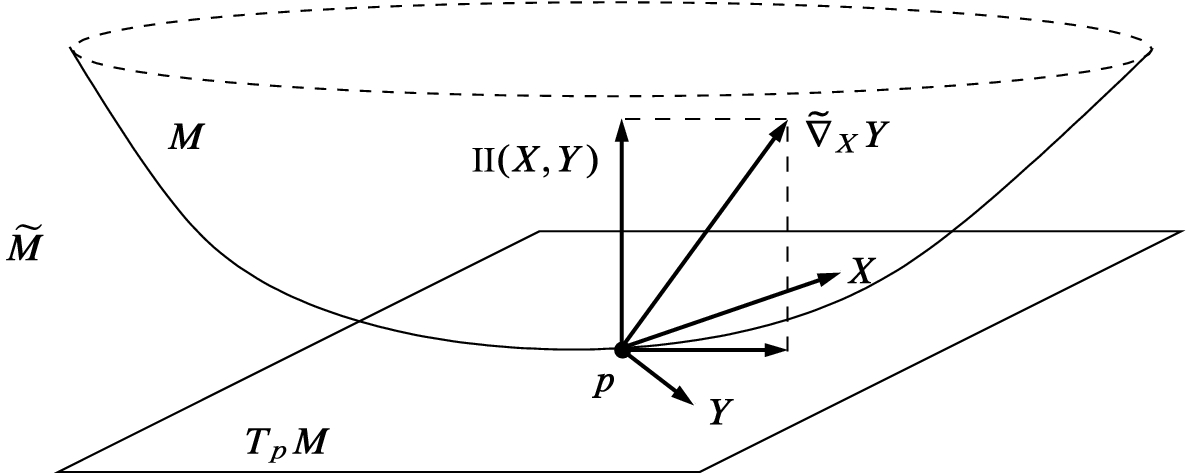
If X, Y are vector fields in $\mathfrak X(M)$ , we can extend them to vector fields on an open subset of ${{\widetilde{M}}}$ (still denoted by X and Y), apply the ambient covariant derivative operator ${\tilde{\nabla }}$ , and then decompose at points of M to get

$\begin{aligned} \tilde{\nabla }_XY = \big (\tilde{\nabla }_XY \big )^\top + \big (\tilde{\nabla }_XY \big )^\perp . \end{aligned}$

(8.1)

We wish to interpret the two terms on the right-hand side of this decomposition.

Let us focus first on the normal component. We define the second fundamental form of $\varvec{M}$ to be the map $\mathrm {II}:\mathfrak X(M)\times \mathfrak X(M)\mathrel {\rightarrow }\varGamma (NM)$ (read “two”) given by

$\begin{aligned} \mathrm {II}(X, Y) = \big (\tilde{\nabla }_{ X} Y\big )^\perp , \end{aligned}$

where X and Y are extended arbitrarily to an open subset of ${{\widetilde{M}}}$ (Fig. 8.1). Since $\pi ^\perp$ maps smooth sections to smooth sections, $\mathrm {II}(X, Y)$ is a smooth section of $$N{ M}$$

../images/56724_2_En_8_Chapter/56724_2_En_8_Fig1_HTML.png — Fig. 8.1:
The second fundamental form

The term first fundamental form , by the way, was originally used to refer to the induced metric g on M. Although that usage has mostly been replaced by more descriptive terminology, we seem unfortunately to be stuck with the name “second fundamental form.” The word “form” in both cases refers to bilinear form, not differential form.

Proposition 8.1

(Properties of the Second Fundamental Form). Suppose (M, g) is an embedded Riemannian submanifold of a Riemannian or pseudo-Riemannian manifold $\big ({{\widetilde{M}}},{\tilde{g}}\big )$ , and let $X, Y\in \mathfrak X(M)$ .

(a)
$\mathrm {II}(X, Y)$ is independent of the extensions of X and Y to an open subset of ${{\widetilde{M}}}$ .
(b)
$\mathrm {II}(X, Y)$ is bilinear over $C^\infty (M)$ in X and Y.
(c)
$\mathrm {II}(X, Y)$ is symmetric in X and Y.
(d)
The value of $\mathrm {II}(X, Y)$ at a point $p\in M$ depends only on and .

Proof.

Choose particular extensions of X and Y to a neighborhood of M in ${{\widetilde{M}}}$ , and for simplicity denote the extended vector fields also by X and Y. We begin by proving that $\mathrm {II}(X, Y)$ is symmetric in X and Y when defined in terms of these extensions. The symmetry of the connection ${\tilde{\nabla }}$ implies

$\begin{aligned} \mathrm {II}(X,Y) - \mathrm {II}(Y,X) = \big ({\tilde{\nabla }}_XY - {\tilde{\nabla }}_YX\big )^\perp =[X, Y]^\perp . \end{aligned}$

Since X and Y are tangent to M at all points of M, so is their Lie bracket (Cor. A.40). Therefore $[X, Y]^\perp =0$ , so $\mathrm {II}$ is symmetric.

Because ${\tilde{\nabla }}_{X}Y|_p$ depends only on $$X_p$$ , it follows that the value of $\mathrm {II}(X, Y)$ at p depends only on $$X_p$$ , and in particular is independent of the extension chosen for X. Because ${\tilde{\nabla }}_{X}Y$ is linear over $C^\infty \bigl ({{\widetilde{M}}}\bigr )$ in X, and every $f\in C^\infty (M)$ can be extended to a smooth function on a neighborhood of M in ${{\widetilde{M}}}$ , it follows that $\mathrm {II}(X, Y)$ is linear over $C^\infty (M)$ in X. By symmetry, the same claims hold for Y. $\square$

As a consequence of the preceding proposition, for every $p\in M$ and all vectors $v, w\in T_pM$ , it makes sense to interpret $\mathrm {II}(v, w)$ as the value of $\mathrm {II}(V, W)$ at p, where V and W are any vector fields on M such that $$V_p=v$$ and $$W_p=W$$ , and we will do so from now on without further comment.

We have not yet identified the tangential term in the decomposition of ${\tilde{\nabla }}_XY$ . Proposition 5.12(b) showed that in the special case of a submanifold of a Euclidean or pseudo-Euclidean space, it is none other than the covariant derivative with respect to the Levi-Civita connection of the induced metric on M. The following theorem shows that the same is true in the general case. Therefore, we can interpret the second fundamental form as a measure of the difference between the intrinsic Levi-Civita connection on M and the ambient Levi-Civita connection on ${{\widetilde{M}}}$ .

Theorem 8.2

(The Gauss Formula). Suppose (M, g) is an embedded Riemannian submanifold of a Riemannian or pseudo-Riemannian manifold $\big ({{\widetilde{M}}},{\tilde{g}}\big )$ . If $X, Y\in \mathfrak X(M)$ are extended arbitrarily to smooth vector fields on a neighborhood of M in ${{\widetilde{M}}}$ , the following formula holds along M:

$\begin{aligned} {\tilde{\nabla }}_XY = \nabla _XY + \mathrm {II}(X, Y). \end{aligned}$

Proof.

Because of the decomposition (8.1) and the definition of the second fundamental form, it suffices to show that $\big ({\tilde{\nabla }}_XY\big ){}^\top = \nabla _XY$ at all points of M.

Define a map $\nabla ^\top :\mathfrak X(M)\times \mathfrak X(M)\mathrel {\rightarrow }\mathfrak X(M)$ by

$\begin{aligned} \nabla ^\top _XY = \big ({\tilde{\nabla }}_XY\big )^\top , \end{aligned}$

where X and Y are extended arbitrarily to an open subset of ${{\widetilde{M}}}$ . We examined a special case of this construction, in which ${\tilde{g}}$ is a Euclidean or pseudo-Euclidean metric, in Example 4.9. It follows exactly as in that example that $\nabla ^\top$ is a connection on M, and exactly as in the proofs of Propositions 5.8 and 5.9 that it is symmetric and compatible with g. The uniqueness of the Riemannian connection on M then shows that $\nabla ^\top =\nabla$ . $\square$

The Gauss formula can also be used to compare intrinsic and extrinsic covariant derivatives along curves. If $\gamma :I\mathrel {\rightarrow }M$ is a smooth curve and X is a vector field along $\gamma$ that is everywhere tangent to M, then we can regard X as either a vector field along $\gamma$ in ${{\widetilde{M}}}$ or a vector field along $\gamma$ in M. We let $\tilde{D}_tX$ and $$D_tX$$ denote its covariant derivatives along $\gamma$ as a curve in ${{\widetilde{M}}}$ and as a curve in M, respectively. The next corollary shows how the two covariant derivatives are related.

Corollary 8.3

(The Gauss Formula Along a Curve). Suppose (M, g) is an embedded Riemannian submanifold of a Riemannian or pseudo-Riemannian manifold $\big ({{\widetilde{M}}},{\tilde{g}}\big )$ , and $\gamma :I\mathrel {\rightarrow }M$ is a smooth curve. If X is a smooth vector field along $\gamma$ that is everywhere tangent to M, then

$\begin{aligned} {\tilde{D}_t X} = {D_t X} + \mathrm {II}\left( \gamma ', X\right) . \end{aligned}$

(8.2)

Proof.

For each $t_0\in I$ , we can find an adapted orthonormal frame $(E_1,\dots , E_m)$ in a neighborhood of $\gamma (t_0)$ . (Recall that our default assumption is that $\dim {{\widetilde{M}}}=m$ and $\dim M=n$ .) In terms of this frame, X can be written $X(t) = \sum _{i=1}^n X^i(t)E_i|_{\gamma (t)}$ . Applying the product rule and the Gauss formula, and using the fact that each vector field $$E_i$$

is extendible, we get

../images/56724_2_En_8_Chapter/56724_2_En_8_Equ110_HTML.png

Although the second fundamental form is defined in terms of covariant derivatives of vector fields tangent to M, it can also be used to evaluate extrinsic covariant derivatives of normal vector fields, as the following proposition shows. To express it concisely, we introduce one more notation. For each normal vector field $N\in \varGamma (NM)$ , we obtain a scalar-valued symmetric bilinear form $\mathrm {II}_N:\mathfrak X(M)\times \mathfrak X(M)\mathrel {\rightarrow }C^\infty (M)$ by

$\begin{aligned} \mathrm {II}_N (X,Y) = \langle N,\mathrm {II}(X, Y)\rangle . \end{aligned}$

(8.3)

Let $W_N:\mathfrak X(M)\mathrel {\rightarrow }\mathfrak X(M)$ denote the self-adjoint linear map associated with this bilinear form, characterized by

$\begin{aligned} \langle W_N(X), Y\rangle = \mathrm {II}_N(X,Y) = \langle N,\mathrm {II}(X, Y)\rangle . \end{aligned}$

(8.4)

The map

is called the Weingarten map in the direction of ${\varvec{N}}$ . Because the second fundamental form is bilinear over $C^\infty (M)$ , it follows that $$W_N$$

is linear over $C^\infty (M)$ and thus defines a smooth bundle homomorphism from TM to itself.

Proposition 8.4

(The Weingarten Equation). Suppose (M, g) is an embedded Riemannian submanifold of a Riemannian or pseudo-Riemannian manifold $\big ({{\widetilde{M}}},{\tilde{g}}\big )$ . For every $X\in \mathfrak X(M)$ and $N\in \varGamma (NM)$ , the following equation holds:

$\begin{aligned} \big ({\tilde{\nabla }}_X N \big )^\top = -W_{N}(X), \end{aligned}$

(8.5)

when N is extended arbitrarily to an open subset of ${{\widetilde{M}}}$ .

Proof.

Note that at points of M, the covariant derivative ${\tilde{\nabla }}_X N$ is independent of the choice of extensions of X and N by Proposition 4.26. Let $Y\in \mathfrak X(M)$ be arbitrary, extended to a vector field on an open subset of ${{\widetilde{M}}}$ . Since $\langle N, Y\rangle$ vanishes identically along M and X is tangent to M, the following holds at points of M:

$\begin{aligned} \begin{aligned} 0&= X\langle N,Y\rangle \\&=\big \langle {\tilde{\nabla }}_XN,Y\big \rangle + \big \langle N,{\tilde{\nabla }}_XY\big \rangle \\&=\big \langle {\tilde{\nabla }}_XN,Y\big \rangle + \big \langle N,\nabla _XY + \mathrm {II}(X,Y)\big \rangle \\&=\big \langle {\tilde{\nabla }}_XN,Y\big \rangle + \big \langle N,\mathrm {II}(X,Y)\big \rangle \\&= \big \langle {\tilde{\nabla }}_XN,Y\big \rangle + \big \langle W_N(X), Y\big \rangle . \end{aligned} \end{aligned}$

Since Y was an arbitrary vector field tangent to M, this implies

$\begin{aligned} 0=\big ({\tilde{\nabla }}_XN+W_N(X)\big )^\top = \big ({\tilde{\nabla }}_XN\big )^\top + W_N(X), \end{aligned}$

which is equivalent to (8.5). $\square$

In addition to describing the difference between the intrinsic and extrinsic connections, the second fundamental form plays an even more important role in describing the difference between the curvature tensors of ${{\widetilde{M}}}$ and M. The explicit formula, also due to Gauss, is given in the following theorem.

Theorem 8.5

(The Gauss Equation). Suppose (M, g) is an embedded Riemannian submanifold of a Riemannian or pseudo-Riemannian manifold $\big ({{\widetilde{M}}},{\tilde{g}}\big )$ . For all $W,X,Y, Z\in \mathfrak X(M)$ , the following equation holds:

$\begin{aligned} \widetilde{ Rm }(W,X,Y,Z) = Rm (W,X,Y,Z) - \langle \mathrm {II}(W,Z),\mathrm {II}(X,Y)\rangle + \langle \mathrm {II}(W,Y),\mathrm {II}(X, Z)\rangle . \end{aligned}$

Proof.

Let W, X, Y, Z be extended arbitrarily to an open subset of ${{\widetilde{M}}}$ . At points of M, using the definition of the curvature and the Gauss formula, we get

$\begin{aligned} \begin{aligned} \widetilde{ Rm }(W,X,Y,Z)&= \langle {\tilde{\nabla }}_W{\tilde{\nabla }}_X Y - {\tilde{\nabla }}_X{\tilde{\nabla }}_W Y - {\tilde{\nabla }}_{[W,X]}Y,\ Z\rangle \\&= \langle {\tilde{\nabla }}_W(\nabla _X Y+\mathrm {II}(X,Y)) - {\tilde{\nabla }}_X(\nabla _W Y+\mathrm {II}(W,Y)) \\&\qquad - {\tilde{\nabla }}_{[W, X]}Y,\ Z\rangle . \end{aligned} \end{aligned}$

Apply the Weingarten equation to each of the terms involving $\mathrm {II}$ (with $\mathrm {II}(X, Y)$ or $\mathrm {II}(W, Y)$ playing the role of N) to get

$\begin{aligned} \begin{aligned} \widetilde{ Rm }(W,X,Y,Z)&= \big \langle {\tilde{\nabla }}_W\nabla _X Y,Z\big \rangle -\big \langle \mathrm {II}(X,Y),\mathrm {II}(W,Z)\big \rangle \\&\quad -\big \langle {\tilde{\nabla }}_X\nabla _W Y,Z\big \rangle +\big \langle \mathrm {II}(W,Y),\mathrm {II}(X,Z)\big \rangle - \big \langle {\tilde{\nabla }}_{[W,X]}Y, Z\big \rangle . \end{aligned} \end{aligned}$

Decomposing each term involving ${\tilde{\nabla }}$ into its tangential and normal components, we see that only the tangential component survives, because Z is tangent to M. The Gauss formula allows each such term to be rewritten in terms of $\nabla$ , giving

../images/56724_2_En_8_Chapter/56724_2_En_8_Equ111_HTML.png

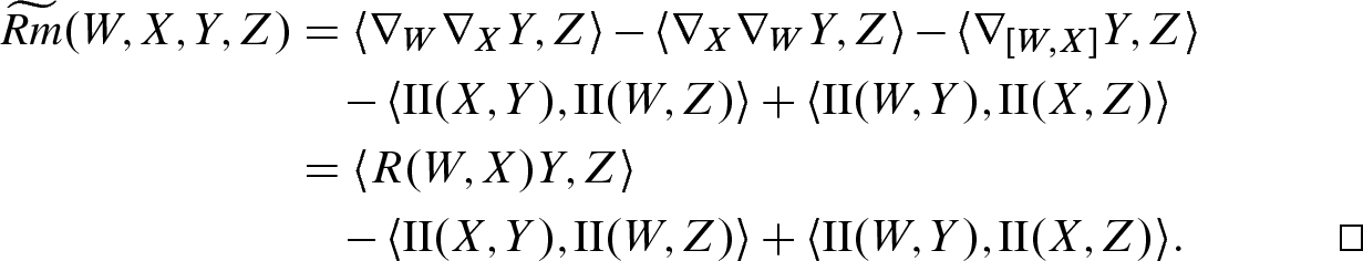
There is one other fundamental submanifold equation, which relates the normal part of the ambient curvature endomorphism to derivatives of the second fundamental form. We will not have need for it, but we include it here for completeness. To state it, we need to introduce a connection on the normal bundle of a Riemannian submanifold.

If (M, g) is a Riemannian submanifold of a Riemannian or pseudo-Riemannian manifold $\big ({{\widetilde{M}}},{\tilde{g}}\big )$ , the normal connection $\nabla ^\perp :\mathfrak X(M)\times \varGamma (NM) \mathrel {\rightarrow }\varGamma (NM)$ is defined by

$\begin{aligned} \nabla _X^\perp N = \big (\tilde{\nabla }_X N\big )^\perp , \end{aligned}$

where N is extended to a smooth vector field on a neighborhood of M in ${{\widetilde{M}}}$ .

Proposition 8.6.

If (M, g) is an embedded Riemannian submanifold of a Riemannian or pseudo-Riemannian manifold $\big ({{\widetilde{M}}},{\tilde{g}}\big )$ , then $\nabla ^\perp$ is a well-defined connection in NM, which is compatible with $\tilde{g}$ in the sense that for any two sections $$N_1,N_2$$

of NM and every $X\in \mathfrak X(M)$ , we have

$\begin{aligned} X\langle N_1,N_2\rangle = \big \langle \nabla _X^\perp N_1,N_2\big \rangle + \big \langle N_1,\nabla _X^\perp N_2\big \rangle . \end{aligned}$

$\blacktriangleright$ Exercise 8.7. Prove the preceding proposition.

We need the normal connection primarily to make sense of tangential covariant derivatives of the second fundamental form. To do so, we make the following definitions. Let $F\mathrel {\rightarrow }M$ denote the bundle whose fiber at each point $p\in M$ is the set of bilinear maps $T_pM\times T_pM\mathrel {\rightarrow }N_pM$ . It is easy to check that F is a smooth vector bundle over M, and that smooth sections of F correspond to smooth maps $\mathfrak X(M)\times \mathfrak X(M)\mathrel {\rightarrow }\varGamma (NM)$ that are bilinear over $C^\infty (M)$ , such as the second fundamental form. Define a connection $\nabla ^F$ in F as follows: if B is any smooth section of F, let $\nabla ^F_XB$ be the smooth section of F defined by

$\begin{aligned} \big (\nabla ^F_X B\big )(Y,Z) = \nabla _X^\perp ( B(Y, Z)) - B\big ( \nabla _X Y,\ Z\big ) - B\big ( Y,\ \nabla _X Z\big ). \end{aligned}$

$\blacktriangleright$ Exercise 8.8. Prove that $\nabla ^F$ is a connection in F.

Now we are ready to state the last of the fundamental equations for submanifolds. This equation was independently discovered (in the special case of surfaces in $\mathbb {R}^3$ ) by Karl M. Peterson (1853), Gaspare Mainardi (1856), and Delfino Codazzi (1868–1869), and is sometimes designated by various combinations of these three names. For the sake of simplicity we use the traditional but historically inaccurate name Codazzi equation.

Theorem 8.9

(The Codazzi Equation). Suppose (M, g) is an embedded Riemannian submanifold of a Riemannian or pseudo-Riemannian manifold $\big ({{\widetilde{M}}},{\tilde{g}}\big )$ . For all $W,X, Y\in \mathfrak X(M)$ , the following equation holds:

$\begin{aligned} \big (\tilde{R}(W,X)Y\big )^\perp = \big (\nabla _W^F \mathrm {II}\big )(X,Y) - \big (\nabla _X^F\mathrm {II}\big )(W, Y). \end{aligned}$

(8.6)

Proof.

It suffices to show that both sides of (8.6) give the same result when we take their inner products with an arbitrary smooth normal vector field N along M:

$\begin{aligned} \big \langle \tilde{R}(W,X)Y,\ N\big \rangle = \big \langle \big (\nabla ^F_W\mathrm {II}\big )(X,Y),\ N\big \rangle - \big \langle \big (\nabla ^F_X\mathrm {II}\big )(W, Y),\ N\big \rangle . \end{aligned}$

(8.7)

We begin as in the proof of the Gauss equation: after extending the vector fields to a neighborhood of M and applying the Gauss formula, we obtain

$\begin{aligned} \widetilde{ Rm }(W,X,Y,N)&= \big <{\tilde{\nabla }}_W\big (\nabla _X Y+\mathrm {II}(X,Y)\big ) - {\tilde{\nabla }}_X\big (\nabla _W Y+\mathrm {II}(W,Y)\big ) \\&\qquad - {\tilde{\nabla }}_{[W, X]}Y,\ N\big \rangle . \end{aligned}$

Now when we expand the covariant derivatives, we need only pay attention to the normal components. This yields

$\begin{aligned} \widetilde{ Rm }&\left( W,X,Y,N\right) \\&= \big \langle \mathrm {II}\left( W,\nabla _X Y\right) +\left( \nabla ^F_W\mathrm {II}\right) \left( X,Y\right) + \mathrm {II}\left( \nabla _WX,Y\right) + \mathrm {II}\left( X,\nabla _W Y\right) ,\ N\big \rangle \\&\quad - \big \langle \mathrm {II}\left( X,\nabla _W Y\right) +\left( \nabla ^F_X\mathrm {II}\right) \left( W,Y\right) + \mathrm {II}\left( \nabla _XW,Y\right) + \mathrm {II}\left( W,\nabla _X Y\right) ,\ N\big \rangle \\&\quad -\big \langle \mathrm {II}\left( [W,X], Y\right) ,\ N\big \rangle . \end{aligned}$

The terms involving $\nabla _XY$ and $\nabla _WY$ cancel each other in pairs, and three other terms sum to zero because $\nabla _WX - \nabla _XW -[W, X]=0$ . What remains is (8.7). $\square$

Curvature of a Curve

By studying the curvatures of curves, we can give a more geometric interpretation of the second fundamental form. Suppose (M, g) is a Riemannian or pseudo-Riemannian manifold, and $\gamma :I\mathrel {\rightarrow }M$ is a smooth unit-speed curve in M. We define the (geodesic) curvature of ${\varvec{\gamma }}$ as the length of the acceleration vector field, which is the function $\kappa :I\mathrel {\rightarrow }\mathbb {R}$ given by

$\begin{aligned} \kappa (t) = \left| {D_t\gamma '(t)}\right| . \end{aligned}$

If $\gamma$ is an arbitrary regular curve in a Riemannian manifold (not necessarily of unit speed), we first find a unit-speed reparametrization $\tilde{\gamma }= \gamma \circ \varphi$ , and then define the curvature of $\gamma$ at t to be the curvature of $\tilde{\gamma }$ at $\varphi ^{-1}(t)$ . In a pseudo-Riemannian manifold, the same approach works, but we have to restrict the definition to curves $\gamma$ such that $|\gamma '(t)|$ is everywhere nonzero. Problem 8-6 gives a formula that can be used in the Riemannian case to compute the geodesic curvature directly without explicitly finding a unit-speed reparametrization.

From the definition, it follows that a smooth unit-speed curve has vanishing geodesic curvature if and only if it is a geodesic, so the geodesic curvature of a curve can be regarded as a quantitative measure of how far it deviates from being a geodesic. If $M=\mathbb {R}^n$ with the Euclidean metric, the geodesic curvature agrees with the notion of curvature introduced in advanced calculus courses.

Now suppose $\big ({{\widetilde{M}}},{\tilde{g}}\big )$ is a Riemannian or pseudo-Riemannian manifold and (M, g) is a Riemannian submanifold. Every regular curve $\gamma :I\mathrel {\rightarrow }M$ has two distinct geodesic curvatures: its intrinsic curvature $\kappa$ as a curve in M, and its extrinsic curvature $\tilde{\kappa }$ as a curve in ${{\widetilde{M}}}$ . The second fundamental form can be used to compute the relationship between the two.

Proposition 8.10

(Geometric Interpretation of $\varvec{\mathrm {II}}$ ). Suppose (M, g) is an embedded Riemannian submanifold of a Riemannian or pseudo-Riemannian manifold $\big ({{\widetilde{M}}},{\tilde{g}}\big )$ , $p\in M$ , and $v\in T_pM$ .

(a)
$\mathrm {II}(v, v)$ is the $\tilde{g}$ -acceleration at p of the g-geodesic $\gamma _v$ .
(b)
If v is a unit vector, then $\left| \mathrm {II}(v, v)\right|$ is the $\tilde{g}$ -curvature of $\gamma _v$ at p.

Proof.

Suppose $\gamma :(-\varepsilon ,\varepsilon )\mathrel {\rightarrow }M$ is any regular curve with $\gamma (0)=p$ and $\gamma '(0)=v$ . Applying the Gauss formula (Corollary 8.3) to the vector field $\gamma '$ along $\gamma$ , we obtain

$\begin{aligned} {\tilde{D}_t\gamma '} = {D_t\gamma '} + \mathrm {II}(\gamma ',\gamma '). \end{aligned}$

If $\gamma$ is a g-geodesic in M, this formula simplifies to

$\begin{aligned} {\tilde{D}_t\gamma '} = \mathrm {II}(\gamma ',\gamma '). \end{aligned}$

Both conclusions of the proposition follow from this. $\square$

Note that the second fundamental form is completely determined by its values of the form $\mathrm {II}(v, v)$ for unit vectors v, by the following lemma.

Lemma 8.11.

Suppose V is an inner product space, W is a vector space, and $B, B':V\times V\mathrel {\rightarrow }W$ are symmetric and bilinear. If $$B(v,v)=B'(v, v)$$ for every unit vector $v\in V$ , then $$B=B'$$ .

Proof.

Every vector $v\in V$ can be written $v=\lambda \hat{v}$ for some unit vector $\hat{v}$ , so the bilinearity of B and $$B'$$

implies

for every v, not just unit vectors. The result then follows from the following polarization identity, which is proved in exactly the same way as its counterpart (2.2) for inner products:

../images/56724_2_En_8_Chapter/56724_2_En_8_Equ112_HTML.png

Because the intrinsic and extrinsic accelerations of a curve are usually different, it is generally not the case that a $\tilde{g}$ -geodesic that starts tangent to M stays in M; just think of a sphere in Euclidean space, for example. A Riemannian submanifold (M, g) of $\big ({{\widetilde{M}}},{\tilde{g}}\big )$ is said to be totally geodesic if every ${\tilde{g}}$ -geodesic that is tangent to M at some time $$t_0$$ stays in M for all t in some interval $(t_0-\varepsilon , t_0+\varepsilon )$ .

Proposition 8.12.

Suppose (M, g) is an embedded Riemannian submanifold of a Riemannian or pseudo-Riemannian manifold $\big ({{\widetilde{M}}},{\tilde{g}}\big )$ , The following are equivalent:

(a)
M is totally geodesic in ${{\widetilde{M}}}$ .
(b)
Every g-geodesic in M is also a ${\tilde{g}}$ -geodesic in ${{\widetilde{M}}}$ .
(c)
The second fundamental form of M vanishes identically.

Proof.

We will prove (a) $\Rightarrow$ (b) $\Rightarrow$ (c) $\Rightarrow$ (a). First assume that M is totally geodesic. Let $\gamma :I\mathrel {\rightarrow }M$ be a g-geodesic. For each $t_0\in I$ , let $\tilde{\gamma }:\tilde{I}\mathrel {\rightarrow }{{\widetilde{M}}}$ be the $\tilde{g}$ -geodesic with $\tilde{\gamma }(t_0) = \gamma (t_0)$ and $\tilde{\gamma }'(t_0) = \gamma '(t_0)$ . The hypothesis implies that there is some open interval $$I_0$$

containing $$t_0$$

such that $\tilde{\gamma }(t)\in M$ for $t\in I_0$ . On $$I_0$$

, the Gauss formula (8.2) for $\tilde{\gamma }'$ reads

$\begin{aligned} 0 = \tilde{D}_t\tilde{\gamma }' = D_t\tilde{\gamma }' + \mathrm {II}\bigl (\tilde{\gamma }',\tilde{\gamma }'\bigr ). \end{aligned}$

Because the first term on the right is tangent to M and the second is normal, the two terms must vanish individually. In particular, $D_t\tilde{\gamma }'\equiv 0$ on $$I_0$$

, which means that $\tilde{\gamma }$ is also a g-geodesic there. By uniqueness of geodesics, therefore, $\gamma = \tilde{\gamma }$ on $$I_0$$

, so it follows in turn that $\gamma$ is a $\tilde{g}$ -geodesic there. Since the same is true in a neighborhood of every $t_0\in I$ , it follows that $\gamma$ is a $\tilde{g}$ -geodesic on its whole domain.

Next assume that every g-geodesic is a ${\tilde{g}}$ -geodesic. Let $p\in M$ and $v\in T_pM$ be arbitrary, and let $\gamma =\gamma _v:I\mathrel {\rightarrow }M$ be the g-geodesic with $\gamma (0)=p$ and $\gamma '(0)=v$ . The hypothesis implies that $\gamma$ is also a $\tilde{g}$ -geodesic. Thus $\tilde{D}_t\gamma ' = D_t\gamma '=0$ , so the Gauss formula yields $\mathrm {II}(\gamma ',\gamma ')=0$ along $\gamma$ . In particular, $\mathrm {II}(v, v)=0$ . By Lemma 8.11, this implies that $\mathrm {II}$ is identically zero.

Finally, assume that $\mathrm {II}\equiv 0$ , and let $\tilde{\gamma }:I\mathrel {\rightarrow }{{\widetilde{M}}}$ be a $\tilde{g}$ -geodesic such that $\tilde{\gamma }(t_0)\in M$ and $\tilde{\gamma }'(t_0)\in TM$ for some $t_0\in I$ . Let $\gamma :I\mathrel {\rightarrow }M$ be the g-geodesic with the same initial conditions: $\gamma (t_0)=\tilde{\gamma }(t_0)$ and $\gamma '(t_0)=\tilde{\gamma }'(t_0)$ . The Gauss formula together with the hypothesis $\mathrm {II}\equiv 0$ implies that $\tilde{D}_t\gamma = D_t\gamma = 0$ , so $\gamma$ is also a $\tilde{g}$ -geodesic. By uniqueness of geodesics, therefore, $\tilde{\gamma }=\gamma$ on the intersection of their domains, which implies that $\tilde{\gamma }(t)$ lies in M for t in some open interval around $$t_0$$ . $\square$

Hypersurfaces

Now we specialize the preceding considerations to the case in which M is a hypersurface (i.e., a submanifold of codimension 1) in ${{\widetilde{M}}}$ . Throughout this section, our default assumption is that (M, g) is an embedded n-dimensional Riemannian submanifold of an $$(n+1)$$ -dimensional Riemannian manifold $\bigl ({{\widetilde{M}}},\tilde{g}\bigr )$ . (The analogous formulas in the pseudo-Riemannian case are a little different; see Problem 8-19.)

In this situation, at each point of M there are exactly two unit normal vectors. In terms of any local adapted orthonormal frame $(E_1,\dots , E_{n+1})$ , the two choices are $\pm E_{n+1}$ . In a small enough neighborhood of each point of M, therefore, we can always choose a smooth unit normal vector field along M.

If both M and ${{\widetilde{M}}}$ are orientable, we can use an orientation to pick out a global smooth unit normal vector field along all of M. In general, though, this might or might not be possible. Since all of our computations in this chapter are local, we will always assume that we are working in a small enough neighborhood that a smooth unit normal field exists. We will address as we go along the question of how various quantities depend on the choice of normal vector field.

The Scalar Second Fundamental Form and the Shape Operator

Having chosen a distinguished smooth unit normal vector field N on the hypersurface $M\subseteq {{\widetilde{M}}}$ , we can replace the vector-valued second fundamental form $\mathrm {II}$ by a simpler scalar-valued form. The scalar second fundamental form of ${\varvec{M}}$ is the symmetric covariant 2-tensor field $h\in \varGamma \big (\Sigma ^2 T^*M\big )$ defined by $h = \mathrm {II}_N$ (see (8.3)); in other words,

$\begin{aligned} h(X,Y) = \langle N,\mathrm {II}(X, Y)\rangle . \end{aligned}$

(8.8)

Using the Gauss formula ${\tilde{\nabla }}_X Y = \nabla _X Y + \mathrm {II}(X, Y)$ and noting that $\nabla _X Y$ is orthogonal to N, we can rewrite the definition as

$\begin{aligned} h(X, Y) = \big \langle N,{\tilde{\nabla }}_X Y\big \rangle . \end{aligned}$

(8.9)

Also, since N is a unit vector spanning $$N{ M}$$

at each point, the definition of h is equivalent to

$\begin{aligned} \mathrm {II}(X,Y) = h(X, Y)N. \end{aligned}$

(8.10)

Note that replacing N by $$-N$$

multiplies h by $$-1$$

, so the sign of h depends on which unit normal is chosen; but h is otherwise independent of the choices.

The choice of unit normal field also determines a Weingarten map $W_N:\mathfrak X(M)\mathrel {\rightarrow }\mathfrak X(M)$ by (8.4); in the case of a hypersurface, we use the notation $$s= W_N$$

and call it the shape operator of $\varvec{M}$ . Alternatively, we can think of s as the (1, 1)-tensor field on M obtained from h by raising an index. It is characterized by

$\begin{aligned} \langle sX,Y\rangle = h(X,Y) \qquad \text {for all}~X, Y\in {\mathfrak {X}}(M). \end{aligned}$

Because h is symmetric, s is a self-adjoint endomorphism of TM, that is,

$\begin{aligned} \langle sX,Y\rangle = \langle X,sY\rangle \qquad \text {for all}~X, Y\in {\mathfrak {X}}(M). \end{aligned}$

As with h, the sign of s depends on the choice of N.

In terms of the tensor fields h and s, the formulas of the last section can be rewritten somewhat more simply. For this purpose, we will use two tensor operations defined in Chapter 7: the Kulkarni–Nomizu product of symmetric 2-tensors h, k is

../images/56724_2_En_8_Chapter/56724_2_En_8_Equ113_HTML.png

and the exterior covariant derivative of a smooth symmetric 2-tensor field T is

$\begin{aligned} (DT)(x,y,z) = -(\nabla T)(x,y,z) + (\nabla T)(x,z, y). \end{aligned}$

Theorem 8.13

(Fundamental Equations for a Hypersurface). Suppose (M, g) is a Riemannian hypersurface in a Riemannian manifold $\bigl ({{\widetilde{M}}},\tilde{g}\bigr )$ , and N is a smooth unit normal vector field along M.

(a)
The Gauss Formula for a Hypersurface: If $X, Y\in \mathfrak X(M)$ are extended to an open subset of ${{\widetilde{M}}}$ , then
$\begin{aligned} \tilde{\nabla }_XY = \nabla _XY + h(X, Y)N. \end{aligned}$
(b)
The Gauss Formula for a Curve in a Hypersurface: If $\gamma :I\mathrel {\rightarrow }M$ is a smooth curve and $X:I\mathrel {\rightarrow }TM$ is a smooth vector field along $\gamma$ , then
$\begin{aligned} \tilde{D}_tX = {D_tX} + h(\gamma ', X)N. \end{aligned}$
(c)
The Weingarten Equation for a Hypersurface: For every $X\in \mathfrak X(M)$ ,
$\begin{aligned} \tilde{\nabla }_XN = -sX. \end{aligned}$

(8.11)
(d)
The Gauss Equation for a Hypersurface: For all $W,X,Y, Z\in \mathfrak {X}(M)$ ,
(e)
The Codazzi Equation for a Hypersurface: For all $W,X, Y\in \mathfrak X(M)$ ,

(8.12)

Proof.

Parts (a), (b), and (d) follow immediately from substituting (8.10) into the general versions of the Gauss formula and Gauss equation. To prove (c), note first that the general version of the Weingarten equation can be written $\big (\tilde{\nabla }_X N\big )^\top = -sX$ . Since $\big \langle {\tilde{\nabla }}_X N, N\big \rangle = \frac{1}{2} X\big (|N|^2\big )=0$ , it follows that $\tilde{\nabla }_X N$ is tangent to M, so (c) follows.

To prove the hypersurface Codazzi equation, note that the fact that N is a unit vector field implies

$\begin{aligned} 0 = X|N|^2_{{\tilde{g}}} = 2 \big \langle \nabla ^\perp _X N,\ N\big \rangle _{\tilde{g}}. \end{aligned}$

Since N spans the normal bundle, this implies that N is parallel with respect to the normal connection. Moreover,

$\begin{aligned} \big (\nabla ^F_W\mathrm {II}\big )(X,Y)&= \nabla ^\perp _W (\mathrm {II}(X,Y)) - \mathrm {II}(\nabla _W X, Y) - \mathrm {II}(X,\nabla _W Y)\\&= \nabla ^\perp _W (h(X,Y)N) - \mathrm {II}(\nabla _W X, Y) - \mathrm {II}(X,\nabla _W Y)\\&= \Big (W (h(X,Y)) - h(\nabla _W X, Y) - h(X,\nabla _W Y)\Big )N\\&= \nabla _W(h)(X, Y)N. \end{aligned}$

Inserting this into the general form (8.6) of the Codazzi equation and using the fact that $\nabla h$ is symmetric in its first two indices yields

$\begin{aligned} \widetilde{ Rm }(W,X,Y,N)&= \nabla _W (h)(X,Y) - \nabla _X (h)(W,Y)\\&= (\nabla h)(X,Y,W) - (\nabla h)(W,Y,X)\\&= (\nabla h)(Y,X,W) - (\nabla h)(Y,W, X), \end{aligned}$

which is equivalent to (8.12). $\square$

Principal Curvatures

At every point $p\in M$ , we have seen that the shape operator s is a self-adjoint linear endomorphism of the tangent space $$T_pM$$ . To analyze such an operator, we recall some linear-algebraic facts about self-adjoint endomorphisms.

Lemma 8.14.

Suppose V is a finite-dimensional inner product space and $s:V\mathrel {\rightarrow }V$ is a self-adjoint linear endomorphism. Let C denote the set of unit vectors in V. There is a vector $v_0\in C$ where the function $v\mapsto \langle sv, v\rangle$ achieves its maximum among elements of C, and every such vector is an eigenvector of s with eigenvalue $\lambda _0 = \langle sv_0,v_0\rangle$ .

$\blacktriangleright$ Exercise 8.15. Use the Lagrange multiplier rule (Prop. A.29) to prove this lemma.

Proposition 8.16

(Finite-Dimensional Spectral Theorem). Suppose V is a finite-dimensional inner product space and $s:V\mathrel {\rightarrow }V$ is a self-adjoint linear endomorphism. Then V has an orthonormal basis of s-eigenvectors, and all of the eigenvalues are real.

Proof.

The proof is by induction on $n=\dim V$ . The $$n=1$$ result is easy, so assume that the theorem holds for some $n\ge 1$ and suppose $\dim V = n+1$ . Lemma 8.14 shows that s has a unit eigenvector $$b_0$$ with a real eigenvalue $\lambda _0$ . Let $B\subseteq V$ be the span of $$b_0$$ . Since $s(B)\subseteq B$ , self-adjointness of s implies $s\big (B^\perp \big )\subseteq B^\perp$ . The inductive hypothesis applied to $s|_{B^\perp }$ implies that $B^\perp$ has an orthonormal basis $(b_1,\dots , b_n)$ of s-eigenvectors with real eigenvalues, and then $(b_0,b_1,\dots , b_n)$ is the desired basis of V. $\square$

Applying this proposition to the shape operator $s:T_pM\mathrel {\rightarrow }T_pM$ , we see that s has real eigenvalues $\kappa _1,\dots ,\kappa _{n}$ , and there is an orthonormal basis $(b_1,\dots , b_{n})$ for $$T_pM$$

consisting of s-eigenvectors, with $sb_i=\kappa _ib_i$ for each i (no summation). In this basis, both h and s are represented by diagonal matrices, and h has the expression

$\begin{aligned} h(v, w) = \kappa _1 v^1w^1 +\dots + \kappa _{n} v^{n}w^{n}. \end{aligned}$

The eigenvalues of s at a point $p\in M$ are called the principal curvatures of ${\varvec{M}}\,$ at ${\varvec{p}}$ , and the corresponding eigenspaces are called the principal directions. The principal curvatures all change sign if we reverse the normal vector, but the principal directions and principal curvatures are otherwise independent of the choice of coordinates or bases.

There are two combinations of the principal curvatures that play particularly important roles for hypersurfaces. The Gaussian curvature is defined as $K=\det (s)$ , and the mean curvature as $H = ({1}/{n}) {{\,\mathrm{tr}\,}}(s) = (1/n) {{\,\mathrm{tr}\,}}_g (h)$ . Since the determinant and trace of a linear endomorphism are basis-independent, these are well defined once a unit normal is chosen. In terms of the principal curvatures, they are

$\begin{aligned} K = \kappa _1\kappa _2\cdots \kappa _{n}, \qquad H = \frac{1}{n} (\kappa _1+\dots +\kappa _{n}), \end{aligned}$

as can be seen by expressing s in terms of an orthonormal basis of eigenvectors. If N is replaced by $$-N$$

, then H changes sign, while K is multiplied by $$(-1)^n$$

Computations in Semigeodesic Coordinates

Semigeodesic coordinates (Prop. 6.41) provide an extremely convenient tool for computing the invariants of hypersurfaces.

Let $\big ({{\widetilde{M}}},{\tilde{g}}\big )$ be an $$(n{+}1)$$

-dimensional Riemannian manifold, and let $\big (x^1,\dots ,x^n, v\big )$ be semigeodesic coordinates on an open subset $U\subseteq {{\widetilde{M}}}$ . (For example, they might be Fermi coordinates for the hypersurface $M_0 = v^{-1}(0)$ ; see Example 6.43.) For each real number a such that $v^{-1}(a)\ne \varnothing$ , the level set $M_a = v^{-1}(a)$ is a properly embedded hypersurface in U. Let $$g_a$$

denote the induced metric on $$M_a$$

. Corollary 6.42 shows that ${\tilde{g}}$ is given by

$\begin{aligned} {\tilde{g}} = dv^2 + \sum _{ \alpha ,\beta = 1}^{n} g_{ \alpha \beta }\big (x^1,\dots ,x^{n}, v\big )dx^ \alpha \, dx^\beta . \end{aligned}$

(8.13)

The restrictions of $\big (x^1,\dots , x^n)$ give smooth coordinates for each hypersurface $$M_a$$

, and in those coordinates the induced metric $$g_a$$

is given by $g_a = g_{ \alpha \beta }dx^ \alpha \, dx^\beta |_{v=a}$ . (Here we use the summation convention with Greek indices running from 1 to n.) The vector field $\partial _v = \partial _{n+1}$ restricts to a unit normal vector field along each hypersurface $$M_a$$

As the next proposition shows, semigeodesic coordinates give us a simple formula for the second fundamental forms of all of the submanifolds $$M_a$$ at once.

Proposition 8.17.

With notation as above, the components in $\big (x^1,\dots , x^{n}\big )$ -coordinates of the scalar second fundamental form, the shape operator, and the mean curvature of $$(M_a, g_a)$$

$({\textit{denoted by}}~h_a, s_a, {\textit{and}}~H_a,~{\textit{respectively}})$ with respect to the normal $N = \partial _v$ are given by

$\begin{aligned} (h_a)_{\alpha \beta }&= -\frac{1}{2} \partial _v g_{\alpha \beta }\Big |_{v=a},\\ (s_a)^{\alpha }_\beta&= -\frac{1}{2} g^{\alpha \gamma }\partial _v g_{\gamma \beta }\Big |_{v=a},\\ H_a&= -\frac{1}{2n} g^{\alpha \beta }\partial _v g_{\alpha \beta }\Big |_{v=a}. \end{aligned}$

Proof.

The normal component of $\tilde{\nabla }_{\partial _\alpha }\partial _\beta$ is $\tilde{\varGamma }_{\alpha \beta }^{n+1}\partial _{v}$ , which Corollary 6.42 shows is equal to $-\tfrac{1}{2} \partial _v g_{\alpha \beta }\partial _r$ (noting that the roles of g and $\hat{g}$ in that corollary are being played here by ${\tilde{g}}$ and $$g_a$$

, respectively). Equation (8.9) evaluated at points of $$M_a$$

gives

$\begin{aligned} (h_a)_{\alpha \beta } = \big \langle \tilde{\nabla }_{\partial _\alpha }\partial _\beta , N\big \rangle _{{\tilde{g}}} = \big \langle -\tfrac{1}{2} \partial _v g_{\alpha \beta }\partial _v, \partial _v\big \rangle _{{\tilde{g}}} = -\tfrac{1}{2} \partial _v g_{\alpha \beta }. \end{aligned}$

The formulas for $$s_a$$

and

follow by using $(g^{\alpha \gamma })$ (the inverse matrix of $(g_{\alpha \gamma })$ ) to raise an index and then taking the trace. $\square$

Minimal Hypersurfaces

A natural question that has received a great deal of attention over the past century is this: Given a simple closed curve C in $\mathbb {R}^3$ , is there an embedded or immersed surface M with $\partial M = C$ that has least area among all surfaces with the same boundary? If so, what is it? Such surfaces are models of the soap films that are produced when a closed loop of wire is dipped in soapy water.

More generally, we can consider the analogous question for hypersurfaces in Riemannian manifolds. Suppose M is a compact codimension-1 submanifold with nonempty boundary in an $$(n+1)$$ -dimensional Riemannian manifold $\big ({{\widetilde{M}}},{\tilde{g}}\big )$ . By analogy with the case of surfaces in $\mathbb {R}^3$ , it is traditional to use the term area to refer to the n-dimensional volume of M with its induced Riemannian metric, and to say that M is area-minimizing if it has the smallest area among all compact embedded hypersurfaces in ${{\widetilde{M}}}$ with the same boundary. One key observation is the following theorem, which is an analogue for hypersurfaces of Theorem 6.4 about length-minimizing curves.

Theorem 8.18.

Let M be a compact codimension-1 submanifold with nonempty boundary in an $$(n+1)$$ -dimensional Riemannian manifold $\big ({{\widetilde{M}}},{\tilde{g}}\big )$ . If M is area-minimizing, then its mean curvature is identically zero.

Proof.

Let g denote the induced metric on M. The fact that M minimizes area among hypersurfaces with the same boundary means, in particular, that it minimizes area among small perturbations of M in a neighborhood of a single point. We will exploit this idea to prove that M must have zero mean curvature everywhere.

Let $p\in \mathrm{Int}\, M$ be arbitrary, let $\big (x^1,\dots ,x^{n}, v\big )$ be Fermi coordinates for M on an open set ${\smash [t]{\tilde{U}}}\subseteq {{\widetilde{M}}}$ containing p (see Example 6.43), and let $U = {\smash [t]{\tilde{U}}}\cap M$ . By taking ${\smash [t]{\tilde{U}}}$ sufficiently small, we can arrange that U is a regular coordinate ball in M (see p. 374) and ${\smash [t]{\tilde{U}}}\cap \partial M=\varnothing$ . We use $\big (x^1,\dots , x^n\big )$ as coordinates on M, and observe the summation convention with Greek indices running from 1 to n.

../images/56724_2_En_8_Chapter/56724_2_En_8_Fig2_HTML.png — Fig. 8.2:
The hypersurface

Let $\varphi$ be an arbitrary smooth real-valued function on M with compact support in U. For sufficiently small t, define a set $M_t\subseteq {{\widetilde{M}}}$ by

../images/56724_2_En_8_Chapter/56724_2_En_8_Equ115_HTML.png

(See Fig. 8.2.) Then $$M_t$$

is an embedded smooth hypersurface in ${{\widetilde{M}}}$ , which agrees with M outside of U and which coincides with the graph of $v=t\varphi$ in ${\smash [t]{\tilde{U}}}$ . Let $f_t:U\mathrel {\rightarrow }{\smash [t]{\tilde{U}}}$ be the graph parametrization of $M_t\cap {\smash [t]{\tilde{U}}}$ , given in Fermi coordinates by

$\begin{aligned} f_t\big (x^1,\dots , x^n\big ) = \big (x^1,\dots ,x^n, t\varphi (x)\big ). \end{aligned}$

(8.14)

Using this map, for each t we can define a diffeomorphism $F_t:M\mathrel {\rightarrow }M_t$ by

../images/56724_2_En_8_Chapter/56724_2_En_8_Equ116_HTML.png

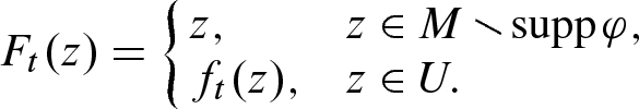
For each t, let $\hat{g}_t = \iota _{M_t}^*{\tilde{g}}$ denote the induced Riemannian metric on $$M_t$$

, and let $g_t=F_t^*\hat{g}_t=F_t^*{\tilde{g}}$ denote the pulled-back metric on M. When $$t=0$$

, we have

, and both $$g_0$$

and $\hat{g}_0$ are equal to the induced metric g on M. Since ${\tilde{g}}$ is given by (8.13) in Fermi coordinates, a simple computation shows that in U, $g_t = F_t^*{\tilde{g}}$ has the coordinate expression $g_t = (g_t)_{\alpha \beta }\, dx^\alpha \, dx^\beta$ , where

$\begin{aligned} (g_t)_{\alpha \beta } = t^2 \frac{\partial \varphi }{\partial x^\alpha } (x)\, \frac{\partial \varphi }{\partial x^\beta } (x) + g_{\alpha \beta }\big (x, t\varphi (x)\big ), \end{aligned}$

(8.15)

while on

../images/56724_2_En_8_Chapter/56724_2_En_8_IEq416_HTML.gif

is equal to g and thus is independent of t.

Since each $$M_t$$

is a smooth hypersurface with the same boundary as M, our hypothesis guarantees that $\mathrm{Area}\,(M_t,\hat{g}_t)$ achieves a minimum at $$t=0$$

. Because

is an isometry from $$(M, g_t)$$

to $(M_t,\hat{g}_t)$ , we can express this area as follows:

../images/56724_2_En_8_Chapter/56724_2_En_8_Equ117_HTML.png

The first term on the right is independent of t, and we can compute the second term explicitly in coordinates $\big (x^1,\dots , x^n\big )$ on U:

$\begin{aligned} \mathrm{Area}\,(U, g_t) = \int _{U} \sqrt{\det g_t}\, dx^1\cdots dx^n, \end{aligned}$

where $\det g_t$ denotes the determinant of the matrix $\big ((g_t)_{\alpha \beta }\big )$ defined by (8.15). The integrand above is a smooth function of t and $\big (x^1,\dots , x^n\big )$ , so the area is a smooth function of t. We have

$\begin{aligned} \begin{aligned} \left. \frac{d}{dt}\right| _{t=0} \mathrm{Area}\,(M_t,\hat{g}_t)&= \int _U \left. \frac{\partial }{\partial t} \right| _{t=0}\sqrt{\det g_t}\, dx^1\cdots dx^n\\&= \int _U \frac{1}{2} (\det g)^{-1/2}\left. \frac{\partial }{\partial t} \right| _{t=0}(\det g_t)\, dx^1\cdots dx^n. \end{aligned} \end{aligned}$

(8.16)

(The differentiation under the integral sign is justified because the integrand is smooth and has compact support in U.)

To compute the derivative of the determinant, note that the expansion by minors along, say, row $\alpha$ shows that the partial derivative of $\det$ with respect to the matrix entry in position $(\alpha ,\beta )$ is equal to the cofactor $\mathrm {cof\,}^{\alpha \beta }$ , and thus by the chain rule,

$\begin{aligned} \left. \frac{\partial }{\partial t} \right| _{t=0}(\det g_t) = \mathrm {cof\,}^{\alpha \beta } \left. \frac{\partial }{\partial t} \right| _{t=0}(g_t)_{\alpha \beta }. \end{aligned}$

(8.17)

On the other hand, Cramer’s rule shows that the $(\alpha ,\beta )$ component of the inverse matrix is given by $g^{\alpha \beta } = (\det g)^{-1}\mathrm {cof\,}^{\alpha \beta }$ . Thus from (8.17) and (8.15) we obtain

$\begin{aligned} \left. \frac{\partial }{\partial t} \right| _{t=0}(\det g_t) =(\det g)g^{\alpha \beta } \left. \frac{\partial }{\partial t} \right| _{t=0} (g_t)_{\alpha \beta } = (\det g) g^{\alpha \beta } \frac{\partial g_{\alpha \beta }}{\partial v}\varphi . \end{aligned}$

Inserting this into (8.16) and using the result of Proposition 8.17, we conclude that

$\begin{aligned} \begin{aligned} \left. \frac{d}{dt}\right| _{t=0} \mathrm{Area}\,(M_t,\hat{g}_t)&= \int _U \frac{1}{2} (\det g)^{1/2}g^{\alpha \beta } \frac{\partial g_{\alpha \beta }}{\partial v}\varphi \, dx^1\cdots dx^n\\&= -n \int _U H\varphi \, dV_g, \end{aligned} \end{aligned}$

(8.18)

where H is the mean curvature of (M, g). Since $\mathrm{Area}\,(M_t,\hat{g}_t)$ attains a minimum at $$t=0$$

, we conclude that $\int _U H\varphi \, dV_g=0$ for every such $\varphi$ .

Now suppose for the sake of contradiction that $H(p)\,{\ne }\, 0$ . If $$H(p){>} 0$$ , we can let $\varphi$ be a smooth nonnegative bump function that is positive at p and supported in a small neighborhood of p on which $$H>0$$ . The argument above shows that $\int _U H\varphi \, dV_g=0$ , which is impossible because the integrand is nonnegative on U and positive on an open set. A similar argument rules out $$H(p)<0$$ . Since p was an arbitrary point in $\mathrm{Int}\, M$ , we conclude that $H\equiv 0$ on $\mathrm{Int}\, M$ , and then by continuity on all of M. $\square$

Because of the result of Theorem 8.18, a hypersurface (immersed or embedded, with or without boundary) that has mean curvature identically equal to zero is called a minimal hypersurface (or a minimal surface when it has dimension 2). It is an unfortunate historical accident that the term “minimal hypersurface” is defined in this way, because in fact, a minimal hypersurface is just a critical point for the area, not necessarily area-minimizing. It can be shown that as in the case of geodesics, a small enough piece of every minimal hypersurface is area-minimizing.

As a complement to the above theorem about hypersurfaces that minimize area with fixed boundary, we have the following result about hypersurfaces that minimize area while enclosing a fixed volume.

Theorem 8.19.

Suppose $\big ({{\widetilde{M}}}, g\big )$ is a Riemannian $$(n+1)$$ -manifold, $D\subseteq {{\widetilde{M}}}$ is a compact regular domain, and $M=\partial D$ . If M has the smallest surface area among boundaries of compact regular domains with the same volume as D, then M has constant mean curvature (computed with respect to the outward unit normal).

Proof.

Let g denote the induced metric on M. Assume for the sake of contradiction that the mean curvature H of M is not constant, and let $p, q\in M$ be points such that $$H(p)<H(q)$$ .

Since M is compact, it has an $\varepsilon$ -tubular neighborhood for some $\varepsilon >0$ by Theorem 5.25. As in the previous proof, let $\big (x^1,\dots ,x^{n}, v\big )$ be Fermi coordinates for M on an open set ${\smash [t]{\tilde{U}}}\subseteq {{\widetilde{M}}}$ containing p, and let $U = {\smash [t]{\tilde{U}}}\cap M$ . We may assume that U is a regular coordinate ball in M and the image of the chart is a set of the form $\hat{U}\times (-\varepsilon ,\varepsilon )$ for some open subset $\hat{U}\subseteq \mathbb {R}^n$ . Similarly, let $\big (y^1,\dots ,y^{n}, w\big )$ be Fermi coordinates for M on an open set ${\smash [t]{\widetilde{W}}}\subseteq {{\widetilde{M}}}$ containing q and satisfying the analogous conditions, and let $W = {\smash [t]{\widetilde{W}}}\cap M$ . By replacing v with its negative if necessary, we can arrange that $D\cap {\smash [t]{\tilde{U}}}$ is the set where $v\le 0$ , and similarly for w. Also, by shrinking both domains, we can assume that the mean curvature of M satisfies $H\le H_1$ on U and $H\ge H_2$ on W, where $$H_1,H_2$$ are constants such that $$H(p)<H_1<H_2<H(q)$$ .

Let $\varphi$ and $\psi$ be smooth real-valued functions on M, with $\varphi$ compactly supported in U and $\psi$ compactly supported in W, and satisfying $\int _U \varphi \,dV_g = \int _W \psi \, dV_g = 1$ . For sufficiently small $s, t\in \mathbb {R}$ , define a subset $D_{s, t}\subseteq \widetilde{M}$ as follows:

../images/56724_2_En_8_Chapter/56724_2_En_8_Equ118_HTML.png

and let $M_{s,t} = \partial D_{s, t}$ , so $D_{0,0}=D$ and $M_{0,0} = M$ (see Fig. 8.3). For sufficiently small s and t, the set $D_{s, t}$ is a regular domain and $M_{s, t}$ is a compact smooth hypersurface, and $\mathrm{Vol}(D_{s, t})$ and $\mathrm{Area}\,(M_{s, t})$ are both smooth functions of (s, t). For convenience, write $V(s,t) = \mathrm{Vol}(D_{s, t})$ and $A(s,t)=\mathrm{Area}\,(M_{s, t})$ .

../images/56724_2_En_8_Chapter/56724_2_En_8_Fig3_HTML.png — Fig. 8.3:
The domain $D_{s, t}$

$$D_{s, t}$$ — Fig. 8.3:
The domain $D_{s, t}$

The same argument that led to (8.18) shows that

$\begin{aligned} \frac{\partial A}{\partial s}(0,0) = -n \int _U H\varphi \, dV_g, \qquad \frac{\partial A}{\partial t}(0,0) = -n \int _W H\psi \, dV_g. \end{aligned}$

To compute the partial derivatives of the volume, we just note that if we hold $$t=0$$

fixed and let s vary, the only change in volume occurs in the part of $D_{s, t}$ contained in ${\smash [t]{\tilde{U}}}$ , so the fundamental theorem of calculus gives

$\begin{aligned} \frac{\partial V}{\partial s}(0,0)&= \left. \frac{d}{d s}\right| _{s=0}\mathrm{Vol}\big (D_{s, 0}\cap {\smash [t]{\tilde{U}}}\big )\\&= \left. \frac{d}{d s}\right| _{s=0}\int _{U}\left( \int _{-\varepsilon }^{s\varphi (x)}\sqrt{\det {\tilde{g}}(x,v)}\, dv\right) dx^1\cdots dx^n\\&= \int _{U}\left( \left. \frac{d}{d s}\right| _{s=0}\int _{-\varepsilon }^{s\varphi (x)}\sqrt{\det {\tilde{g}}(x,v)}\, dv\right) dx^1\cdots dx^n\\&= \int _{U} \varphi (x) \sqrt{\det {\tilde{g}}(x, 0)}\, dx^1\cdots dx^n = \int _U \varphi \, dV_g =1, \end{aligned}$

where the differentiation under the integral sign in the third line is justified just like (8.16), and in the last line we used the fact that $g_{\alpha \beta }(x) = {\tilde{g}}_{\alpha \beta }(x, 0)$ in these coordinates. Similarly, $\partial V/\partial t(0,0)=1$ .

Because $V(0,0) = \mathrm{Vol}(D)$ and $\partial V/\partial t(0,0)\ne 0$ , the implicit function theorem guarantees that there is a smooth function $\lambda :(-\delta ,\delta )\mathrel {\rightarrow }\mathbb {R}$ for some $\delta >0$ such that $V(s,\lambda (s))\equiv \mathrm{Vol}(D)$ . The chain rule then implies

$\begin{aligned} 0 = \left. \frac{d}{d s}\right| _{s=0} V(s,\lambda (s)) = \frac{\partial V}{\partial s}(0,0) + \lambda '(0) \frac{\partial V}{\partial t}(0,0) = 1 + \lambda '(0). \end{aligned}$

Thus $\lambda '(0) = -1$ .

Our hypothesis that M minimizes area implies that

$\begin{aligned} 0&= \left. \frac{d}{d s}\right| _{s=0} A(s,\lambda (s)) = \frac{\partial A}{\partial s}(0,0) + \lambda '(0) \frac{\partial A}{\partial t}(0,0) \\&= -n \int _U H\varphi \, dV_g + n\int _W H\psi \, dV_g, \end{aligned}$

and thus $\int _U H\varphi \, dV_g = \int _W H\psi \, dV_g$ . But our choice of U and V together with the fact that $\int _U \varphi \,dV_g = \int _W \psi \, dV_g = 1$ guarantees that $\int _U H\varphi \, dV_g \le H_1< H_2 \le \int _W H\psi \, dV_g$ , which is a contradiction. $\square$

We do not pursue minimal or constant-mean-curvature hypersurfaces any further in this book, but you can find a good introductory treatment in [CM11].

Hypersurfaces in Euclidean Space

Now we specialize even further, to hypersurfaces in Euclidean space. In this section, we assume that $M\subseteq \mathbb {R}^{n+1}$ is an embedded n-dimensional submanifold with the induced Riemannian metric. The Euclidean metric will be denoted as usual by ${\bar{g}}$ , and covariant derivatives and curvatures associated with ${\bar{g}}$ will be indicated by a bar. The induced metric on M will be denoted by g.

In this setting, because $\overline{ Rm }\equiv 0$ , the Gauss and Codazzi equations take even simpler forms:

../images/56724_2_En_8_Chapter/56724_2_En_8_Equ19_HTML.png

(8.19)

../images/56724_2_En_8_Chapter/56724_2_En_8_Equ20_HTML.png

(8.20)

or in terms of a local frame for M,

$\begin{aligned} h_{il}h_{jk} - h_{ik}h_{jl}&= R_{ijkl} ,\end{aligned}$

(8.21)

$\begin{aligned} h_{ij;k} - h_{ik;j}&= 0. \end{aligned}$

(8.22)

In particular, this means that the Riemann curvature tensor of a hypersurface in $\mathbb {R}^{n+1}$ is completely determined by the second fundamental form. A symmetric 2-tensor field that satisfies $$Dh=0$$

is called a Codazzi tensor, so (8.20) can be expressed succinctly by saying that h is a Codazzi tensor.

$\blacktriangleright$ Exercise 8.20. Show that a smooth 2-tensor field h on a Riemannian manifold is a Codazzi tensor if and only if both h and $\nabla h$ are symmetric.

The equations (8.19)–(8.20) can be viewed as compatibility conditions for the existence of an embedding or immersion into Euclidean space with prescribed first and second fundamental forms. If (M, g) is a Riemannian n-manifold and h is a given smooth symmetric 2-tensor field on M, then Theorem 8.13 shows that these two equations are necessary conditions for the existence of an isometric immersion $M\mathrel {\rightarrow }\mathbb {R}^{n+1}$ for which h is the scalar second fundamental form. (Note that an immersion is locally an embedding, so the theorem applies in a neighborhood of each point.) It is a remarkable fact that the Gauss and Codazzi equations are actually sufficient, at least locally. A sketch of a proof of this fact, called the fundamental theorem of hypersurface theory, can be found in [Pet16, pp. 108–109].

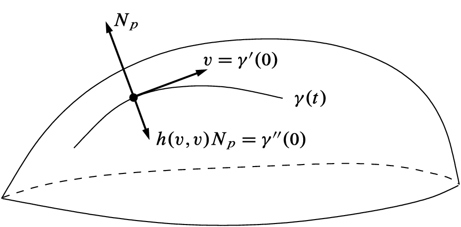
../images/56724_2_En_8_Chapter/56724_2_En_8_Fig4_HTML.png — Fig. 8.4:
Geometric interpretation of h(v, v)

In the setting of a hypersurface $M\subseteq \mathbb {R}^{n+1}$ , we can give some very concrete geometric interpretations of the quantities we have defined so far. We begin with curves. For every unit vector $v\in T_pM$ , let $\gamma =\gamma _v:I\mathrel {\rightarrow }M$ be the g-geodesic in M with initial velocity v. Then the Gauss formula shows that the ordinary Euclidean acceleration of $\gamma$ at 0 is $\gamma ''(0) = \bar{D}_t\gamma '(0) = h(v, v)N_p$ (Fig. 8.4). Thus |h(v, v)| is the Euclidean curvature of $\gamma$ at 0, and $h(v, v) = \langle \gamma ''(0), N_p\rangle >0$ if and only if $\gamma ''(0)$ points in the same direction as $$N_p$$ . In other words, h(v, v) is positive if $\gamma$ is curving in the direction of $$N_p$$ , and negative if it is curving away from $$N_p$$ .

The next proposition shows that this Euclidean curvature can be interpreted in terms of the radius of the “best circular approximation,” as mentioned in Chapter 1.

Proposition 8.21.

Suppose $\gamma :I\mathrel {\rightarrow }\mathbb {R}^m$ is a unit-speed curve, $t_0\in I$ , and $\kappa (t_0)\ne 0$ .

(a)
There is a unique unit-speed parametrized circle $c:\mathbb {R}\mathrel {\rightarrow }\mathbb {R}^m$ , called the osculating circle at ${\varvec{\gamma (t}}_{\varvec{0)}}$ , with the property that c and $\gamma$ have the same position, velocity, and acceleration at .
(b)
The Euclidean curvature of $\gamma$ at is $\kappa (t_0)=1/R$ , where R is the radius of the osculating circle.

Proof.

An easy geometric argument shows that every circle in $\mathbb {R}^m$ with center q and radius R has a unit-speed parametrization of the form

$\begin{aligned} c(t) = q + R\,\cos \Big (\frac{t-t_0}{R}\Big )v + R\,\sin \Big (\frac{t-t_0}{R}\Big )w, \end{aligned}$

where (v, w) is a pair of orthonormal vectors in $\mathbb {R}^m$ . By direct computation, such a parametrization satisfies

$\begin{aligned} c(t_0) = q + Rv,\qquad c'(t_0) = w,\qquad c''(t_0) = -\frac{1}{R}v. \end{aligned}$

Thus if we put

$\begin{aligned} R = \frac{1}{|\gamma ''(t_0)|} = \frac{1}{\kappa (t_0)},\quad v = -R\gamma ''(t_0),\quad w = \gamma '(t_0),\quad q = \gamma (t_0) - Rv, \end{aligned}$

we obtain a circle satisfying the required conditions, and its radius is equal to $1/\kappa (t_0)$ by construction. Uniqueness is left as an exercise. $\square$

$\blacktriangleright$ Exercise 8.22. Complete the proof of the preceding proposition by proving uniqueness of the osculating circle.

Computations in Euclidean Space

When we wish to compute the invariants of a Euclidean hypersurface $M\subseteq \mathbb {R}^{n+1}$ , it is usually unnecessary to go to all the trouble of computing Christoffel symbols. Instead, it is usually more effective to use either a defining function or a parametrization to compute the scalar second fundamental form, and then use (8.21) to compute the curvature. Here we describe several contexts in which this computation is not too hard.

Usually the computations are simplest if the hypersurface is presented in terms of a local parametrization. Suppose $M\subseteq \mathbb {R}^{n+1}$ is a smooth embedded hypersurface, and let $X:U \mathrel {\rightarrow }\mathbb {R}^{n+1}$ be a smooth local parametrization of M. The coordinates $\left( u^1,\dots , u^n\right)$ on $U\subseteq \mathbb {R}^n$ thus give local coordinates for M. The coordinate vector fields $\partial _i = \partial /\partial u^i$ push forward to vector fields $dX\left( \partial _i\right)$ on M, which we can view as sections of the restricted tangent bundle $T\mathbb {R}^{n+1}|_{M}$ , or equivalently as $\mathbb {R}^{n+1}$ -valued functions. If we think of $X(u) = \left( X^1(u),\dots , X^{n+1}(u)\right)$ as a vector-valued function of u, these vectors can be written as

$\begin{aligned} dX_u\left( \partial _i\right) = \partial _i X(u) = \big (\partial _i X^1(u),\dots ,\partial _i X^{n+1}(u)\big ). \end{aligned}$

For simplicity, write $X_i = \partial _i X$ .

Once these vector fields are computed, a unit normal field can be computed as follows: Choose any coordinate vector field $\partial /\partial x^{j_0}$ that is not contained in $\mathrm{span}\left( X_1,\dots , X_n\right)$ (there will always be one, at least in a neighborhood of each point). Then apply the Gram–Schmidt algorithm to the local frame $\big (X_1,\dots , X_n,\partial /\partial x^{j_0}\big )$ along M to obtain an adapted orthonormal frame $\left( E_1,\dots , E_{n+1}\right)$ . The two choices of unit normal are $N = \pm E_{n+1}$ .

The next proposition gives a formula for the second fundamental form that is often easy to use for computation.

Proposition 8.23.

Suppose $M\subseteq \mathbb {R}^{n+1}$ is an embedded hypersurface, $X:U\mathrel {\rightarrow }M$ is a smooth local parametrization of M, $\left( X_1,\dots , X_n\right)$ is the local frame for TM determined by X, and N is a unit normal field on M. Then the scalar second fundamental form is given by

$\begin{aligned} h\left( X_i, X_j\right) = \left\langle \frac{\partial ^2 X}{\partial u^i \partial u^j}, N\right\rangle . \end{aligned}$

(8.23)

Proof.

Let $u_0=\left( u_0^1,\dots , u_0^n\right)$ be an arbitrary point of U and let $p = X(u_0)\in M$ . For each $i\in \{1,\dots , n\}$ , the curve $\gamma (t) = X\left( u_0^1,\dots , u_0^i+t,\dots , u_0^n\right)$ is a smooth curve in M whose initial velocity is $$X_i$$

. Regarding the normal field N as a smooth map from M to $\mathbb {R}^{n+1}$ , we have

$\begin{aligned} \frac{\partial }{\partial u^i}N(X(u_0)) = (N\circ \gamma )'(0) = \bar{\nabla }_{X_i}N(X(u_0)). \end{aligned}$

Because $X_j = \partial X/\partial u^j$ is tangent to M and N is normal, the following expression is zero for all $u\in U$ :

$\begin{aligned} \left\langle \frac{\partial X}{\partial u^j}(u), N(X(u))\right\rangle . \end{aligned}$

Differentiating with respect to $$u^i$$

and using the product rule for ordinary inner products in $\mathbb {R}^{n+1}$ yields

$\begin{aligned} 0&= \left\langle \frac{\partial ^2 X}{\partial u^i\partial u^j}(u), N(X(u))\right\rangle + \left\langle \frac{\partial X}{\partial u^j}(u), \bar{\nabla }_{X_i(u)}N(X(u))\right\rangle . \end{aligned}$

By the Weingarten equation (8.11), the last term on the right becomes

$\begin{aligned} \left\langle X_j(u), -s(X_i(u))\right\rangle = - h(X_j(u), X_i(u)). \end{aligned}$

Inserting this above yields (8.23). $\square$

Here is an application of this formula: it shows how the principal curvatures give a concise description of the local shape of an embedded hypersurface by approximating the surface with the graph of a quadratic function.

Proposition 8.24.

Suppose $M\subseteq \mathbb {R}^{n+1}$ is a Riemannian hypersurface. Let $p\in M$ , and let $\kappa _1,\dots ,\kappa _{n}$ denote the principal curvatures of M at p with respect to some choice of unit normal. Then there is an isometry $\varphi :\mathbb {R}^{n+1}\mathrel {\rightarrow }\mathbb {R}^{n+1}$ that takes p to the origin and takes a neighborhood of p in M to a graph of the form $x^{n+1} = f(x^1,\dots , x^n)$ , where

$\begin{aligned} f(x) = \frac{1}{2} \big (\kappa _1 (x^1)^2 + \dots + \kappa _{n} (x^{n})^2\big ) + O\big (|x|^3\big ). \end{aligned}$

(8.24)

Proof.

Replacing M by its image under a translation and a rotation (which are Euclidean isometries), we may assume that p is the origin and $$T_pM$$ is equal to the span of $(\partial _1,\dots ,\partial _n)$ . Then after reflecting in the $\big (x^1,\dots , x^n\big )$ -hyperplane if necessary, we may assume that the chosen unit normal is $(0,\dots , 0,1)$ . By an orthogonal transformation in the first n variables, we can also arrange that the scalar second fundamental form at 0 is diagonal with respect to the basis $(\partial _1,\dots ,\partial _n)$ , with diagonal entries $(\kappa _1,\dots ,\kappa _n)$ .

It follows from the implicit function theorem that there is some neighborhood U of 0 such that $M\cap U$ is the graph of a smooth function of the form $x^{n+1} = f\left( x^1,\dots , x^n\right)$ with $$f(0)=0$$

. A smooth local parametrization of M is then given by $X(u) = \left( u^1,\dots ,u^n, f(u)\right)$ , and the fact that $$T_0M$$

is spanned by $\big (\partial /\partial x^1,\dots , \partial /\partial x^n\big )$ guarantees that $\partial _1f(0) = \dots = \partial _nf(0)=0$ . Because $X_i = \partial /\partial x^i$ at 0, Proposition 8.23 then yields

$\begin{aligned} h\left( \frac{\partial }{\partial x^i},\frac{\partial }{\partial x^j}\right) = \left\langle \left( 0,\dots , 0,\frac{\partial ^2 f}{\partial x^i\partial x^j}(0)\right) , (0,\dots , 0,1)\right\rangle = \frac{\partial ^2 f}{\partial x^i\partial x^j}(0). \end{aligned}$

It follows from our normalization that the matrix of second derivatives of f at 0 is diagonal, and its diagonal entries are the principal curvatures of M at that point. Then (8.24) follows from Taylor’s theorem. $\square$

Here is another approach. When it is practical to write down a smooth vector field $N = N^i\partial _i$ on an open subset of $\mathbb {R}^{n+1}$ that restricts to a unit normal vector field along M, then the shape operator can be computed straightforwardly using the Weingarten equation and observing that the Euclidean covariant derivatives of N are just ordinary directional derivatives in Euclidean space. Thus for every vector $X=X^j\partial _j$ tangent to M, we have

$\begin{aligned} sX = - \bar{\nabla }_X N = -\sum _{i, j=1}^{n+1}X^j(\partial _j N^i)\partial _i. \end{aligned}$

(8.25)

One common way to produce such a smooth vector field is to work with a local defining function for M: Recall that this is a smooth real-valued function defined on some open subset $U\subseteq \mathbb {R}^{n+1}$ such that $U\cap M$ is a regular level set of F (see Prop. A.27). The definition ensures that ${{\,\mathrm{grad}\,}}F$ (the gradient of F with respect to $\bar{g}$ ) is nonzero on some neighborhood of $M\cap U$ , so a convenient choice for a unit normal vector field along M is

$\begin{aligned} N = \frac{{{\,\mathrm{grad}\,}}F}{|{{\,\mathrm{grad}\,}}F|}. \end{aligned}$

Here is an application.

Example 8.25

(Shape Operators of Spheres). The function $F:\mathbb {R}^{n+1}\mathrel {\rightarrow }\mathbb {R}$ defined by $$F(x)=|x|^2$$

is a smooth defining function for each sphere $\mathbb S^n(R)$ . The gradient of this function is ${{\,\mathrm{grad}\,}}F = 2\sum _i x^i\partial _i$ , which has length 2R along $\mathbb S^n(R)$ . The smooth vector field

$\begin{aligned} N = \frac{1}{R} \sum _{i=1}^{n+1} x^i \partial _i \end{aligned}$

thus restricts to a unit normal along $\mathbb S^n(R)$ . (It is the outward pointing normal.) The shape operator is now easy to compute:

$\begin{aligned} sX = -\frac{1}{R} \sum _{i, j=1}^{n+1} X^j(\partial _j x^i) \partial _i =- \frac{1}{R}X. \end{aligned}$

Therefore $s=(-1/R)\mathrm{Id}$ . The principal curvatures, therefore, are all equal to $$-1/R$$

, and it follows that the mean curvature is $$H=-1/R$$

and the Gaussian curvature is $$(-1/R)^n$$

. //

For surfaces in $\mathbb {R}^3$ , either of the above methods can be used. When a parametrization X is given, the normal vector field is particularly easy to compute: because $$X_1$$

and

span the tangent space to M at each point, their cross product is a nonzero normal vector, so one choice of unit normal is

$\begin{aligned} N = \frac{X_1 \times X_2}{|X_1 \times X_2|}. \end{aligned}$

(8.26)

Problems 8-1, 8-2, and 8-3 will give you practice in carrying out these computations for surfaces presented in various ways.

The Gaussian Curvature of a Surface Is Intrinsic

Because the Gaussian and mean curvatures are defined in terms of a particular embedding of M into $\mathbb {R}^{n+1}$ , there is little reason to suspect that they have much to do with the intrinsic Riemannian geometry of (M, g). The next exercise illustrates the fact that the mean curvature has no intrinsic meaning.

$\blacktriangleright$ Exercise 8.26. Let $M_1\subseteq \mathbb {R}^3$ be the plane $\{z=0\}$ , and let $M_2\subseteq \mathbb {R}^3$ be the cylinder $\{x^2+y^2=1\}$ . Show that $$M_1$$ and $$M_2$$ are locally isometric, but the former has mean curvature zero, while the latter has mean curvature $\pm {\tfrac{1}{2}}$ , depending on which normal is chosen.

The amazing discovery made by Gauss was that the Gaussian curvature of a surface in $\mathbb {R}^3$ is actually an intrinsic invariant of the Riemannian manifold (M, g). He was so impressed with this discovery that he called it Theorema Egregium, Latin for “excellent theorem."

Theorem 8.27

(Gauss’s Theorema Egregium). Suppose (M, g) is an embedded 2-dimensional Riemannian submanifold of $\mathbb {R}^3$ . For every $p\in M$ , the Gaussian curvature of M at p is equal to one-half the scalar curvature of g at p, and thus the Gaussian curvature is a local isometry invariant of (M, g).

Proof.

Let $p\in M$ be arbitrary, and choose an orthonormal basis $$(b_1,b_2)$$

for

. In this basis g is represented by the identity matrix, and the shape operator has the same matrix as the scalar second fundamental form. Thus $K(p)=\det \big (s^i_j\big ) = \det \left( h_{ij}\right)$ , and the Gauss equation (8.21) reads

$\begin{aligned} Rm _p \left( b_1,b_2,b_2,b_1\right) = h_{11}h_{22} - h_{12}h_{21} = \det \left( h_{ij}\right) = K(p). \end{aligned}$

On the other hand, Corollary 7.27 shows that ../images/56724_2_En_8_Chapter/56724_2_En_8_IEq625_HTML.gif

, and thus by the definition of the Kulkarni–Nomizu product we have

../images/56724_2_En_8_Chapter/56724_2_En_8_Equ119_HTML.png

Motivated by the Theorema Egregium, for an abstract Riemannian 2-manifold (M, g), not necessarily embedded in $\mathbb {R}^3$ , we define the Gaussian curvature to be $K = {\tfrac{1}{2}}S$ , where S is the scalar curvature. If M is a Riemannian submanifold of $\mathbb {R}^3$ , then the Theorema Egregium shows that this new definition agrees with the original definition of K as the determinant of the shape operator. The following result is a restatement of Corollary 7.27 using this new definition.

Corollary 8.28.

If (M, g) is a Riemannian 2-manifold, the following relationships hold:

../images/56724_2_En_8_Chapter/56724_2_En_8_Equ120_HTML.png

Sectional Curvatures

Now, finally, we can give a quantitative geometric interpretation to the curvature tensor in dimensions higher than 2. Suppose M is a Riemannian n-manifold (with $n\ge 2$ ), p is a point of M, and $V\subseteq T_pM$ is a star-shaped neighborhood of zero on which $\exp _p$ is a diffeomorphism onto an open set $U\subseteq M$ . Let $\varPi$ be any 2-dimensional linear subspace of $$T_pM$$

. Since $\varPi \cap V$ is an embedded 2-dimensional submanifold of V, it follows that $S_{\varPi } = \exp _p(\varPi \mathbin {\cap }V)$ is an embedded 2-dimensional submanifold of $U\subseteq M$ containing p (Fig. 8.5), called the plane section determined by ${\varvec{\varPi }}$ . Note that $S_\varPi$ is just the set swept out by geodesics whose initial velocities lie in $\varPi$ , and $T_pS_\varPi$ is exactly $\varPi$ .

../images/56724_2_En_8_Chapter/56724_2_En_8_Fig5_HTML.png — Fig. 8.5:
A plane section

We define the sectional curvature of ${\varvec{\varPi }}$ , denoted by $\sec (\varPi )$ , to be the intrinsic Gaussian curvature at p of the surface $S_{\varPi }$ with the metric induced from the embedding $S_\varPi \subseteq M$ . If (v, w) is any basis for $\varPi$ , we also use the notation $\sec (v, w)$ for $\sec (\varPi )$ .

The next theorem shows how to compute the sectional curvatures in terms of the curvature of (M, g). To make the formula more concise, we introduce the following notation. Given vectors v, w in an inner product space V, we set

$\begin{aligned} |v\wedge w| = \sqrt{|v|^2 |w|^2 - \langle v, w\rangle ^2}. \end{aligned}$

(8.27)

It follows from the Cauchy–Schwarz inequality that $|v\wedge w|\ge 0$ , with equality if and only if v and w are linearly dependent, and $|v\wedge w|=1$ when v and w are orthonormal. (One can define an inner product on the space $\Lambda ^2(V)$ of contravariant alternating 2-tensors, analogous to the inner product on forms defined in Problem 2-16, and this is the associated norm; see Problem 8-33(a).)

Proposition 8.29

(Formula for the Sectional Curvature). Let (M, g) be a Riemannian manifold and $p\in M$ . If v, w are linearly independent vectors in $$T_pM$$

, then the sectional curvature of the plane spanned by v and w is given by

$\begin{aligned} \sec (v,w) = \frac{ Rm _p (v,w,w, v)}{|v\wedge w|^2}. \end{aligned}$

(8.28)

Proof.

Let $\varPi \subseteq T_pM$ be the subspace spanned by (v, w). For this proof, we denote the induced metric on $S_\varPi$ by $\hat{g}$ , and its associated curvature tensor by $\widehat{ Rm }$ . By definition, $\sec (v, w)$ is equal to $\hat{K}(p)$ , the Gaussian curvature of $\hat{g}$ at p.

We show first that the second fundamental form of $S_\varPi$ in M vanishes at p. To see why, let $z\in \varPi$ be arbitrary, and let $\gamma =\gamma _z$ be the g-geodesic with initial velocity z, whose image lies in $S_\varPi$ for t sufficiently near 0. By the Gauss formula for vector fields along curves,

$\begin{aligned} 0 = {D_t\gamma '} = {\hat{D}_t\gamma '} + \mathrm {II}(\gamma ',\gamma '). \end{aligned}$

Since the two terms on the right-hand side are orthogonal, each must vanish identically. Evaluating at $$t=0$$

gives $\mathrm {II}(z, z)=0$ . Since z was an arbitrary element of $\varPi = T_p(S_\varPi )$ and $\mathrm {II}$ is symmetric, polarization shows that $\mathrm {II}=0$ at p. (We cannot in general expect $\mathrm {II}$ to vanish at other points of $S_\varPi$ —it is only at p that all g-geodesics starting tangent to $S_\varPi$ remain in $S_\varPi$ .) The Gauss equation then tells us that the curvature tensors of M and $S_\varPi$ are related at p by

../images/56724_2_En_8_Chapter/56724_2_En_8_Equ121_HTML.png

whenever $u,v,w, x\in \varPi$ .

Now choose an orthonormal basis $\left( b_1,b_2\right)$ for $\varPi$ . Based on the observations above, we see that the sectional curvature of $\varPi$ is

$\begin{aligned} \hat{K}(p)&= {\tfrac{1}{2}}\hat{S}(p) \\&= {\tfrac{1}{2}}\sum _{i, j=1}^2 {\widehat{ Rm }}_p \left( b_i,b_j,b_j, b_i\right) \\&= {\tfrac{1}{2}}{\widehat{ Rm }}_p\left( b_1,b_2,b_2,b_1\right) + {\tfrac{1}{2}}{\widehat{ Rm }}_p\left( b_2,b_1,b_1,b_2\right) \\&= {\widehat{ Rm }}_p\left( b_1,b_2,b_2,b_1\right) = Rm_p\left( b_1,b_2,b_2,b_1\right) . \end{aligned}$

To see how to compute this in terms of an arbitrary basis, let (v, w) be any basis for $\varPi$ . The Gram–Schmidt algorithm yields an orthonormal basis as follows:

$\begin{aligned} \begin{aligned} b_1&= \frac{v}{|v|};\\ b_2&= \frac{ w - \langle w, b_1\rangle b_1}{\left| w - \langle w, b_1\rangle b_1 \right| }. \end{aligned} \end{aligned}$

Then by the preceding computation,

$\begin{aligned} \begin{aligned} \hat{K}(p)&= Rm _p (b_1,b_2,b_2,b_1)\\&= Rm _p\left( \frac{v}{|v|}, \frac{w-\langle w, b_1\rangle b_1}{|w-\langle w, b_1\rangle b_1|}, \frac{w-\langle w, b_1\rangle b_1}{|w-\langle w, b_1\rangle b_1|}, \frac{v}{|v|} \right) \\&= \frac{ Rm _p(v,w,w, v)}{|v|^2\, |w-\langle w, b_1\rangle b_1|^2}, \end{aligned} \end{aligned}$

(8.29)

where we have used the fact that $Rm (v, b_1,\cdot ,\cdot ) = Rm (\cdot ,\cdot , b_1,v) = 0$ because $$b_1$$

is a multiple of v. To simplify the denominator of this last expression, we substitute $$b_1=v/|v|$$

to obtain

$\begin{aligned} \begin{aligned} |v|^2\, |w-\langle w, b_1\rangle b_1|^2&= |v|^2 \left( |w|^2 - 2\frac{\langle w, v\rangle ^2}{|v|^2}+ \frac{\langle w, v\rangle ^2}{|v|^2}\right) \\&= |v|^2|w|^2 - \langle v, w\rangle ^2 = |v\wedge w|^2. \end{aligned} \end{aligned}$

Inserting this into (8.29) proves the theorem. $\square$

$\blacktriangleright$ Exercise 8.30. Suppose (M, g) is a Riemannian manifold and $\tilde{g} = \lambda g$ for some positive constant $\lambda$ . Use Theorem 7.30 to prove that for every $p\in M$ and plane $\varPi \subseteq T_pM$ , the sectional curvatures of $\varPi$ with respect to $\tilde{g}$ and g are related by $\widetilde{\sec }(\varPi ) = \lambda ^{-1}\sec (\varPi )$ .

Proposition 8.29 shows that one important piece of quantitative information provided by the curvature tensor is that it encodes the sectional curvatures of all plane sections. It turns out, in fact, that this is all of the information contained in the curvature tensor: as the following proposition shows, the sectional curvatures completely determine the curvature tensor.

Proposition 8.31.

Suppose

and

are algebraic curvature tensors on a finite-dimensional inner product space V. If for every pair of linearly independent vectors $v, w\in V$ ,

$\begin{aligned} \frac{R_1(v,w,w, v)}{|v\wedge w|^2} =\frac{R_2(v,w,w, v)}{|v\wedge w|^2}, \end{aligned}$

then

Proof.

Let $$R_1$$ and $$R_2$$ be tensors satisfying the hypotheses, and set $$D=R_1-R_2$$ . Then D is an algebraic curvature tensor, and $$ D(v,w,w, v)=0$$ for all $v, w\in V$ . (This is true by hypothesis when v and w are linearly independent, and it is true by the symmetries of D when they are not.) We need to show that $$ D=0$$ .

For all vectors v, w, x, the symmetries of D give

$\begin{aligned} \begin{aligned} 0&= D(v+w,x,x,v+w)\\&= D(v,x,x,v)+ D(v,x,x,w)+ D(w,x,x,v)+ D(w,x,x, w)\\&= 2 D(v,x,x, w). \end{aligned} \end{aligned}$

From this it follows that

$\begin{aligned} \begin{aligned} 0&= D(v,x+u,x+u,w)\\&= D(v,x,x,w)+ D(v,x,u,w)+ D(v,u,x,w)+ D(v,u,u,w)\\&= D(v,x,u,w)+ D(v,u,x, w). \end{aligned} \end{aligned}$

Therefore D is antisymmetric in every adjacent pair of arguments. Now the algebraic Bianchi identity yields

../images/56724_2_En_8_Chapter/56724_2_En_8_Equ122_HTML.png

We can also give a geometric interpretation of the Ricci and scalar curvatures on a Riemannian manifold. Since the Ricci tensor is symmetric and bilinear, Lemma 8.11 shows that it is completely determined by its values of the form $$ Rc (v, v)$$ for unit vectors v.

Proposition 8.32

(Geometric Interpretation of Ricci and Scalar Curvatures). Let (M, g) be a Riemannian n-manifold and $p\in M$ .

(a)
For every unit vector $v\in T_pM$ , is the sum of the sectional curvatures of the 2-planes spanned by $(v, b_2),\dots ,(v, b_n)$ , where $(b_1,\dots , b_n)$ is any orthonormal basis for with .
(b)
The scalar curvature at p is the sum of all sectional curvatures of the 2-planes spanned by ordered pairs of distinct basis vectors in any orthonormal basis.

Proof.

Given any unit vector $v\in T_pM$ , let $(b_1,\dots , b_n)$ be as in the hypothesis. Then $$ Rc _p (v, v)$$

is given by

$\begin{aligned} Rc _p (v, v) = R_{11}(p) = R_{k11}{}^k(p) = \sum _{k=1}^n Rm _p (b_k, b_1,b_1,b_k) = \sum _{k=2}^n \sec (b_1,b_k). \end{aligned}$

For the scalar curvature, we let $(b_1,\dots , b_n)$ be any orthonormal basis for $$T_pM$$

, and compute

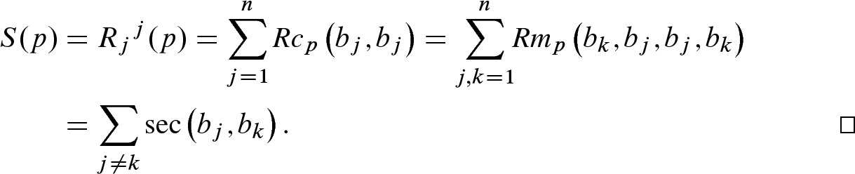
../images/56724_2_En_8_Chapter/56724_2_En_8_Equ123_HTML.png

One consequence of this proposition is that if (M, g) is a Riemannian manifold in which all sectional curvatures are positive, then the Ricci and scalar curvatures are both positive as well. The analogous statement holds if “positive" is replaced by “negative," “nonpositive," or “nonnegative."

If the opposite sign convention is chosen for the curvature tensor, then the right-hand side of formula (8.28) has to be adjusted accordingly, with $$ Rm _p (v,w,v, w)$$ taking the place of $$ Rm _p (v,w,w, v)$$ . This is so that whatever sign convention is chosen for the curvature tensor, the notion of positive or negative sectional, Ricci, or scalar curvature has the same meaning for everyone.

Sectional Curvatures of the Model Spaces

We can now compute the sectional curvatures of our three families of frame-homogeneous model spaces. A Riemannian metric or Riemannian manifold is said to have constant sectional curvature if the sectional curvatures are the same for all planes at all points.

Lemma 8.33.

If a Riemannian manifold (M, g) is frame-homogeneous, then it has constant sectional curvature.

Proof.

Frame homogeneity implies, in particular, that given two 2-planes at the same or different points, there is an isometry taking one to the other. The result follows from the isometry invariance of the curvature tensor. $\square$

Thus to compute the sectional curvature of one of our model spaces, it suffices to compute the sectional curvature for one plane at one point in each space.

Theorem 8.34

(Sectional Curvatures of the Model Spaces). The following Riemannian manifolds have the indicated constant sectional curvatures:

(a)
$\big (\mathbb {R}^n,\bar{g}\big )$ has constant sectional curvature 0.
(b)
$\big (\mathbb S^n(R), \mathring{g}_R\big )$ has constant sectional curvature .
(c)
$\big (\mathbb H^n(R), \breve{g}_R\big )$ has constant sectional curvature .

Proof.

First we consider the simplest case: Euclidean space. Since the curvature tensor of $\mathbb {R}^n$ is identically zero, clearly all sectional curvatures are zero. This is also easy to see geometrically, since each plane section is actually a plane, which has zero Gaussian curvature.

Next consider the sphere $\mathbb S^n(R)$ . We need only compute the sectional curvature of the plane $\varPi$ spanned by $(\partial _1,\partial _2)$ at the point $(0,\dots , 0,1)$ . The geodesics with initial velocities in $\varPi$ are great circles in the $(x^1,x^2,x^{n+1})$ subspace. Therefore $S_\varPi$ is isometric to the round 2-sphere of radius R embedded in $\mathbb {R}^3$ . As Example 8.25 showed, $\mathbb S^2(R)$ has Gaussian curvature $$1/R^2$$ . Therefore $\mathbb S^n(R)$ has constant sectional curvature equal to .

Finally, the proof for hyperbolic spaces is left to Problem 8-28. $\square$

Note that for every real number c, exactly one of the model spaces listed above has constant sectional curvature c. These spaces will play vital roles in our comparison and local-to-global theorems in the last two chapters of the book.

$\blacktriangleright$ Exercise 8.35. Show that the metric on real projective space $\mathbb {R}\mathbb P^n$ defined in Example 2.34 has constant positive sectional curvature.

Since the sectional curvatures determine the curvature tensor, one would expect to have an explicit formula for the full curvature tensor when the sectional curvature is constant. Such a formula is provided in the following proposition.

Proposition 8.36.

A Riemannian metric g has constant sectional curvature c if and only if its curvature tensor satisfies

../images/56724_2_En_8_Chapter/56724_2_En_8_Equ124_HTML.png

In this case, the Ricci tensor and scalar curvature of g are given by the formulas

$\begin{aligned} Rc = (n-1)cg;\qquad S = n(n-1)c, \end{aligned}$

and the Riemann curvature endomorphism is

$\begin{aligned} R(v,w)x = c\big ( \langle w,x\rangle v - \langle v, x\rangle w \big ). \end{aligned}$

In terms of any basis,

$\begin{aligned} R_{ijkl} = c(g_{il}g_{jk} - g_{ik}g_{jl});\qquad R_{ij} = (n-1) c g_{ij}. \end{aligned}$

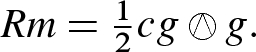
Proof.

Problem 8-29. $\square$

The basic concepts of Riemannian metrics and sectional curvatures in arbitrary dimensions were introduced by Bernhard Riemann in a famous 1854 lecture at Göttingen University [Spi97, Vol. II, Chap. 4]. These were just a few of the seminal accomplishments in his tragically short life.

Problems

8-1.
Suppose U is an open set in $\mathbb {R}^n$ and $f:U\mathrel {\rightarrow }\mathbb {R}$ is a smooth function. Let $M=\{(x, f(x)): x\in U\}\subseteq \mathbb {R}^{n+1}$ be the graph of f, endowed with the induced Riemannian metric and upward unit normal (see Example 2.19).
1. (a)
  Compute the components of the shape operator in graph coordinates, in terms of f and its partial derivatives.
2. (b)
  Let $M\subseteq \mathbb {R}^{n+1}$ be the n-dimensional paraboloid defined as the graph of . Compute the principal curvatures of M.
  (Used on p. 361.)
8-2.
Let (M, g) be an embedded Riemannian hypersurface in a Riemannian manifold $\big ({{\widetilde{M}}},{\tilde{g}}\big )$ , let F be a local defining function for M, and let $N={{\,\mathrm{grad}\,}}F/|{{\,\mathrm{grad}\,}}F|$ .
1. (a)
  Show that the scalar second fundamental form of M with respect to the unit normal N is given by
  $\begin{aligned} h(X, Y) = - \frac{\tilde{\nabla }^2 F(X, Y)}{|{{\,\mathrm{grad}\,}}F|} \end{aligned}$
  for all $X, Y\in \mathfrak X(M)$ .
2. (b)
  Show that the mean curvature of M is given by
  $\begin{aligned} H = - \frac{1}{n}{{\,\mathrm{div}\,}}_{\tilde{g}}\bigg (\frac{{{\,\mathrm{grad}\,}}F}{|{{\,\mathrm{grad}\,}}F|}\bigg ), \end{aligned}$
  where $n=\dim M$ and ${{\,\mathrm{div}\,}}_{\tilde{g}}$ is the divergence operator of $\tilde{g}$ (see Problem 5-14). [Hint: First prove the following linear-algebra lemma: If V is a finite-dimensional inner product space, $w\in V$ is a unit vector, and $A:V\mathrel {\rightarrow }V$ is a linear map that takes $w^\perp$ to $w^\perp$ , then $\mathrm{tr}\bigl (A|_{w^\perp }\bigr ) = \mathrm{tr}B$ , where $B:V\mathrel {\rightarrow }V$ is defined by $Bx = Ax - \langle x, w\rangle Aw$ .]
8-3.
Let C be an embedded smooth curve in the half-plane $H = \{(r, z): r>0\}$ , and let $S_C\subseteq \mathbb {R}^3$ be the surface of revolution determined by C as in Example 2.20. Let $\gamma (t)=(a(t), b(t))$ be a unit-speed local parametrization of C, and let X be the local parametrization of given by (2.11).
1. (a)
  Compute the shape operator and principal curvatures of in terms of a and b, and show that the principal directions at each point are tangent to the meridians and latitude circles.
2. (b)
  Show that the Gaussian curvature of at a point $X(t,\theta )$ is equal to .
8-4.
Show that there is a surface of revolution in $\mathbb {R}^3$ that has constant Gaussian curvature equal to 1 but does not have constant principal curvatures. [Remark: We will see in Chapter 10 that this surface is locally isometric to $\mathbb S^2$ (see Cor. 10.15), so this gives an example of two nonflat hypersurfaces in $\mathbb {R}^3$ that are locally isometric but have different principal curvatures.]
8-5.
Let $S\subseteq \mathbb {R}^3$ be the paraboloid given by , with the induced metric. Prove that S is isotropic at only one point. (Used on p. 56.)
8-6.
Suppose (M, g) is a Riemannian manifold, and $\gamma :I\mathrel {\rightarrow }M$ is a regular (but not necessarily unit-speed) curve in M. Show that the geodesic curvature of $\gamma$ at $t\in I$ is
$\begin{aligned} \kappa (t) = \frac{|\gamma '(t)\wedge D_t \gamma '(t)|}{|\gamma '(t)|^3}, \end{aligned}$
where the norm in the numerator is the one defined by (8.27). Show also that in $\mathbb {R}^3$ with the Euclidean metric, the formula can be written
$\begin{aligned} \kappa (t) = \frac{|\gamma '(t)\times \gamma ''(t)|}{|\gamma '(t)|^3}. \end{aligned}$
8-7.
For , let $M_w\subseteq \mathbb {R}^3$ be the surface of revolution obtained by revolving the curve $\gamma (t) = (w \cosh (t/w), t)$ around the z-axis, called a catenoid. Show that is a minimal surface for each w.
8-8.
For , let $C_h\subseteq \mathbb {R}^3$ be the one-dimensional submanifold $\{(x,y, z): x^2 + y^2 =1,\ z=\pm h\}$ ; it is the union of two unit circles lying in the $z=\pm h$ planes. Let $h_0=1/\sinh c$ , where c is the unique positive solution to the equation $c\tanh c = 1$ . Prove that if , then there are two distinct positive values such that the portions of the catenoids $M_{w_1}$ and $M_{w_2}$ lying in the region $|z|\le h$ are minimal surfaces with boundary (using the notation of Problem 8-7), while if , there is exactly one such value, and if , there are none. [Remark: This phenomenon can be observed experimentally. If you dip two parallel wire circles into soapy water, as long as they are close together they will form an area-minimizing soap film in the shape of a portion of a catenoid (the one with the larger “waist,” $M_{w_2}$ in the notation above). As you pull the circles apart, the “waist" of the catenoid gets smaller, until the ratio of the distance between the circles to their diameter reaches $h_0\approx 0.6627$ , at which point the film will burst and the only soap film that can be formed is two disjoint flat disks.]
8-9.
Let $M\subseteq \mathbb {R}^{n+1}$ be a Riemannian hypersurface, and let N be a smooth unit normal vector field along M. At each point $p\in M$ , $N_p\in T_p\mathbb {R}^{n+1}$ can be thought of as a unit vector in $\mathbb {R}^{n+1}$ and therefore as a point in $\mathbb S^n$ . Thus each choice of unit normal vector field defines a smooth map $\nu :M\mathrel {\rightarrow }\mathbb S^n$ , called the Gauss map of ${\varvec{M}}$ . Show that $\nu ^*dV_{\mathring{g}} = (-1)^n K\, dV_g$ , where K is the Gaussian curvature of M.
8-10.
Suppose $g=g_1\oplus g_2$ is a product metric on $M_1\times M_2$ as in (2.12). (See also Problem 7-6.)
1. (a)
  Show that for each point $p_i\in M_i$ , the submanifolds $M_1\times \{p_2\}$ and $\{p_1\}\times M_2$ are totally geodesic.
2. (b)
  Show that $\sec (\varPi )=0$ for every 2-plane $\varPi \subseteq T_{(p_1,p_2)}(M_1\times M_2)$ spanned by $v_1\in T_{p_1}M_1$ and $v_2\in T_{p_2}M_2$ .
3. (c)
  Show that if and both have nonnegative sectional curvature, then $M_1\times M_2$ does too; and if and both have nonpositive sectional curvature, then $M_1\times M_2$ does too.
4. (d)
  Now suppose has constant sectional curvature for ; let $n_i = \dim M_i$ . Show that (M, g) is Einstein if and only if ${c_1(n_1-1)} = {c_2(n_2-1)}$ ; and (M, g) has constant sectional curvature if and only if or .
  (Used on p. 366.)
8-11.
Suppose $M\subseteq \mathbb {R}^3$ is a smooth surface, $p\in M$ , and is a normal vector to M at p. Show that if $\varPi \subseteq \mathbb {R}^3$ is any affine plane containing p and parallel to , then there is a neighborhood U of p in $\mathbb {R}^3$ such that $M\cap \varPi \cap U$ is a smooth embedded curve in $\varPi$ , and the principal curvatures of M at p are equal to the minimum and maximum signed Euclidean curvatures of these curves as $\varPi$ varies. [Remark: This justifies the informal recipe for computing principal curvatures given in Chapter 1.]
8-12.
Suppose $\pi :\big ({{\widetilde{M}}},{\tilde{g}}\big )\mathrel {\rightarrow }(M, g)$ is a Riemannian submersion, and $\big ({{\widetilde{M}}},{\tilde{g}}\big )$ has all sectional curvatures bounded below by a constant c. Use O’Neill’s formula (Problem 7-14) to show that the sectional curvatures of (M, g) are bounded below by the same constant.
8-13.
Let $p:\mathbb S^{2n+1}\mathrel {\rightarrow }\mathbb C\mathbb P^n$ be the Riemannian submersion described in Example 2.30. In this problem, we identify $\mathbb C^{n+1}$ with $\mathbb {R}^{2n+2}$ by means of coordinates $(x^1,y^1,\dots , x^{n+1}, y^{n+1})$ defined by .
1. (a)
  Show that the vector field
  $\begin{aligned} S = x^j\frac{\partial }{\partial y^j} - y^j\frac{\partial }{\partial x^j} \end{aligned}$
  on $\mathbb C^{n+1}$ is tangent to $\mathbb S^{2n+1}$ and spans the vertical space at each point $z\in \mathbb S^{2n+1}$ . (The implicit summation here is from 1 to .)
2. (b)
  Show that for all horizontal vector fields W, Z on $\mathbb S^{2n+1}$ ,
  $\begin{aligned}{}[W,Z]^V = -d\omega (W, Z) S = 2\langle W, JZ\rangle S, \end{aligned}$
  where $\omega$ is the 1-form on $\mathbb C^{n+1}$ given by
  $\begin{aligned} \omega = S^\flat = \sum _j x^j \, dy^j - y^j\, dx^j, \end{aligned}$
  and $J:T\mathbb C^{n+1}\mathrel {\rightarrow }T\mathbb C^{n+1}$ is the real-linear orthogonal map given by
  $\begin{aligned} J\left( a^j \frac{\partial }{\partial x^j} + b^j \frac{\partial }{\partial y^j}\right) =a^j \frac{\partial }{\partial y^j}-b^j \frac{\partial }{\partial x^j}. \end{aligned}$
  (This is just multiplication by $i=\sqrt{-1}$ in complex coordinates. Notice that $J\circ J = - \mathrm{Id}$ .)
3. (c)
  Using O’Neill’s formula (Problem 7-14), show that the curvature tensor of $\mathbb C\mathbb P^n$ satisfies
  $\begin{aligned} \begin{aligned} Rm (w,x,y, z)&= \langle \tilde{w},\tilde{z}\rangle \langle \tilde{x},\tilde{y}\rangle - \langle \tilde{w},\tilde{y}\rangle \langle \tilde{x},\tilde{z}\rangle \\&\quad - 2 \langle \tilde{w}, J \tilde{x}\rangle \langle \tilde{y}, J \tilde{z}\rangle - \langle \tilde{w}, J \tilde{y}\rangle \langle \tilde{x}, J \tilde{z}\rangle \\&\quad + \langle \tilde{w}, J \tilde{z}\rangle \langle \tilde{x}, J \tilde{y}\rangle , \end{aligned} \end{aligned}$
  for every $q\in \mathbb C\mathbb P^n$ and $w,x,y, z\in T_q\mathbb C\mathbb P^n$ , where $\tilde{w},\tilde{x},\tilde{y},\tilde{z}$ are horizontal lifts of w, x, y, z to an arbitrary point $\tilde{q}\in p^{-1}(q)\subseteq \mathbb S^{2n+1}$ .
4. (d)
  Using the notation of part (c), show that for orthonormal vectors $w, x\in T_q\mathbb C\mathbb P^n$ , the sectional curvature of the plane spanned by $\{w, x\}$ is
  $\begin{aligned} \sec (w, x) = 1 + 3\bigl \langle \tilde{w}, J\tilde{x}\bigr \rangle ^2. \end{aligned}$
5. (e)
  Show that for $n\ge 2$ , the sectional curvatures at each point of $\mathbb C\mathbb P^n$ take on all values between 1 and 4, inclusive, and conclude that $\mathbb C\mathbb P^n$ is not frame-homogeneous.
6. (f)
  Compute the Gaussian curvature of $\mathbb C\mathbb P^1$ .
  (Used on pp. 56, 262, 367.)
8-14.
Show that a Riemannian 3-manifold is Einstein if and only if it has constant sectional curvature.
8-15.
Suppose (M, g) is a 3-dimensional Riemannian manifold that is homogeneous and isotropic. Show that g has constant sectional curvature. Show that the analogous result in dimension 4 is not true. [Hint: See Problem 8-13.]
8-16.
For each , let be the Berger metric on $\mathrm{SU}(2)$ defined in Problem 3-10. Compute the sectional curvatures with respect to of the planes spanned by (X, Y), (Y, Z), and (Z, X). Prove that if $a\ne 1$ , then $(\mathrm{SU}(2), g_a)$ is homogeneous but not isotropic anywhere. (Used on p. 56.)
8-17.
Let G be a Lie group with a bi-invariant metric g (see Problem 7-13).
1. (a)
  Suppose X and Y are orthonormal elements of $\mathrm{Lie}(G)$ . Show that $\sec (X_p, Y_p) = \tfrac{1}{4}\big |[X, Y]\big |^2$ for each $p\in G$ , and conclude that the sectional curvatures of (G, g) are all nonnegative.
2. (b)
  Show that every Lie subgroup of G is totally geodesic in G.
3. (c)
  Now suppose G is connected. Show that G is flat if and only if it is abelian.
  (Used on p. 282.)
8-18.
Suppose (M, g) is a Riemannian hypersurface in a Riemannian manifold $\bigl ({{\widetilde{M}}},\tilde{g}\bigr )$ , and N is a unit normal vector field along M. We say that M is convex (with respect to N) if its scalar second fundamental form satisfies $h(v, v)\le 0$ for all $v\in TM$ . Show that if M is convex and ${{\widetilde{M}}}$ has sectional curvatures bounded below by a constant c, then all sectional curvatures of M are bounded below by c.
8-19.
Suppose (M, g) is a Riemannian hypersurface in an -dimensional Lorentz manifold $\big ({{\widetilde{M}}},{\tilde{g}}\big )$ , and N is a smooth unit normal vector field along M. Define the scalar second fundamental form h and the shape operator s by requiring that $\mathrm {II}(X,Y) = h(X, Y)N$ and $\langle sX,Y\rangle = h(X, Y)$ for all $X, Y\in \mathfrak X(M)$ . Prove the following Lorentz analogues of the formulas of Theorem 8.13 (with notation as in that theorem):
1. (a)
  Gauss Formula: $\tilde{\nabla }_XY = \nabla _XY + h(X, Y)N$ .
2. (b)
  Gauss Formula for a Curve: $\tilde{D}_tX = {D_tX} + h(\gamma ', X)N$ .
3. (c)
  Weingarten Equation: $\tilde{\nabla }_XN = sX$ .
4. (d)
  Gauss Equation: .
5. (e)
  Codazzi Equation: .
8-20.
Suppose $\big ({{\widetilde{M}}},{\tilde{g}}\big )$ is an -dimensional Lorentz manifold, and assume that ${\tilde{g}}$ satisfies the Einstein field equation with a cosmological constant: $\smash {\widetilde{ Rc } - \frac{1}{2} \tilde{S} \tilde{g} + \Lambda \tilde{g}} = T$ , where $\Lambda$ is a constant and T is a smooth symmetric 2-tensor field (see p. 211). Let (M, g) be a Riemannian hypersurface in ${{\widetilde{M}}}$ , and let h be its scalar second fundamental form as defined in Problem 8-19. Use the results of Problem 8-19 to show that g and h satisfy the following Einstein constraint equations on M:
$\begin{aligned} S - 2\Lambda - |h|_g^2 + \left( {{\,\mathrm{tr}\,}}_g h\right) ^2&= 2 \rho ,\\ {{\,\mathrm{div}\,}}h - d\left( {{\,\mathrm{tr}\,}}_g h\right)&= J, \end{aligned}$
where S is the scalar curvature of g, ${{\,\mathrm{div}\,}}h$ the divergence of h with respect to g as defined in Problem 5-16, $\rho$ is the function $\rho =T(N, N)$ , and J is the 1-form . [Remark: When J and $\rho$ are both zero, these equations, known as the vacuum Einstein constraint equations, are necessary conditions for g and h to be the metric and second fundamental form of a Riemannian hypersurface in an -dimensional Lorentz manifold satisfying the vacuum Einstein field equation with cosmological constant $\Lambda$ . It was proved in 1950 by Yvonne Choquet-Bruhat that these conditions are also sufficient; for a proof, see [CB09, pp. 166–168].]
8-21.
For every linear endomorphism $A:\mathbb {R}^n\mathrel {\rightarrow }\mathbb {R}^n$ , the associated quadratic form is the function $Q:\mathbb {R}^n\mathrel {\rightarrow }\mathbb {R}$ defined by $Q(x) = \langle A x,\, x \rangle$ . Prove that
$\begin{aligned} \int _{\mathbb S^{n-1}} Q \, dV_{\mathring{g}} = \frac{1}{n}({{\,\mathrm{tr}\,}}A)\mathrm{Vol}\big (\mathbb S^{n-1}\big ). \end{aligned}$
[Hint: Show that $\int _{\mathbb S^{n-1}} x^i x^j\, dV_{\mathring{g}}=0$ when $i\ne j$ by examining the effect of the isometry
$\begin{aligned} (x^1,\dots , x^i, \dots , x^j, \dots , x^n)\mapsto (x^1,\dots , x^j, \dots , -x^i, \dots , x^n), \end{aligned}$
and compute $\int _{\mathbb S^{n-1}}\big (x^i\big )^2\, dV_{\mathring{g}}$ using the fact that $\sum _i \big (x^i\big )^2=1$ on the sphere.] [Remark: It is a standard fact of linear algebra that the trace of A is independent of the choice of basis. This gives a geometric interpretation to the trace as n times the average value of the associated quadratic form Q.]
(Used on p. 313.)
8-22.
Let (M, g) be a Riemannian n-manifold and $p\in M$ . Proposition 8.32 gave a geometric interpretation of the Ricci curvature at p based on a choice of orthonormal basis. This problem describes an interpretation that does not refer to a basis. For each unit vector $v\in T_pM$ , prove that
$\begin{aligned} Rc_p(v, v) = \frac{n-1}{\mathrm{Vol}\big (\mathbb S^{n-2}\big )}\int _{w\in S_v^\perp } \sec (v, w)\, dV_{\hat{g}}, \end{aligned}$
where $S_v^\perp$ denotes the set of unit vectors in that are orthogonal to v and $\hat{g}$ denotes the Riemannian metric on $S_v^\perp$ induced from the flat metric on . [Hint: Use Problem 8-21.]
8-23.
Suppose (M, g) is a connected n-dimensional Riemannian manifold, and a Lie group G acts isometrically and effectively on M. Problem 5-12 showed that $\dim G \le n(n+1)/2$ . Prove that if equality holds, then g has constant sectional curvature.
8-24.
Let (M, g) be a connected Riemannian manifold. Recall the definition of k-point homogeneous from Problem 6-18. Prove the following:
1. (a)
  If (M, g) is homogeneous, then it has constant scalar curvature.
2. (b)
  If (M, g) is 2-point homogeneous, then it is Einstein.
3. (c)
  If (M, g) is 3-point homogeneous, then it has constant sectional curvature.
8-25.
For , suppose is a Riemannian manifold of dimension $n_i\ge 2$ with constant sectional curvature ; and let $g = g_1\oplus g_2$ be the product metric on $M = M_1\times M_2$ . Show that the Weyl tensor of g is given by
where and $h_i = \pi _i^*g_i$ for . Conclude that (M, g) is locally conformally flat if and only if . (See also Problem 7-6.)
(Used on p. 67.)
8-26.
Let (M, g) be a 4-dimensional Riemannian manifold. Given $p\in M$ and an orthonormal basis for , prove that the Weyl tensor at p satisfies
$\begin{aligned} W_{1221} = \frac{1}{3} (k_{12} + k_{34}) - \frac{1}{6} (k_{13} + k_{14} + k_{23} + k_{24}), \end{aligned}$
where $k_{ij}$ is the sectional curvature of the plane spanned by $\left( b_i, b_j\right)$ .
8-27.
Prove that the Fubini–Study metric on $\mathbb C\mathbb P^2$ is not locally conformally flat. [Hint: Use Problems 8-13 and 8-26.]
8-28.
Complete the proof of Theorem 8.34 by showing in two ways that the hyperbolic space of radius R has constant sectional curvature equal to .
1. (a)
  In the hyperboloid model, compute the second fundamental form of $\mathbb H^n(R)\subseteq \mathbb {R}^{n, 1}$ at the point $(0,\dots , 0,R)$ , and use either the general form of the Gauss equation (Thm. 8.5) or the formulas of Problem 8-19.
2. (b)
  In the Poincaré ball model, use formula (7.44) for the conformal transformation of the curvature to compute the Riemann curvature tensor at the origin.
8-29.
Prove Proposition 8.36 (curvature tensors on constant-curvature spaces).
8-30.
Suppose $M\subseteq \mathbb {R}^{n+1}$ is a hypersurface with the induced Riemannian metric. Show that the Ricci tensor of M satisfies
$\begin{aligned} Rc (v, w) = \big \langle n H sv - s^2v,\ w\big \rangle , \end{aligned}$
where H and s are the mean curvature and shape operator of M, respectively, and .
8-31.
For $1< k\le n$ , show that any k points in the hyperbolic space $\mathbb H^n(R)$ lie in a totally geodesic -dimensional submanifold, which is isometric to $\mathbb H^{k-1}(R)$ .
8-32.
Suppose (M, g) is a Riemannian manifold and G is a Lie group acting smoothly and isometrically on M. Let $S\subseteq M$ be the fixed point set of G, that is, the set of points $p\in M$ such that $\varphi (p)=p$ for all $\varphi \in G$ . Show that each connected component of S is a smoothly embedded totally geodesic submanifold of M. (The reason for restricting to a single connected component is that different components may have different dimensions.)
8-33.
Suppose (M, g) is a Riemannian manifold. Let $\Lambda ^2(TM)$ denote the bundle of 2-vectors (alternating contravariant 2-tensors) on M.
1. (a)
  Show that there is a unique fiber metric on $\Lambda ^2(TM)$ whose associated norm satisfies
  $\begin{aligned} |w\wedge x|^2 = |w|^2 |x|^2 - \langle w, x\rangle ^2 \end{aligned}$
  for all tangent vectors w, x at every point $q\in M$ .
2. (b)
  Show that there is a unique bundle endomorphism $\mathscr {R}:\Lambda ^2(TM) \mathrel {\rightarrow } \Lambda ^2(TM)$ , called the curvature operator of g, that satisfies
  $\begin{aligned} \big \langle \mathscr {R}(w\wedge x), y\wedge z\big \rangle = - Rm (w,x,y, z) \end{aligned}$
  
  (8.30)
  for all tangent vectors w, x, y, z at a point of M, where the inner product on the left-hand side is the one described in part (a).
3. (c)
  A Riemannian metric is said to have positive curvature operator if $\mathscr {R}$ is positive definite, and negative curvature operator if $\mathscr {R}$ is negative definite. Show that positive curvature operator implies positive sectional curvature, and negative curvature operator implies negative sectional curvature. [Remark: This is the reason for the negative sign in (8.30). If the Riemann curvature tensor is defined as the negative of ours, the negative sign should be omitted.]
4. (d)
  Show that the converse need not be true, by using the results of Problem 8-13 to compute the following expression on $\mathbb C\mathbb P^2$ with the Fubini–Study metric:
  $\begin{aligned} \big \langle \mathscr {R}(w\wedge x+ y\wedge z),\ w\wedge x + y\wedge z\big \rangle , \end{aligned}$
  where w, x, y, z are orthonormal vectors at an arbitrary point of $\mathbb C\mathbb P^2$ , chosen so that their horizontal lifts satisfy $\tilde{y} = J\tilde{w}$ and $\tilde{z}=J\tilde{x}$ .