In this chapter we officially define Riemannian metrics, and discuss some of the basic computational techniques associated with them. After the definitions, we describe a few standard methods for constructing Riemannian manifolds as submanifolds, products, and quotients of other Riemannian manifolds. Then we introduce some of the elementary geometric constructions provided by Riemannian metrics, the most important of which is the Riemannian distance function, which turns every connected Riemannian manifold into a metric space.
At the end of the chapter, we discuss some important generalizations of Riemannian metrics—most importantly, the pseudo-Riemannian metrics, followed by brief mentions of sub-Riemannian and Finsler metrics.
Before you read this chapter, it would be a good idea to skim through the three appendices after Chapter 12 to get an idea of the prerequisite material that will be assumed throughout this book.
Definitions
 can be derived from its dot product, which is defined for
  and
and  by
by
 is a map
  , typically written
  , that satisfies the following properties for all
  and
and  :
:- (i)
Symmetry:
 .
. - (ii)
Bilinearity:
 .
. - (iii)
Positive Definiteness:
 , with equality if and only if
  .
.
A vector space endowed with a specific inner product is called an inner product space.
 as
as
Lemma 2.1
 is an inner product on a vector space V. Then for all
  ,
,
 Exercise 2.2. Prove the preceding lemma.
 is defined as the unique
 ![$$\theta \in [0,\pi ]$$](../images/56724_2_En_2_Chapter/56724_2_En_2_Chapter_TeX_IEq19.png) satisfying
satisfying
 are said to be orthogonal if
  , which means that either their angle is
  or one of the vectors is zero. If
  is a linear subspace, the set
  , consisting of all vectors in V that are orthogonal to every vector in S, is also a linear subspace, called the orthogonal complement of
  .
.Vectors  are called orthonormal if they are of length 1 and pairwise orthogonal, or equivalently if
  (where
  is the Kronecker delta symbol defined in Appendix B; see (B.1)). The following well-known proposition shows that every finite-dimensional inner product space has an orthonormal basis.
Proposition 2.3
 is any ordered basis for V. Then there is an orthonormal ordered basis
  satisfying the following conditions:
Proof.
 are defined recursively by

 and
and  for each
  , the denominators are all nonzero. These vectors satisfy (2.4) by construction, and are orthonormal by direct computation.
If two vector spaces V and W are both equipped with inner products, denoted by  and
and  , respectively, then a map
  is called a linear isometry if it is a vector space isomorphism that preserves inner products:
  . If V and W are inner product spaces of dimension n, then given any choices of orthonormal bases
  for V and
  for W, the linear map
  determined by
  is easily seen to be a linear isometry. Thus all inner product spaces of the same finite dimension are linearly isometric to each other.
Riemannian Metrics
To extend these geometric ideas to abstract smooth manifolds, we define a structure that amounts to a smoothly varying choice of inner product on each tangent space.
Let M be a smooth manifold. A Riemannian metric on M is a smooth covariant 2-tensor field  whose value
  at each
  is an inner product on
  ; thus g is a symmetric 2-tensor field that is positive definite in the sense that
  for each
  and each
  , with equality if and only if
  . A Riemannian manifold is a pair (M, g), where M is a smooth manifold and g is a specific choice of Riemannian metric on M. If M is understood to be endowed with a specific Riemannian metric, we sometimes say “M is a Riemannian manifold.”
The next proposition shows that Riemannian metrics exist in great abundance.
Proposition 2.4.
Every smooth manifold admits a Riemannian metric.
 Exercise 2.5. Use a partition of unity to prove the preceding proposition.
We will give a number of examples of Riemannian metrics, along with several systematic methods for constructing them, later in this chapter and in the next.
If M is a smooth manifold with boundary, a Riemannian metric on M is defined in exactly the same way: a smooth symmetric 2-tensor field g that is positive definite everywhere. A Riemannian manifold with boundary is a pair (M, g), where M is a smooth manifold with boundary and g is a Riemannian metric on M. Many of the results we will discuss in this book work equally well for manifolds with or without boundary, with the same proofs, and in such cases we will state them in that generality. But when the treatment of a boundary would involve additional difficulties, we will generally restrict attention to the case of manifolds without boundary, since that is our primary interest. Many problems involving Riemannian manifolds with boundary can be addressed by embedding into a larger manifold without boundary and extending the Riemannian metric arbitrarily to the larger manifold; see Proposition A.31 in Appendix A.
A Riemannian metric is not the same as a metric in the sense of metric spaces (though, as we will see later in this chapter, the two concepts are related). In this book, when we use the word “metric” without further qualification, it always refers to a Riemannian metric.
 is an inner product on
  for each
  , we often use the following angle-bracket notation for
  :
:

 is denoted by
  . If the metric is understood, we sometimes omit it from the notation, and write
  and |v| in place of
  and
and  , respectively.
The starting point for Riemannian geometry is the following fundamental example.
Example 2.6
 on
on  whose value at each
  is just the usual dot product on
  under the natural identification
  . This means that for
  written in standard coordinates
  as
as  ,
,  , we have
 as a Riemannian manifold, we always assume we are using the Euclidean metric unless otherwise specified. //
Isometries
Suppose (M, g) and  are Riemannian manifolds with or without boundary. An isometry from
  to
to  is a diffeomorphism
  such that
  . Unwinding the definitions shows that this is equivalent to the requirement that
  be a smooth bijection and each differential
  be a linear isometry. We say (M, g) and
  are isometric if there exists an isometry between them.
A composition of isometries and the inverse of an isometry are again isometries, so being isometric is an equivalence relation on the class of Riemannian manifolds with or without boundary. Our subject, Riemannian geometry, is concerned primarily with properties of Riemannian manifolds that are preserved by isometries.
If (M, g) and  are Riemannian manifolds, a map
  is a local isometry if each point
  has a neighborhood U such that
  is an isometry onto an open subset of
  .
.
 Exercise 2.7. Prove that if (M, g) and
  are Riemannian manifolds of the same dimension, a smooth map
  is a local isometry if and only if
  .
.
A Riemannian n-manifold is said to be flat if it is locally isometric to a Euclidean space, that is, if every point has a neighborhood that is isometric to an open set in  with its Euclidean metric. Problem 2-1 shows that all Riemannian 1-manifolds are flat; but we will see later that this is far from the case in higher dimensions.
An isometry from (M, g) to itself is called an isometry of  . The set of all isometries of (M, g) is a group under composition, called the isometry group of
  ; it is denoted by
  , or sometimes just
  if the metric is understood.
A deep theorem of Sumner B. Myers and Norman E. Steenrod [MS39] shows that if M has finitely many components, then  has a topology and smooth structure making it into a finite-dimensional Lie group acting smoothly on M. We will neither prove nor use the Myers–Steenrod theorem, but if you are interested, a good source for the proof is [Kob72].
Local Representations for Metrics
 are any smooth local coordinates on an open subset
  , then g can be written locally in U as
 smooth functions
  for
for  . (Here and throughout the book, we use the Einstein summation convention; see p. 375.) The component functions of this tensor field constitute a matrix-valued function
  , characterized by
  , where
  is the ith coordinate vector field; this matrix is symmetric in i and j and depends smoothly on
  . If
. If  is a vector in
  such that
  , it follows that
  , which implies
  ; thus the matrix
  is always nonsingular. The notation for g can be shortened by expressing it in terms of the symmetric product (see Appendix B): using the symmetry of
  , we compute
 (Example 2.6) can be expressed in standard coordinates in several ways:
 in these coordinates is thus
  .
. is any smooth local frame for TM on an open subset
  and
and  is its dual coframe, we can write g locally in U as
 , and the matrix-valued function
  is symmetric and smooth as before.
A Riemannian metric g acts on smooth vector fields  to yield a real-valued function
  . In terms of any smooth local frame, this function is expressed locally by
  and therefore is smooth. Similarly, we obtain a nonnegative real-valued function
  , which is continuous everywhere and smooth on the open subset where
  .
.
 for M on an open set U is said to be an orthonormal frame if the vectors
  are an orthonormal basis for
  at each
  . Equivalently,
  is an orthonormal frame if and only if

 denotes the symmetric product
  .
.Proposition 2.8
(Existence of Orthonormal Frames). Let (M, g) be a Riemannian n-manifold with or without boundary. If  is any smooth local frame for TM over an open subset
  , then there is a smooth orthonormal frame
  over U such that
  for each
  and each
  . In particular, for every
  , there is a smooth orthonormal frame
  defined on some neighborhood of p.
Proof.
Applying the Gram–Schmidt algorithm to the vectors  at each
  , we obtain an ordered n-tuple of rough orthonormal vector fields
  over U satisfying the span conditions. Because the vectors whose norms appear in the denominators of (2.5)–(2.6) are nowhere vanishing, those formulas show that each vector field
  is smooth. The last statement of the proposition follows by applying this construction to any smooth local frame in a neighborhood of p.
Warning: A common mistake made by beginners is to assume that one can find coordinates near p such that the coordinate frame  is orthonormal. Proposition 2.8 does not show this. In fact, as we will see in Chapter 7, this is possible only when the metric is flat, that is, locally isometric to the Euclidean metric.
 consisting of unit vectors:
Proposition 2.9
(Properties of the Unit Tangent Bundle). If (M, g) is a Riemannian manifold with or without boundary, its unit tangent bundle UTM is a smooth, properly embedded codimension-1 submanifold with boundary in TM, with  (where
  is the canonical projection). The unit tangent bundle is connected if and only if M is connected, and compact if and only if M is compact.
 Exercise 2.10. Use local orthonormal frames to prove the preceding proposition.
Methods for Constructing Riemannian Metrics
Many examples of Riemannian manifolds arise naturally as submanifolds, products, and quotients of other Riemannian manifolds. In this section, we introduce some of the tools for constructing such metrics.
Riemannian Submanifolds
Every submanifold of a Riemannian manifold automatically inherits a Riemannian metric, and many interesting Riemannian metrics are defined in this way. The key fact is the following lemma.
Lemma 2.11.
Suppose  is a Riemannian manifold with or without boundary, M is a smooth manifold with or without boundary, and
  is a smooth map. The smooth 2-tensor field
  is a Riemannian metric on M if and only if F is an immersion.
 Exercise 2.12. Prove Lemma 2.11.
Suppose  is a Riemannian manifold with or without boundary. Given a smooth immersion
  , the metric
  is called the metric induced by
  . On the other hand, if M is already endowed with a given Riemannian metric g, an immersion or embedding
  satisfying
  is called an isometric immersion or isometric embedding, respectively. Which terminology is used depends on whether the metric on M is considered to be given independently of the immersion or not.
The most important examples of induced metrics occur on submanifolds. Suppose  is an (immersed or embedded) submanifold, with or without boundary. The induced metric on
  is the metric
  induced by the inclusion map
  . With this metric, M is called a Riemannian submanifold (or Riemannian submanifold with boundary) of
  . We always consider submanifolds (with or without boundary) of Riemannian manifolds to be endowed with the induced metrics unless otherwise specified.
 , then for every
  and
and  , the definition of the induced metric reads
 with its image in
  under
under  , and think of
  as an inclusion map, what this really amounts to is
  for
for  . In other words, the induced metric g is just the restriction of
  to vectors tangent to M. Many of the examples of Riemannian metrics that we will encounter are obtained in this way, starting with the following.
Example 2.13
(Spheres). For each positive integer n, the unit n-sphere  is an embedded n-dimensional submanifold. The Riemannian metric induced on
  by the Euclidean metric is denoted by
  and known as the round metric or standard metric on
  . //
. //
The next lemma describes one of the most important tools for studying Riemannian submanifolds. If  is an m-dimensional smooth Riemannian manifold and
  is an n-dimensional submanifold (both with or without boundary), a local frame
  for
for  on an open subset
 ![$${\smash [t]{\tilde{U}}}\subseteq {{\widetilde{M}}}$$](../images/56724_2_En_2_Chapter/56724_2_En_2_Chapter_TeX_IEq195.png) is said to be adapted to
is said to be adapted to  if the first n vector fields
  are tangent to M. In case
  has empty boundary (so that slice coordinates are available), adapted local orthonormal frames are easy to find.
Proposition 2.14
(Existence of Adapted Orthonormal Frames). Let  be a Riemannian manifold (without boundary), and let
  be an embedded smooth submanifold with or without boundary. Given
  , there exist a neighborhood
 ![$${\smash [t]{\tilde{U}}}$$](../images/56724_2_En_2_Chapter/56724_2_En_2_Chapter_TeX_IEq202.png) of p in
of p in  and a smooth orthonormal frame for
  on
on ![$${\smash [t]{\tilde{U}}}$$](../images/56724_2_En_2_Chapter/56724_2_En_2_Chapter_TeX_IEq205.png) that is adapted to M.
that is adapted to M.
 Exercise 2.15. Prove the preceding proposition. [Hint: Apply the Gram–Schmidt algorithm to a coordinate frame in slice coordinates (see Prop. A.22).]
 is a Riemannian manifold and
  is a smooth submanifold with or without boundary in
  . Given
  , a vector
  is said to be normal to
  if
if  for every
  . The space of all vectors normal to M at p is a subspace of
  , called the normal space at
  and denoted by
  . At each
  , the ambient tangent space
  splits as an orthogonal direct sum
  . A section N of the ambient tangent bundle
  is called a normal vector field along
  if
if  for each
  . The set

 .
.Proposition 2.16
 is a Riemannian m-manifold and
  is an immersed or embedded n-dimensional submanifold with or without boundary, then
  is a smooth rank-
 vector subbundle of the ambient tangent bundle
  . There are smooth bundle homomorphisms
 restrict to orthogonal projections from
  to
to  and
and  , respectively.
Proof.
Given any point  , Theorem A.16 shows that there is a neighborhood U of p in M that is embedded in
  , and then Proposition 2.14 shows that there is a smooth orthonormal frame
  that is adapted to U on some neighborhood
 ![$${\smash [t]{\tilde{U}}}$$](../images/56724_2_En_2_Chapter/56724_2_En_2_Chapter_TeX_IEq239.png) of p in
of p in  . This means that the restrictions of
  to
to ![$${\smash [t]{\tilde{U}}}\cap U$$](../images/56724_2_En_2_Chapter/56724_2_En_2_Chapter_TeX_IEq242.png) form a local orthonormal frame for M. Given such an adapted frame, the restrictions of the last
form a local orthonormal frame for M. Given such an adapted frame, the restrictions of the last  vector fields
  to M form a smooth local frame for
  , so it follows from Lemma A.34 that
  is a smooth subbundle.
 and
and  are defined pointwise as orthogonal projections onto the tangent and normal spaces, respectively, which shows that they are uniquely defined. In terms of an adapted orthonormal frame, they can be written

In case  is a manifold with boundary, the preceding constructions do not always work, because there is not a fully general construction of slice coordinates in that case. However, there is a satisfactory result in case the submanifold is the boundary itself, using boundary coordinates in place of slice coordinates.
Suppose (M, g) is a Riemannian manifold with boundary. We will always consider  to be a Riemannian submanifold with the induced metric.
Proposition 2.17
(Existence of Outward-Pointing Normal). If (M, g) is a smooth Riemannian manifold with boundary, the normal bundle to  is a smooth rank-1 vector bundle over
  , and there is a unique smooth outward-pointing unit normal vector field along all of
  .
.
 Exercise 2.18. Prove this proposition. [Hint: Use the paragraph preceding Prop. B.17 as a starting point.]
Computations on a submanifold  are usually carried out most conveniently in terms of a smooth local parametrization: this is a smooth map
  , where U is an open subset of
  (or
(or  in case M has a boundary), such that X(U) is an open subset of M, and such that X, regarded as a map from U into M, is a diffeomorphism onto its image. Note that we can think of X either as a map into M or as a map into
  ; both maps are typically denoted by the same symbol X. If we put
  and
and  , then
  is a smooth coordinate chart on M.
 and
and  is a smooth local parametrization of M. The coordinate representation of g in these coordinates is given by the following 2-tensor field on U:
 is just the map X itself, regarded as a map into
  , this is really just
  . The simplicity of the formula for the pullback of a tensor field makes this expression exceedingly easy to compute, once a coordinate expression for
  is known. For example, if M is an immersed n-dimensional Riemannian submanifold of
  and
and  is a smooth local parametrization of M, the induced metric on U is just
Example 2.19
 is an open set and
  is a smooth function, then the graph of
  is the subset
  , which is an embedded submanifold of dimension n. It has a global parametrization
  called a graph parametrization, given by
  ; the corresponding coordinates
  on M are called graph coordinates. In graph coordinates, the induced metric of
  is
is
 with the parametrization
  given by
 can be written locally as
Example 2.20
 , and suppose
  is an embedded 1-dimensional submanifold. The surface of revolution determined by C is the subset
  given by
 for C yields a smooth local parametrization for
  of the form
 is restricted to a sufficiently small open set in the plane. The t-coordinate curves
  are called meridians, and the
  -coordinate curves
  are called latitude circles. The induced metric on
  is
is
 is a unit-speed curve (meaning that
  ), this reduces to
  .
.Here are some examples of surfaces of revolution and their induced metrics.
If C is the semicircle
 , parametrized by
  for
for  , then
  is the unit sphere (minus the north and south poles). The map
  constructed above is called the spherical coordinate parametrization, and the induced metric is
  . (This example is the source of the terminology for meridians and latitude circles.)
If C is the circle
 , parametrized by
  , we obtain a torus of revolution, whose induced metric is
  .
.If C is a vertical line parametrized by
 , then
  is the unit cylinder
  , and the induced metric is
  . Note that this means that the parametrization
  is an isometric immersion. //
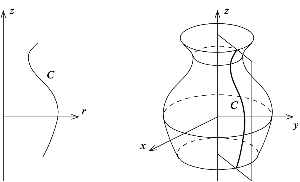
A surface of revolution
Example 2.21
(The  -Torus as a Riemannian Submanifold). The smooth covering map
  described in Example A.52 restricts to a smooth local parametrization on any sufficiently small open subset of
  , and the induced metric is equal to the Euclidean metric in
  coordinates, and therefore the induced metric on
  is flat. //
 Exercise 2.22. Verify the claims in Examples 2.19–2.21.
Riemannian Products
 and
and  are Riemannian manifolds, the product manifold
  has a natural Riemannian metric
  , called the product metric, defined by
 and
and  are elements of
  , which is naturally identified with
  . Smooth local coordinates
  for
for  and
and  for
for  give coordinates
  for
for  . In terms of these coordinates, the product metric has the local expression
  , where
  is the block diagonal matrix
 to
to  . Product metrics on products of three or more Riemannian manifolds are defined similarly.
 Exercise 2.23. Show that the induced metric on
  described in Exercise 2.21 is equal to the product metric obtained from the usual induced metric on
  .
.
 and
and  are two Riemannian manifolds, and
  is a strictly positive smooth function. The warped product
  is the product manifold
  endowed with the Riemannian metric
  , defined by
 as before. (Despite the similarity with the notation for product metrics,
  is generally not a product metric unless f is constant.) A wide variety of metrics can be constructed in this way; here are just a few examples.
Example 2.24
- (a)
With
 , the warped product
  is just the space
  with the product metric.
 - (b)
Every surface of revolution can be expressed as a warped product, as follows. Let H be the half-plane
 , let
, let  be an embedded smooth 1-dimensional submanifold, and let
  denote the corresponding surface of revolution as in Example 2.20. Endow C with the Riemannian metric induced from the Euclidean metric on H, and let
  be endowed with its standard metric. Let
  be the distance to the z-axis:
  . Then Problem 2-3 shows that
  is isometric to the warped product
  .
. - (c)
If we let
 denote the standard coordinate function on
  , then the map
  gives an isometry from the warped product
  to
to  with its Euclidean metric (see Problem 2-4). //
Riemannian Submersions
Unlike submanifolds and products of Riemannian manifolds, which automatically inherit Riemannian metrics of their own, quotients of Riemannian manifolds inherit Riemannian metrics only under very special circumstances. In this section, we see what those circumstances are.
 and M are smooth manifolds,
  is a smooth submersion, and
  is a Riemannian metric on
  . By the submersion level set theorem (Corollary A.25), each fiber
  is a properly embedded smooth submanifold of
  . At each point
  , we define two subspaces of the tangent space
  as follows: the vertical tangent space at
  is
is
 is its orthogonal complement:
 decomposes as an orthogonal direct sum
  . Note that the vertical space is well defined for every submersion, because it does not refer to the metric; but the horizontal space depends on the metric.
A vector field on  is said to be a horizontal vector field if its value at each point lies in the horizontal space at that point; a vertical vector field is defined similarly. Given a vector field X on M, a vector field
  on
on  is called a horizontal lift of
  if
if  is horizontal and
  -related to X. (The latter property means that
  for each
  .)
.)
The next proposition is the principal tool for doing computations on Riemannian submersions.
Proposition 2.25
(Properties of Horizontal Vector Fields). Let  and M be smooth manifolds, let
  be a smooth submersion, and let
  be a Riemannian metric on
  .
.
- (a)
Every smooth vector field W on
 can be expressed uniquely in the form
  , where
  is horizontal,
  is vertical, and both
  and
and  are smooth.
 - (b)
Every smooth vector field on M has a unique smooth horizontal lift to
 .
. - (c)
For every
 and
and  , there is a vector field
  whose horizontal lift
  satisfies
  .
.
Proof.
 be arbitrary. Because
  is a smooth submersion, the rank theorem (Theorem A.15) shows that there exist smooth coordinate charts
 ![$$\big ({\smash [t]{\tilde{U}}},\big (x^i\big )\big )$$](../images/56724_2_En_2_Chapter/56724_2_En_2_Chapter_TeX_IEq402.png) centered at p and
centered at p and  centered at
  in which
  has the coordinate representation
 and
and  . It follows that at each point
 ![$$q\in {\smash [t]{\tilde{U}}}$$](../images/56724_2_En_2_Chapter/56724_2_En_2_Chapter_TeX_IEq408.png) , the vertical space
, the vertical space  is spanned by the vectors
  . (It probably will not be the case, however, that the horizontal space is spanned by the other n basis vectors.) If we apply the Gram–Schmidt algorithm to the ordered frame
  , we obtain a smooth orthonormal frame
  on
on ![$${\smash [t]{\tilde{U}}}$$](../images/56724_2_En_2_Chapter/56724_2_En_2_Chapter_TeX_IEq413.png) such that
such that  is spanned by
  at each
 ![$$q\in {\smash [t]{\tilde{U}}}$$](../images/56724_2_En_2_Chapter/56724_2_En_2_Chapter_TeX_IEq416.png) . It follows that
. It follows that  is spanned by
  .
.Now let  be arbitrary. At each point
  ,
,  can be written uniquely as a sum of a vertical vector plus a horizontal vector, thus defining a decomposition
  into rough vertical and horizontal vector fields. To see that they are smooth, just note that in a neighborhood of each point we can express W in terms of a frame
  of the type constructed above as
  with smooth coefficients
  , and then it follows that
  and
and  , both of which are smooth.
The proofs of (b) and (c) are left to Problem 2-5. 
The fact that every horizontal vector at a point of  can be extended to a horizontal lift on all of
  (part (c) of the preceding proposition) is highly useful for computations. It is important to be aware, though, that not every horizontal vector field on
  is a horizontal lift, as the next exercise shows.
 Exercise 2.26. Let
  be the projection map
  , and let W be the smooth vector field
  on
on  . Show that W is horizontal, but there is no vector field on
  whose horizontal lift is equal to W.
Now we can identify some quotients of Riemannian manifolds that inherit metrics of their own. Let us begin by describing what such a metric should look like.
Suppose  and (M, g) are Riemannian manifolds, and
  is a smooth submersion. Then
  is said to be a Riemannian submersion if for each
  , the differential
  restricts to a linear isometry from
  onto
onto  . In other words,
  whenever
  .
.
Example 2.27
- (a)
The projection
 onto the first n coordinates is a Riemannian submersion if
  and
and  are both endowed with their Euclidean metrics.
 - (b)
If M and N are Riemannian manifolds and
 is endowed with the product metric, then both projections
  and
and  are Riemannian submersions.
 - (c)
If
 is a warped product manifold, then the projection
  is a Riemannian submersion, but
  typically is not.//
Given a Riemannian manifold  and a surjective submersion
  , it is almost never the case that there is a metric on M that makes
  into a Riemannian submersion. It is not hard to see why: for this to be the case, whenever
  are two points in the same fiber
  , the linear maps
  both have to pull
  back to the same inner product on
  .
.
There is, however, an important special case in which there is such a metric. Suppose  is a smooth surjective submersion, and G is a group acting on
  . (See Appendix C for a review of the basic definitions and terminology regarding group actions on manifolds.) We say that the action is vertical if every element
  takes each fiber to itself, meaning that
  for all
  . The action is transitive on fibers if for each
  such that
  , there exists
  such that
  .
.
If in addition  is endowed with a Riemannian metric, the action is said to be an isometric action or an action by isometries, and the metric is said to be invariant under
  , if the map
  is an isometry for each
  . In that case, provided the action is effective (so that different elements of G define different isometries of
  ), we can identify G with a subgroup of
  . Since an isometry is, in particular, a diffeomorphism, every isometric action is an action by diffeomorphisms.
Theorem 2.28.
Let  be a Riemannian manifold, let
  be a surjective smooth submersion, and let G be a group acting on
  . If the action is isometric, vertical, and transitive on fibers, then there is a unique Riemannian metric on M such that
  is a Riemannian submersion.
Proof.
Problem 2-6. 
The next corollary describes one important situation to which the preceding theorem applies.
Corollary 2.29.
Suppose  is a Riemannian manifold, and G is a Lie group acting smoothly, freely, properly, and isometrically on
  . Then the orbit space
  has a unique smooth manifold structure and Riemannian metric such that
  is a Riemannian submersion.
Proof.
Under the given hypotheses, the quotient manifold theorem (Thm. C.17) shows that M has a unique smooth manifold structure such that the quotient map  is a smooth submersion. It follows easily from the definitions in that case that the given action of G on
  is vertical and transitive on fibers. Since the action is also isometric, Theorem 2.28 shows that M inherits a unique Riemannian metric making
  into a Riemannian submersion.
Here is an important example of a Riemannian metric defined in this way. A larger class of such metrics is described in Problem 2-7.
Example 2.30
 defined in Example C.19. That example shows that the map
  sending each point in
  to its span is a surjective smooth submersion. Identifying
  with
with  endowed with its Euclidean metric, we can view the unit sphere
  with its round metric
  as an embedded Riemannian submanifold of
  . Let
. Let  denote the restriction of the map
  . Then p is smooth, and it is surjective, because every 1-dimensional complex subspace contains elements of unit norm. We need to show that it is a submersion. Let
  and set
  . Since
  is a smooth submersion, it has a smooth local section
  defined on a neighborhood U of
  and satisfying
  (Thm. A.17). Let
  be the radial projection onto the sphere:
 by a nonzero scalar does not change its span, it follows that
  . Therefore, if we set
  , we have
  , so
, so  is a local section of p. By Theorem A.17, this shows that p is a submersion.
 on
on  by complex multiplication:
 (viewed as a complex number of norm 1) and
  . This is easily seen to be isometric, vertical, and transitive on fibers of p. By Theorem 2.28, therefore, there is a unique metric on
  such that the map
  is a Riemannian submersion. This metric is called the Fubini–Study metric; you will have a chance to study its geometric properties in Problems 3-19 and 8-13. //
Riemannian Coverings
Another important special case of Riemannian submersions occurs in the context of covering maps. Suppose  and (M, g) are Riemannian manifolds. A smooth covering map
  is called a Riemannian covering if it is a local isometry.
Proposition 2.31.
Suppose  is a smooth normal covering map, and
  is any metric on
  that is invariant under all covering automorphisms. Then there is a unique metric g on M such that
  is a Riemannian covering.
Proof.
Proposition A.49 shows that  is a surjective smooth submersion. The automorphism group acts vertically by definition, and Proposition C.21 shows that it acts transitively on fibers when the covering is normal. It then follows from Theorem 2.28 that there is a unique metric g on M such that
  is a Riemannian submersion. Since a Riemannian submersion between manifolds of the same dimension is a local isometry, it follows that
  is a Riemannian covering.
Proposition 2.32.
Suppose  is a Riemannian manifold, and
  is a discrete Lie group acting smoothly, freely, properly, and isometrically on
  . Then
  has a unique Riemannian metric such that the quotient map
  is a normal Riemannian covering.
Proof.
Proposition C.23 shows that  is a smooth normal covering map, and Proposition 2.31 shows that
  has a unique Riemannian metric such that
  is a Riemannian covering.
Corollary 2.33.
Suppose (M, g) and  are connected Riemannian manifolds,
  is a normal Riemannian covering map, and
  . Then M is isometric to
  .
.
Proof.
Proposition C.20 shows that with the discrete topology,  is a discrete Lie group acting smoothly, freely, and properly on
  , and then Proposition C.23 shows that
  is a smooth manifold and the quotient map
  is a smooth normal covering map. The fact that both
  and q are normal coverings implies that
  acts transitively on the fibers of both maps, so the two maps are constant on each other’s fibers. Proposition A.19 then implies that there is a diffeomorphism
  that satisfies
  . Because both q and
  are local isometries, F is too, and because it is bijective it is a global isometry.
Example 2.34.
The two-element group  acts smoothly, freely, properly, and isometrically on
  by multiplication. Example C.24 shows that the quotient space is diffeomorphic to the real projective space
  and the quotient map
  is a smooth normal covering map. Because the action is isometric, Proposition 2.32 shows that there is a unique metric on
  such that q is a Riemannian covering. //
Example 2.35
(The Open Möbius Band). The open Möbius band is the quotient space  , where
  acts on
  by
by  . This action is smooth, free, proper, and isometric, and therefore M inherits a flat Riemannian metric such that the quotient map is a Riemannian covering. (See Problem 2-8.) //
 Exercise 2.36. Let
  be the n-torus with its induced metric. Show that the map
  of Example 2.21 is a Riemannian covering.
Basic Constructions on Riemannian Manifolds
Every Riemannian metric yields an abundance of useful constructions on manifolds, besides the obvious ones of lengths of vectors and angles between them. In this section we describe the most basic ones. Throughout this section M is a smooth manifold with or without boundary.
Raising and Lowering Indices
 by setting
 and
and  . If X and Y are smooth vector fields on M, this yields
 is linear over
  in Y and thus
  is a smooth covector field by the tensor characterization lemma (Lemma B.6); and second, that the covector field
  is linear over
  as a function of X, and thus
  is a smooth bundle homomorphism.
 and its dual coframe
  , let
, let  be the local expression for g. If
  is a smooth vector field, the covector field
  has the coordinate expression
 in any local frame is the same as the matrix of g itself.
 by
by

 is obtained from X by lowering an index. With this in mind, the covector field
  is denoted by
  and called X flat, borrowing from the musical notation for lowering a tone.
 is nonsingular at each point, the map
  is invertible, and the matrix of
  is just the inverse matrix of
  . We denote this inverse matrix by
  , so that
  . The symmetry of
  easily implies that
  is also symmetric in i and j. In terms of a local frame, the inverse map
  is given by

 is a covector field, the vector field
  is called (what else?)
  sharp
and denotedby
sharp
and denotedby  , and we say that it is obtained from
  by raising an index. The two inverse isomorphisms
  and
and  are known as the musical isomorphisms.
 is a smooth function, the gradient of
  is the vector field
  obtained from df by raising an index. Unwinding the definitions, we see that
  is characterized by the fact that

 is an orthonormal frame, then
  is the vector field whose components are the same as the components of df; but in other frames, this will not be the case.
The next proposition shows that the gradient has the same geometric interpretation on a Riemannian manifold as it does in Euclidean space. If f is a smooth real-valued function on a smooth manifold M, recall that a point  is called a regular point of
  if
if  , and a critical point of
  otherwise; and a level set
  is called a regular level set if every point of
  is a regular point of f (see Appendix A). Corollary A.26 shows that each regular level set is an embedded smooth hypersurface in M.
Proposition 2.37.
Suppose (M, g) is a Riemannian manifold,  , and
, and  is the set of regular points of f. For each
  , the set
  , if nonempty, is an embedded smooth hypersurface in M, and
  is everywhere normal to
  .
.
Proof.
Problem 2-9. 
 is any covariant index position for F (meaning that the ith argument is a vector, not a covector), we can form a new tensor
  of type
  by setting
 are vectors or covectors as appropriate. In any local frame, the components of
  are obtained by multiplying the components of F by
  and contracting one of the indices of
  with the ith index of F. Similarly, if i is a contravariant index position, we can define a
  -tensor
  by
by
 and contracting.
 with components
 and
and  without explicitly specifying which index position the sharp or flat operator is to be applied to; when there is more than one choice, we will always stipulate in words what is meant.
 , we can raise one of its indices (say the last one for definiteness) and obtain a
  -tensor
  . The trace of
  is thus a well-defined covariant
  -tensor field (see Exercise B.3). We define the trace of
  with respect to
  as
as
 is a (1, 1)-tensor field, which can equivalently be regarded as an endomorphism field, and
  is just the ordinary trace of this endomorphism field. In terms of a basis, this is
 (the sum of its diagonal entries); but if the frame is not orthonormal, then this trace is different from the ordinary trace.
 Exercise 2.38. If g is a Riemannian metric on M and
  is a local frame on M, there is a potential ambiguity about what the expression
  represents: we have defined it to mean the inverse matrix of
  , but one could also interpret it as the components of the contravariant 2-tensor field
  obtained by raising both of the indices of g. Show that these two interpretations lead to the same result.
Inner Products of Tensors
A Riemannian metric yields, by definition, an inner product on tangent vectors at each point. Because of the musical isomorphisms between vectors and covectors, it is easy to carry the inner product over to covectors as well.
 . We can define an inner product on the cotangent space
  by
by
 , to obtain
 . Using our conventions for raising and lowering indices, this can also be written
 Exercise 2.39. Let (M, g) be a Riemannian manifold with or without boundary, let
  be a local frame for M, and let
  be its dual coframe. Show that the following are equivalent:
- (a)
 is orthonormal.
 - (b)
 is orthonormal.
 - (c)
 for each i.
This construction can be extended to tensor bundles of any rank, as the following proposition shows. First a bit of terminology: if  is a smooth vector bundle, a smooth fiber metric on
  is an inner product on each fiber
  that varies smoothly, in the sense that for any (local) smooth sections
  of E, the inner product
  is a smooth function.
Proposition 2.40
 with the property that if
  ,
,  are vector or covector fields as appropriate, then
 is a local orthonormal frame for TM and
  is the corresponding dual coframe, then the collection of tensor fields
  as all the indices range from 1 to n forms a local orthonormal frame for
  . In terms of any (not necessarily orthonormal) frame, this fiber metric satisfies


Proof.
Problem 2-11. 
The Volume Form and Integration
Another important construction provided by a metric on an oriented manifold is a canonical volume form.
Proposition 2.41
 on M, called the Riemannian volume form, characterized by any one of the following three equivalent properties:
- (a)If
 is any local oriented orthonormal coframe for
  , then
- (b)If
 is any local oriented orthonormal frame for TM, then
- (c)If
 are any oriented local coordinates, then
Proof.
Problem 2-12. 
 is a compactly supported n-form. Therefore, the integral
  makes sense, and we define it to be the integral of
  over
over  . Similarly, if M is compact, the volume of
  is defined to be

 is a regular domain (a closed, embedded codimension-0 submanifold with boundary), we can apply these definitions to D with its induced metric and thereby make sense of the integral of f over D and, in case D is compact, the volume of D.
The notation  is chosen to emphasize the similarity of the integral
  with the standard integral of a function over an open subset of
  . It is not meant to imply that
  is an exact form; in fact, if M is a compact oriented manifold without boundary, then
  is never exact, because its integral over M is positive, and exact forms integrate to zero by Stokes’s theorem.
Because there are two conventions in common use for the wedge product (see p. 401), it should be noted that properties (a) and (c) of Proposition 2.41 are the same regardless of which convention is used; but property (b) holds only for the determinant convention that we use. If the Alt convention is used, the number 1 should be replaced by 1 / n! in that formula.
 Exercise 2.42. Suppose (M, g) and
  are oriented Riemannian manifolds, and
  is an orientation-preserving isometry. Prove that
  .
.
For Riemannian hypersurfaces, we have the following important characterization of the volume form on the hypersurface in terms of that of the ambient manifold. If X is a vector field and  is a differential form, recall that
  denotes interior multiplication of
  by X (see p. 401).
Proposition 2.43.
 and g is the induced metric on M. Then M is orientable if and only if there exists a global unit normal vector field N for M, and in that case the volume form of (M, g) is given by
Proof.
Problem 2-13. 
When M is not orientable, we can still define integrals of functions, but now we have to use densities instead of differential forms (see pp. 405–406).
Proposition 2.44
 on M, called the Riemannian density, with the property that
 .
. Exercise 2.45. Prove this proposition by showing that
  can be defined in terms of any local orthonormal frame by
 is its Riemannian volume form, then its Riemannian density is easily seen to be equal to
  . On the other hand, the Riemannian density is defined whether M is oriented or not. It is customary to denote the Riemannian density by the same notation
  that we use for the Riemannian volume form, and to specify when necessary whether the notation refers to a density or a form. In either case, we can define the integral of a compactly supported smooth function
  as
as  . This is to be interpreted as the integral of a density when M is nonorientable; when M is orientable, it can be interpreted either as the integral of a density or as the integral of an n-form (with respect to some choice of orientation), because both give the same result.
The Divergence and the Laplacian
In advanced calculus, you have undoubtedly been introduced to three important differential operators involving vector fields on  : the gradient (which takes real-valued functions to vector fields), divergence (vector fields to functions), and curl (vector fields to vector fields). We have already described how the gradient operator can be generalized to Riemannian manifolds (see equation (2.14)); now we can show that the divergence operator also generalizes easily to that setting. Problem 2-27 describes a similar, but more limited, generalization of the curl.
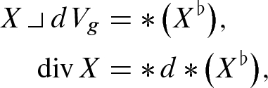
 is its volume form. If X is a smooth vector field on M, then
  is an
is an  -form. The exterior derivative of this
  -form is a smooth n-form, so it can be expressed as a smooth function multiplied by
  . That function is called the divergence of
  , and denoted by
  ; thus it is characterized by the following formula:
 on both sides of the equation, so
  is well defined, independently of the choice of orientation. In this way, we can define the divergence operator on any Riemannian manifold with or without boundary, by requiring that it satisfy (2.19) for any choice of orientation in a neighborhood of each point.
The most important application of the divergence operator is the divergence theorem, which you will be asked to prove in Problem 2-22.
 defined by
 . The main reason for choosing the negative sign is so that the operator will have nonnegative eigenvalues; see Problem 2-24. But the definition we give here is much more common in Riemannian geometry.)
The next proposition gives alternative formulas for these operators.
Proposition 2.46.
 be any smooth local coordinates on an open set
  . The coordinate representations of the divergence and Laplacian are as follows:

 is the determinant of the component matrix of g in these coordinates. On
  with the Euclidean metric and standard coordinates, these reduce to
Proof.
Problem 2-21. 
Lengths and Distances
Perhaps the most important tool that a Riemannian metric gives us is the ability to measure lengths of curves and distances between points. Throughout this section, (M, g) denotes a Riemannian manifold with or without boundary.
Without further qualification,
a curve in M always means a parametrized curve, that is, a continuous map  , where
  is some interval. Unless otherwise specified, we will not worry about whether the interval is bounded or unbounded, or whether it includes endpoints or not. To say that
  is a smooth curve is to say that it is smooth as a map from the manifold (with boundary) I to M. If I has one or two endpoints and M has empty boundary, then
  is smooth if and only if it extends to a smooth curve defined on some open interval containing I. (If
  , then smoothness of
  has to be interpreted as meaning that each coordinate representation of
  has a smooth extension to an open interval.) A curve segment is a curve whose domain is a compact interval.
A smooth curve  has a well-defined velocity
  for each
  . We say that
  is a regular curve if
  for
for  . This implies that
  is an immersion, so its image has no “corners” or “kinks.”
We wish to use curve segments as “measuring tapes" to define distances between points in a connected Riemannian manifold. Many aspects of the theory become technically much simpler if we work with a slightly larger class of curve segments instead of just the regular ones. We now describe the appropriate class of curves.
If ![$$[a, b]\subseteq \mathbb {R}$$](../images/56724_2_En_2_Chapter/56724_2_En_2_Chapter_TeX_IEq754.png) is a closed bounded interval, a partition of
is a closed bounded interval, a partition of ![$${\varvec{[a, b]}}$$](../images/56724_2_En_2_Chapter/56724_2_En_2_Chapter_TeX_IEq755.png) is a finite sequence
is a finite sequence  of real numbers such that
  . Each interval
 ![$$[a_{i-1}, a_i]$$](../images/56724_2_En_2_Chapter/56724_2_En_2_Chapter_TeX_IEq758.png) is called a subinterval of the partition. If M is a smooth manifold with or without boundary, a (continuous) curve segment
is called a subinterval of the partition. If M is a smooth manifold with or without boundary, a (continuous) curve segment ![$$\gamma :[a, b]\rightarrow M$$](../images/56724_2_En_2_Chapter/56724_2_En_2_Chapter_TeX_IEq759.png) is said to be piecewise regular if there exists a partition
is said to be piecewise regular if there exists a partition  of [a, b] such that
 ![$$\gamma |_{[a_{i-1}, a_{i}]}$$](../images/56724_2_En_2_Chapter/56724_2_En_2_Chapter_TeX_IEq761.png) is a regular curve segment (meaning it is smooth with nonvanishing velocity) for
is a regular curve segment (meaning it is smooth with nonvanishing velocity) for  . For brevity, we refer to a piecewise regular curve segment as an admissible curve, and any partition
  such that
 ![$$\gamma |_{[a_{i-1}, a_i]}$$](../images/56724_2_En_2_Chapter/56724_2_En_2_Chapter_TeX_IEq764.png) is smooth for each i an admissible partition for
is smooth for each i an admissible partition for  . (There are many admissible partitions for a given admissible curve, because we can always add more points to the partition.) It is also convenient to consider any map
  whose domain is a single real number to be an admissible curve.
 is an admissible curve and
  is an admissible partition for it. At each of the intermediate partition points
  , there are two one-sided velocity vectors, which we denote by

If  is a smooth curve, we define a reparametrization of
  to be a curve of the form
  , where
  is another interval and
  is a diffeomorphism. Because intervals are connected,
  is either strictly increasing or strictly decreasing on
  . We say that
  is a forward reparametrization if
  is increasing, and a backward reparametrization if it is decreasing.
For an admissible curve ![$$\gamma :[a, b]\rightarrow M$$](../images/56724_2_En_2_Chapter/56724_2_En_2_Chapter_TeX_IEq780.png) , we define a reparametrization of
, we define a reparametrization of  a little more broadly, as a curve of the form
  , where
 ![$$\varphi :[c,d]\rightarrow [a, b]$$](../images/56724_2_En_2_Chapter/56724_2_En_2_Chapter_TeX_IEq783.png) is a homeomorphism for which there is a partition
is a homeomorphism for which there is a partition  of [c, d] such that the restriction of
  to each subinterval
 ![$$[c_{i-1}, c_i]$$](../images/56724_2_En_2_Chapter/56724_2_En_2_Chapter_TeX_IEq786.png) is a diffeomorphism onto its image.
is a diffeomorphism onto its image.
![$$\gamma :[a, b]\rightarrow M$$](../images/56724_2_En_2_Chapter/56724_2_En_2_Chapter_TeX_IEq787.png) is an admissible curve, we define the length of
is an admissible curve, we define the length of  to be
to be

 is not smooth, so this integral is well defined.
Proposition 2.47
(Properties of Lengths). Suppose (M, g) is a Riemannian manifold with or without boundary, and ![$$\gamma :[a, b]\rightarrow M$$](../images/56724_2_En_2_Chapter/56724_2_En_2_Chapter_TeX_IEq791.png) is an admissible curve.
is an admissible curve.
- (a)Additivity of Length:If
 , then
 ![$$\begin{aligned} L_g(\gamma ) = L_g\big (\gamma \big |_{[a,c]}\big ) + L_g\big (\gamma \big |_{[c, b]}\big ). \end{aligned}$$](../images/56724_2_En_2_Chapter/56724_2_En_2_Chapter_TeX_Equ75.png)
- (b)
Parameter Independence: If
 is a reparametrization of
  , then
  .
. - (c)
Isometry Invariance: If (M, g) and
 are Riemannian manifolds (with or without boundary) and
  is a local isometry, then
  .
.
 Exercise 2.48. Prove Proposition 2.47.
![$$\gamma :[a, b]\rightarrow M$$](../images/56724_2_En_2_Chapter/56724_2_En_2_Chapter_TeX_IEq800.png) is an admissible curve. The arc-length function of
is an admissible curve. The arc-length function of  is the function
 ![$$s:[a, b]\rightarrow \mathbb {R}$$](../images/56724_2_En_2_Chapter/56724_2_En_2_Chapter_TeX_IEq802.png) defined by
defined by![$$\begin{aligned} s(t) = L_g\big (\gamma |_{[a, t]}\big ) = \int _a^t|\gamma '(u)|_g\, du. \end{aligned}$$](../images/56724_2_En_2_Chapter/56724_2_En_2_Chapter_TeX_Equ76.png)
 is, with derivative
  .
.For this reason, if  is any smooth curve (not necessarily a curve segment), we define the speed of
  at any time
  to be the scalar
  . We say that
  is a unit-speed curve if
  for all t, and a constant-speed curve if
  is constant. If
  is a piecewise smooth curve, we say that
  has unit speed if
  wherever
  is smooth.
If ![$$\gamma :[a, b]\rightarrow M$$](../images/56724_2_En_2_Chapter/56724_2_En_2_Chapter_TeX_IEq816.png) is a unit-speed admissible curve, then its arc-length function has the simple form
is a unit-speed admissible curve, then its arc-length function has the simple form  . If, in addition, its parameter interval is of the form [0, b] for some
  , then the arc-length function is
  . For this reason, a unit-speed admissible curve whose parameter interval is of the form [0, b] is said to be parametrized by arc length.
Proposition 2.49.
Suppose (M, g) is a Riemannian manifold with or without boundary.
- (a)
Every regular curve in M has a unit-speed forward reparametrization.
- (b)
Every admissible curve in M has a unique forward reparametrization by arc length.
Proof.
 is a regular curve. Choose an arbitrary
  , and define
  by
by
 , it follows that s is a strictly increasing local diffeomorphism, and thus maps I diffeomorphically onto an interval
  . If we let
  , then
  is a forward reparametrization of
  , and the chain rule gives
 is a unit-speed reparametrization of
  .
.![$$\gamma :[a, b]\rightarrow M$$](../images/56724_2_En_2_Chapter/56724_2_En_2_Chapter_TeX_IEq830.png) be an admissible curve. We prove the existence statement in part (b) by induction on the number of smooth segments in an admissible partition. If
be an admissible curve. We prove the existence statement in part (b) by induction on the number of smooth segments in an admissible partition. If  has only one smooth segment, then it is a regular curve segment, and (b) follows by applying (a) in the special case
 ![$$I=[a, b]$$](../images/56724_2_En_2_Chapter/56724_2_En_2_Chapter_TeX_IEq832.png) and choosing
and choosing  . Assuming that the result is true for admissible curves with k smooth segments, suppose
  has an admissible partition
  . The inductive hypothesis gives piecewise regular homeomorphisms
 ![$$\varphi :[0,c]\rightarrow [a, a_k]$$](../images/56724_2_En_2_Chapter/56724_2_En_2_Chapter_TeX_IEq836.png) and
and ![$$\psi :[0,d]\rightarrow [a_k, b]$$](../images/56724_2_En_2_Chapter/56724_2_En_2_Chapter_TeX_IEq837.png) such that
such that  is an arc-length reparametrization of
 ![$$\gamma |_{[a, a_k]}$$](../images/56724_2_En_2_Chapter/56724_2_En_2_Chapter_TeX_IEq839.png) and
and  is an arc-length reparametrization of
 ![$$\gamma |_{[a_k, b]}$$](../images/56724_2_En_2_Chapter/56724_2_En_2_Chapter_TeX_IEq841.png) . If we define
. If we define ![$$\tilde{\varphi }:[0,c+d]\rightarrow [a, b]$$](../images/56724_2_En_2_Chapter/56724_2_En_2_Chapter_TeX_IEq842.png) by
by
 is a reparametrization of
  by arc length.
 and
and  are both forward reparametrizations of
  by arc length. Since both have the same length, it follows that
  and
and  both have the same parameter domain [0, c], and thus both are piecewise regular homeomorphisms from [0, c] to [a, b]. If we define
 ![$$\eta = \varphi ^{-1}\circ \psi :[0,c]\rightarrow [0,c]$$](../images/56724_2_En_2_Chapter/56724_2_En_2_Chapter_TeX_IEq850.png) , then
, then  is a piecewise regular increasing homeomorphism satisfying
  . The fact that both
  and
and  are of unit speed implies the following equality for all
 ![$$s\in [0,c]$$](../images/56724_2_En_2_Chapter/56724_2_En_2_Chapter_TeX_IEq855.png) except the finitely many values at which
except the finitely many values at which  or
or  is not smooth:
 is continuous and
  , it follows that
  for all
 ![$$s\in [0,c]$$](../images/56724_2_En_2_Chapter/56724_2_En_2_Chapter_TeX_IEq861.png) , and thus
, and thus  .
. 
The Riemannian Distance Function
We are now in a position to introduce one of the most important concepts from classical geometry into the Riemannian setting: distances between points.
Suppose (M, g) is a connected Riemannian manifold with or without boundary. For each pair of points  , we define the Riemannian distance from
  to
to  , denoted by
  , to be the infimum of the lengths of all admissible curves from p to q. The following proposition guarantees that
  is a well-defined nonnegative real number for each
  .
.
Proposition 2.50.
If M is a connected smooth manifold (with or without boundary), then any two points of M can be joined by an admissible curve.
Proof.
Let  be arbitrary. Since a connected manifold is path-connected, p and q can be connected by a continuous path
 ![$$c:[a, b]\rightarrow M$$](../images/56724_2_En_2_Chapter/56724_2_En_2_Chapter_TeX_IEq872.png) . By compactness, there is a partition of [a, b] such that
. By compactness, there is a partition of [a, b] such that ![$$c\big ([a_{i-1}, a_i]\big )$$](../images/56724_2_En_2_Chapter/56724_2_En_2_Chapter_TeX_IEq873.png) is contained in a single smooth coordinate ball (or half-ball in case
is contained in a single smooth coordinate ball (or half-ball in case  ) for each i. Then we may replace each such curve segment by a straight-line path in coordinates, yielding an admissible curve
  between the same points (Fig. 2.2).
 denote the Riemannian distance from p to q, provided that p and q lie in the same connected component of M. (See also Problem 2-30.)
Any two points can be connected by an admissible curve
Proposition 2.51
(Isometry Invariance of the Riemannian Distance Function). Suppose (M, g) and  are connected Riemannian manifolds with or without boundary, and
  is an isometry. Then
  for all
  .
.
 Exercise 2.52. Prove the preceding proposition.
(Note that unlike lengths of curves, Riemannian distances are not necessarily preserved by local isometries; see Problem 2-31.)
We wish to show that the Riemannian distance function turns M into a metric space, whose metric topology is the same as its original manifold topology. To do so, we need the following lemmas.
Lemma 2.53.
 or
or  , and let
  denote the Euclidean metric on W. For every compact subset
  , there are positive constants c, C such that for all
  and all
  ,
,
Proof.
 by
by  for
for  and
and  . Let
. Let  be any compact subset, and define
  by
by
 with
with  , L is equal to the product set
  , which is compact. Since F is positive on L, there are positive constants c, C such that
 and
and  with
with  , we can write
  , where
  and
and  . Then
  , and it follows from the homogeneity of
  that
that
 . Arguing similarly in the other direction, we conclude that (2.21) holds for all
  and
and  .
. 
The next lemma shows how to transfer this result to Riemannian manifolds.
Lemma 2.54.
 be its Riemannian distance function. Suppose U is an open subset of M and
  . Then p has a coordinate neighborhood
  with the property that there are positive constants C, D satisfying the following inequalities:
- (a)
If
 , then
  , where
  is the Euclidean metric in the given coordinates on V.
 - (b)
If
 , then
  .
.
Proof.
 . Using these coordinates, we can identify W with an open subset of
  or
or  . Let K be a compact subset of W containing a neighborhood V of p, chosen as follows: If p is an interior point of M, let K be the closed Euclidean ball
  , with
  chosen small enough that
  , and let
  . If
. If  , let K be a closed half-ball
  with
with  chosen similarly, and let
  . Let
. Let  denote the Euclidean metric in these coordinates, and let c, C be constants satisfying (2.21). If
  is any admissible curve whose image lies entirely in V, it follows that
 . Letting
 ![$$\gamma :[a, b]\rightarrow V$$](../images/56724_2_En_2_Chapter/56724_2_En_2_Chapter_TeX_IEq932.png) be a parametrization of the line segment from p to q, we conclude from (2.22) that
be a parametrization of the line segment from p to q, we conclude from (2.22) that
 . If
. If ![$$\gamma :[a, b]\rightarrow M$$](../images/56724_2_En_2_Chapter/56724_2_En_2_Chapter_TeX_IEq934.png) is any admissible curve from p to q, let
is any admissible curve from p to q, let  denote the infimum of times
 ![$$t\in [a, b]$$](../images/56724_2_En_2_Chapter/56724_2_En_2_Chapter_TeX_IEq936.png) such that
such that  . It follows that
 ![$$\gamma \big ([a, t_0]\big )\subseteq K$$](../images/56724_2_En_2_Chapter/56724_2_En_2_Chapter_TeX_IEq938.png) and
and  by continuity (Fig. 2.3), so (2.22) implies
![$$\begin{aligned} L_{g}(\gamma ) \ge L_{g}\big (\gamma |_{[a, t_0]}\big )\ge c L_{{\bar{g}}}\big (\gamma |_{[a, t_0]}\big ) \ge c\, d_{{\bar{g}}}(p,\gamma (t_0)) =c\varepsilon . \end{aligned}$$](../images/56724_2_En_2_Chapter/56724_2_En_2_Chapter_TeX_Equ84.png)
 , we obtain (b) with
  .
. 


The triangle inequality
Theorem 2.55
(Riemannian Manifolds as Metric Spaces). Let (M, g) be a connected Riemannian manifold with or without boundary. With the distance function  , M is a metric space whose metric topology is the same as the given manifold topology.
Proof.
It is immediate from the definition of  that
that  and
and  . On the other hand, suppose
  are distinct. Let
  be an open set that contains p but not q, and choose a coordinate neighborhood V of p contained in U and satisfying the conclusion of Lemma 2.54. Then Lemma 2.54(b) shows that
  .
.
The triangle inequality follows from the fact that an admissible curve from p to q can be combined with one from q to r (possibly changing the starting time of the parametrization of the second) to yield one from p to r whose length is the sum of the lengths of the two given curves (Fig. 2.4). (This is one reason for defining distance using piecewise regular curves instead of just regular ones.) This completes the proof that  turns M into a metric space.
It remains to show that the metric topology is the same as the manifold topology. Suppose first that  is open in the manifold topology. For each
  , we can choose a coordinate neighborhood V of p contained in U with positive constants C, D satisfying the conclusions of Lemma 2.54. The contrapositive of part (b) of that lemma says
  , which means that the metric ball of radius D is contained in U. Thus U is open in the metric topology induced by
  .
.
On the other hand, suppose  is open in the metric topology. Given
  , choose
  such that the
  -metric ball of radius
  around p is contained in
  . Let V be any neighborhood of p that is open in the manifold topology and satisfies the conclusions of Lemma 2.54, with corresponding constants C, D. (We are not claiming that
  .) Choose
  small enough that
  . Lemma 2.54(a) shows that if q is a point of V such that
  , then
  , and thus q lies in the metric ball of radius
  about p, and hence in
  . Since the set
  is open in the given manifold topology, this shows that
  is also open in the manifold topology.
 is bounded if there is a constant C such that
  for all
  ; if this is the case, the diameter of
  is the smallest such constant:
 , not 2, since the Riemannian distance between antipodal points is
  . See Problem 6-2.)
Pseudo-Riemannian Metrics
From the point of view of geometry, Riemannian metrics are by far the most important structures that manifolds carry. However, there is a generalization of Riemannian metrics that has become especially important because of its application to physics.
 defined by
 is an isomorphism.
Lemma 2.56.
- (a)
q is nondegenerate.
- (b)
For every nonzero
 , there is some
  such that
  .
. - (c)
If
 in terms of some basis
  for
for  , then the matrix
  is invertible.
 Exercise 2.57. Prove the preceding lemma.
Every inner product is a nondegenerate symmetric bilinear form, as is every symmetric bilinear form that is negative definite (which is defined by obvious analogy with positive definite). But there are others that are neither positive definite nor negative definite, as we will see below.
We use the term scalar product to denote any nondegenerate symmetric bilinear form on a finite-dimensional vector space V, and reserve the term inner product for the special case of a positive definite scalar product. A scalar product space is a finite-dimensional vector space endowed with a scalar product. When convenient, we will often use a notation like  to denote a scalar product. We say that vectors
  are orthogonal if
  , just as in the case of an inner product. Given a vector
  , we define the norm of
  to be
to be  . Note that in the indefinite case, it is possible for a nonzero vector to be orthogonal to itself, and thus to have norm zero. Thus |v| is not technically a norm in the sense defined on page 47 below, but it is customary to call it “the norm of v” anyway.
 Exercise 2.58. Prove that the polarization identity (2.2) holds for every scalar product.
If  is any linear subspace, the set of vectors in V that are orthogonal to every vector in S is a linear subspace denoted by
  .
.
Lemma 2.59.
Suppose (V, q) is a finite-dimensional scalar product space, and  is a linear subspace.
- (a)
 .
. - (b)
 .
.
Proof.
Define a linear map  by
by  . Note that
  if and only if
  for all
  , so
, so  . If
. If  is arbitrary, there is a covector
  whose restriction to S is equal to
  . (For example, such a covector is easily constructed after choosing a basis for S and extending it to a basis for V.) Since
  is an isomorphism, there exists
  such that
  . It follows that
  , and therefore
  is surjective. By the rank–nullity theorem, the dimension of
  is equal to
  . This proves (a).
To prove (b), note that every  is orthogonal to every element of
  by definition, so
  . Because these finite-dimensional vector spaces have the same dimension by part (a), they are equal.
An ordered k-tuple  of elements of V is said to be orthonormal if
  for each i and
  for
for  , or equivalently, if
  for each i and j. We wish to prove that every scalar product space has an orthonormal basis. Note that the usual Gram–Schmidt algorithm does not always work in this situation, because the vectors that appear in the denominators in (2.5)–(2.6) might have vanishing norms. In order to get around this problem, we introduce the following definitions. If (V, q) is a finite-dimensional scalar product space, a subspace
  is said to be nondegenerate if the restriction of q to
  is nondegenerate. An ordered k-tuple of vectors
  in V is said to be nondegenerate if for each
  , the vectors
  span a nondegenerate j-dimensional subspace of V. For example, every orthonormal basis is nondegenerate.
Lemma 2.60.
 is a linear subspace. The following are equivalent:
- (a)
S is nondegenerate.
- (b)
 is nondegenerate.
 - (c)
 .
. - (d)
 .
.
 Exercise 2.61. Prove the preceding lemma.
Lemma 2.62
(Completion of Nondegenerate Bases). Suppose (V, q) is an n-dimensional scalar product space, and  is a nondegenerate k-tuple in V with
  . Then there exist vectors
  such that
  is a nondegenerate basis for V.
Proof.
Let  . Because
  ,
,  is a nontrivial subspace of V, and Lemma 2.60 shows that
  is nondegenerate and
  . By the nondegeneracy of
  , there must be a vector in
  with nonzero length, because otherwise the polarization identity would imply that all inner products of pairs of elements of S would be zero. If
  is any vector with nonzero length, then
  is easily seen to be a nondegenerate
  -tuple. Repeating this argument for
  completes the proof.
Proposition 2.63
(Gram–Schmidt Algorithm for Scalar Products). Suppose (V, q) is an n-dimensional scalar product space. If  is a nondegenerate basis for V, then there is an orthonormal basis
  with the property that
  for each
  .
.
Proof.
 is constructed recursively, starting with
  and noting that the assumption that
  spans a nondegenerate subspace ensures that
  . At the inductive step, assuming we have constructed
  , we first set
 is equal to
  , so this defines z as a nonzero element of V orthogonal to
  , and with the property that
  . If
. If  , then z is orthogonal to
  , contradicting the nondegeneracy assumption. Thus we can complete the inductive step by putting
  .
. 
Corollary 2.64.
 for
for  with respect to which q has the expression
 .
.Proof.
Let  be an orthonormal basis for V, and let
  be the dual basis for
  . A computation shows that q has a basis expression of the form (2.23), but perhaps with the positive and negative terms in a different order. Reordering the basis so that the positive terms come first, we obtain (2.23).
It turns out that the numbers r and s in (2.23) are independent of the choice of basis. The key to proving this is the following classical result from linear algebra.
Proposition 2.65
(Sylvester’s Law of Inertia). Suppose (V, q) is a finite-dimensional scalar product space. If q has the representation (2.23) in some basis, then the number r is the maximum dimension among all subspaces on which the restriction of q is positive definite, and thus r and s are independent of the choice of basis.
Proof.
Problem 2-33. 
The integer s in the expression (2.23) (the number of negative terms) is called the index of  , and the ordered pair (r, s) is called the signature of
  .
.
Now suppose M is a smooth manifold. A pseudo-Riemannian metric on  (called by some authors a semi-Riemannian metric) is a smooth symmetric 2-tensor field g that is nondegenerate at each point of M, and with the same signature everywhere. Every Riemannian metric is also a pseudo-Riemannian metric.
Proposition 2.66
(Orthonormal Frames for Pseudo-Riemannian Manifolds). Let (M, g) be a pseudo-Riemannian manifold. For each  , there exists a smooth orthonormal frame on a neighborhood of p in M.
 Exercise 2.67. Prove the preceding proposition.
 Exercise 2.68. Suppose
  and
and  are pseudo-Riemannian manifolds of signatures
  and
and  , respectively. Show that
  is a pseudo-Riemannian manifold of signature
  .
.
 , denoted by
  , to be the manifold
  , with standard coordinates denoted by
  , and with the pseudo-Riemannian metric
  defined by
 , so there is no significant difference.)
 is a Lorentz metric called the Minkowski metric, and the Lorentz manifold
  is called
  -dimensional Minkowski space. If we denote standard coordinates on
  by
by  , then the Minkowski metric is given by
 , the Minkowski metric is the fundamental invariant of Albert Einstein’s special theory of relativity, which can be expressed succinctly by saying that if gravity is ignored, then spacetime is accurately modeled by
  -dimensional Minkowski space, and the laws of physics have the same form in every coordinate system in which the Minkowski metric has the expression (2.25). The differing physical characteristics of “space” (the
  directions) and “time” (the
  direction) arise from the fact that they are subspaces on which the metric is positive definite and negative definite, respectively. The general theory of relativity includes gravitational effects by allowing the Lorentz metric to vary from point to point.
Many, but not all, results from the theory of Riemannian metrics apply equally well to pseudo-Riemannian metrics. Throughout this book, we will attempt to point out which results carry over directly to pseudo-Riemannian metrics, which ones can be adapted with minor modifications, and which ones do not carry over at all. As a rule of thumb, proofs that depend only on the nondegeneracy of the metric tensor, such as properties of the musical isomorphisms and existence and uniqueness of geodesics, work fine in the pseudo-Riemannian setting, while proofs that use positivity in an essential way, such as those involving lengths of curves, do not.
One notable result that does not carry over to the pseudo-Riemannian case is Proposition 2.4, about the existence of metrics. For example, the following result characterizes those manifolds that admit Lorentz metrics.
Theorem 2.69.
A smooth manifold M admits a Lorentz metric if and only if it admits a rank-1 tangent distribution (i.e., a rank-1 subbundle of TM).
Proof.
Problem 2-34. 
With some more sophisticated tools from algebraic topology, it can be shown that every noncompact connected smooth manifold admits a Lorentz metric, and a compact connected smooth manifold admits a Lorentz metric if and only if its Euler characteristic is zero (see [O’N83, p. 149]). It follows that no even-dimensional sphere admits a Lorentz metric, because  has Euler characteristic equal to 2.
For a thorough treatment of pseudo-Riemannian metrics from a mathematical point of view, see the excellent book [O’N83]; a more physical treatment can be found in [HE73].
Pseudo-Riemannian Submanifolds
The theory of submanifolds is only slightly more complicated in the pseudo-Riemannian case. If  is a pseudo-Riemannian manifold, a smooth submanifold
  is called a pseudo-Riemannian submanifold of
  if
if  is nondegenerate with constant signature. If this is the case, we always consider M to be endowed with the induced pseudo-Riemannian metric
  . In the special case in which
  is positive definite, M is called a Riemannian submanifold.
The nondegeneracy hypothesis is not automatically satisfied: for example, if  is the submanifold
  and
and  is inclusion, then the pullback tensor
  is identically zero on M.
For hypersurfaces (submanifolds of codimension 1), the nondegeneracy condition is easy to check. If  is a smooth submanifold and
  , then a vector
  is said to be normal to
  if
if  for all
  , just as in the Riemannian case. The space of all normal vectors at p is a subspace of
  denoted by
  .
.
Proposition 2.70.
Suppose  is a pseudo-Riemannian manifold of signature (r, s). Let M be a smooth hypersurface in
  , and let
  be the inclusion map. Then the pullback tensor field
  is nondegenerate if and only if
  for every
  and every nonzero normal vector
  . If
. If  for every nonzero normal vector to M, then M is a pseudo-Riemannian submanifold of signature
  ; and if
  for every such vector, then M is a pseudo-Riemannian submanifold of signature
  .
.
Proof.
Given  , Lemma 2.60 shows that
  is a nondegenerate subspace of
  if and only if the one-dimensional subspace
  is nondegenerate, which is the case if and only if every nonzero
  satisfies
  .
.
Now suppose  for every nonzero normal vector
  . Let
. Let  be arbitrary, and let
  be a nonzero element of
  . Writing
  , we can complete
  to a nondegenerate basis
  for
for  by Lemma 2.62, and then use the Gram–Schmidt algorithm to find an orthonormal basis
  for
for  such that
  . It follows that
  . If
. If  is the dual basis to
  , then
  has a basis representation of the form
  , with a total of r positive terms and s negative ones, and with a positive sign on the first term
  . Therefore,
  has signature
  . The argument for the case
  is similar.
If  is a pseudo-Riemannian manifold and
  , then the gradient of
  is defined as the smooth vector field
  just as in the Riemannian case.
Corollary 2.71.
Suppose  is a pseudo-Riemannian manifold of signature (r, s),
  , and
, and  for some
  . If
. If  everywhere on M, then M is an embedded pseudo-Riemannian submanifold of
  of signature
  ; and if
  everywhere on M, then M is an embedded pseudo-Riemannian submanifold of
  of signature
  . In either case,
  is everywhere normal to M.
Proof.
Problem 2-35. 
Proposition 2.72
(Pseudo-Riemannian Adapted Orthonormal Frames). Suppose  is a pseudo-Riemannian manifold, and
  is an embedded pseudo-Riemannian or Riemannian submanifold. For each
  , there exists a smooth orthonormal frame on a neighborhood of p in
  that is adapted to M.
Proof.
Write  and
and  , and let
  be arbitrary. Proposition 2.66 shows that there is a smooth orthonormal frame
  for M on some neighborhood of p in M. Then by Lemma 2.62, we can find vectors
  such that
  is a nondegenerate basis for
  . Now extend
  arbitrarily to smooth vector fields
  on a neighborhood of p in
  . By continuity, the ordered m-tuple
  will be a nondegenerate frame for
  in some (possibly smaller) neighborhood of p. Applying the Gram–Schmidt algorithm (Prop. 2.63) to this local frame yields a smooth local orthonormal frame
  for
for  with the property that
  restricts to a local orthonormal frame for M.
The next corollary is proved in the same way as Proposition 2.16.
Corollary 2.73
(Normal Bundle to a Pseudo-Riemannian Submanifold). Suppose  is a pseudo-Riemannian manifold, and
  is an embedded pseudo-Riemannian or Riemannian submanifold. The set of vectors normal to M is a smooth vector subbundle of
  , called the normal bundle to
  .
. 
Other Generalizations of Riemannian Metrics
Pseudo-Riemannian metrics are obtained by relaxing the positivity requirement for Riemannian metrics. In addition, there are other useful generalizations that result when we relax other requirements. In this section we touch briefly on two of those generalizations. We will not treat these anywhere else in the book, but it is useful to know the definitions.
Sub-Riemannian Metrics
The first generalization arises when we relax the requirement that the metric be defined on the whole tangent space.
A sub-Riemannian metric (also sometimes known as a singular Riemannian metric or Carnot–Carathéodory metric) on a smooth manifold M is a smooth fiber metric on a smooth tangent distribution  (i.e., a vector subbundle of TM). Since lengths make sense only for vectors in S, the only curves whose lengths can be measured are those whose velocity vectors lie everywhere in S. Therefore, one usually imposes some condition on S that guarantees that any two nearby points can be connected by such a curve. This is, in a sense, the opposite of the Frobenius integrability condition, which would restrict every such curve to lie in a single leaf of a foliation.
Sub-Riemannian metrics arise naturally in the study of the abstract models of real submanifolds of complex space  , called CR manifolds (short for Cauchy–Riemann manifolds). CR manifolds are real manifolds endowed with a tangent distribution
  whose fibers carry the structure of complex vector spaces (with an additional integrability condition that need not concern us here). In the model case of a submanifold
  , S is the set of vectors tangent to M that remain tangent after multiplication by
  in the ambient complex coordinates. If S is sufficiently far from being integrable, choosing a fiber metric on S results in a sub-Riemannian metric whose geometric properties closely reflect the complex-analytic properties of M as a subset of
  .
.
Another motivation for studying sub-Riemannian metrics arises from control theory. In this subject, one is given a manifold with a vector field depending on parameters called controls, with the goal being to vary the controls so as to obtain a solution curve with desired properties, often one that minimizes some function such as arc length. If the vector field is constrained to be everywhere tangent to a distribution S on the manifold (for example, in the case of a robot arm whose motion is restricted by the orientations of its hinges), then the function can often be modeled as a sub-Riemannian metric and optimal solutions modeled as sub-Riemannian geodesics.
A useful introduction to the geometry of sub-Riemannian metrics is provided in the article [Str86].
Finsler Metrics
Another important generalization arises from relaxing the requirement that norms of vectors be defined in terms of an inner product on each tangent space.
 , that satisfies
- (i)
Homogeneity:
 for
for  and
and  ;
; - (ii)
Positivity:
 for
for  , with equality if and only if
  ;
; - (iii)
Triangle Inequality:
 for
for  .
.
For example, the length function associated with an inner product is a norm.
Now suppose M is a smooth manifold. A Finsler metric on M is a continuous function  , smooth on the set of nonzero vectors, whose restriction to each tangent space
  is a norm. Again, the norm function associated with a Riemannian metric is a special case.
The inventor of Riemannian geometry himself, Bernhard Riemann, clearly envisaged an important role in n-dimensional geometry for what we now call Finsler metrics; he restricted his investigations to the “Riemannian” case purely for simplicity (see [Spi79, Vol. 2]). However, it was not until the late twentieth century that Finsler metrics began to be studied seriously from a geometric point of view.
The recent upsurge of interest in Finsler metrics has been motivated in part by the fact that two different Finsler metrics appear very naturally in the theory of several complex variables. For certain bounded open sets in  (the ones with smooth, strictly convex boundaries, for example), the Kobayashi metric and the Carathéodory metric are intrinsically defined, biholomorphically invariant Finsler metrics. Combining differential-geometric and complex-analytic methods has led to striking new insights into both the function theory and the geometry of such domains. We do not treat Finsler metrics further in this book, but you can consult one of the recent books on the subject
[AP94, BCS00, JP13].
(the ones with smooth, strictly convex boundaries, for example), the Kobayashi metric and the Carathéodory metric are intrinsically defined, biholomorphically invariant Finsler metrics. Combining differential-geometric and complex-analytic methods has led to striking new insights into both the function theory and the geometry of such domains. We do not treat Finsler metrics further in this book, but you can consult one of the recent books on the subject
[AP94, BCS00, JP13].
- 2-1.
Show that every Riemannian 1-manifold is flat. (Used on pp. 13, 193.)
- 2-2.
Suppose V and W are finite-dimensional real inner product spaces of the same dimension, and
 is any map (not assumed to be linear or even continuous) that preserves the origin and all distances:
  and
and  for all
  . Prove that F is a linear isometry. [Hint: First show that F preserves inner products, and then show that it is linear.] (Used on p. 187.)
 - 2-3.
Given a smooth embedded 1-dimensional submanifold
 as in Example 2.24(b), show that the surface of revolution
  with its induced metric is isometric to the warped product
  , where
  is the distance to the z-axis.
 - 2-4.
Let
 be the restriction of the standard coordinate function, and let
  denote the resulting warped product (see Example 2.24(c)). Define
  by
by  . Show that
  is an isometry between the warped product metric and the Euclidean metric on
  . (Used on p. 293.)
 - 2-5.
Prove parts (b) and (c) of Proposition 2.25 (properties of horizontal vector fields). (Used on p. 146.)
- 2-6.
Prove Theorem 2.28 (if
 is a surjective smooth submersion, and a group acts on
  isometrically, vertically, and transitively on fibers, then M inherits a unique Riemannian metric such that
  is a Riemannian submersion).
 - 2-7.
For
 , the set
  of k-dimensional linear subspaces of
  is called a Grassmann manifold or Grassmannian. The group
  acts transitively on
  in an obvious way, and
  has a unique smooth manifold structure making this action smooth (see [LeeSM, Example 21.21]).
- (a)
Let
 denote the set of orthonormal ordered k-tuples of vectors in
  . By arranging the vectors in k columns, we can view
  as a subset of the vector space
  of all
  real matrices. Prove that
  is a smooth submanifold of
  of dimension
  , called a Stiefel manifold. [Hint: Consider the map
  given by
  .]
.] - (b)
Show that the map
 that sends a k-tuple to its span is a surjective smooth submersion.
 - (c)
Give
 the Riemannian metric induced from the Euclidean metric on
  . Show that the right action of
  on
on  by matrix multiplication on the right is isometric, vertical, and transitive on fibers of
  , and thus there is a unique metric on
  such that
  is a Riemannian submersion. [Hint: It might help to note that the Euclidean inner product on
  can be written in the form
  .]
.](Used on p. 82.)
- (a)
- 2-8.
Prove that the action of
 on
on  defined in Example 2.35 is smooth, free, proper, and isometric, and therefore the open Möbius band inherits a flat Riemannian metric such that the quotient map is a Riemannian covering.
 - 2-9.
Prove Proposition 2.37 (the gradient is orthogonal to regular level sets).
- 2-10.
Suppose (M, g) is a Riemannian manifold,
 , and
, and  is a nowhere-vanishing vector field. Prove that
  if and only if
  and X is orthogonal to the level sets of f at all regular points of f. (Used on pp. 161, 180.)
 - 2-11.
Prove Proposition 2.40 (inner products on tensor bundles).
- 2-12.
Prove Proposition 2.41 (existence and uniqueness of the Riemannian volume form).
- 2-13.
Prove Proposition 2.43 (characterizing the volume form of a Riemannian hypersurface). [Hint: To prove (2.17), use an adapted orthonormal frame.]
- 2-14.
Suppose
 and (M, g) are compact connected Riemannian manifolds, and
  is a k-sheeted Riemannian covering. Prove that
  . (Used on p. 363.)
 - 2-15.Suppose
 and
and  are oriented Riemannian manifolds of dimensions
  and
and  , respectively. Let
  be a smooth function, and let
  be the corresponding warped product metric on
  . Prove that the Riemannian volume form of g is given by where f,
 , and
, and  are understood to be pulled back to
  by the projection maps. (Used on p. 295.)
 - 2-16.Let (M, g) be a Riemannian n-manifold. Show that for each
 , there is a unique
fiber metric
, there is a unique
fiber metric  on the bundle
  that satisfies whenever
 (2.26)
 are covectors at a point
  . [Hint: Define the inner product locally by declaring the set of k-covectors to be an orthonormal basis for
 whenever
  is a local orthonormal coframe for
  , and then prove that the resulting inner product satisfies (2.26) and is independent of the choice of frame.]
 - 2-17.
Because we regard the bundle
 of k-forms as a subbundle of the bundle
  of covariant k-tensors, we have two inner products to choose from on k-forms: the one defined in Problem 2-16, and the restriction of the tensor inner product defined in Proposition 2.40. For this problem, we use the notation
  to denote the inner product of Problem 2-16, and
  to denote the restriction of the tensor inner product.
- (a)Using the convention for the wedge product that we use in this book (see p. 400), prove that

- (b)Show that if the Alt convention is used for the wedge product (p. 401), the formula becomes

- (a)
- 2-18.
Let (M, g) be an oriented Riemannian n-manifold.
- (a)For each
 show that there is a unique smooth bundle homomorphism
  , called the
Hodge star operator
, satisfying for all smooth k-forms
, called the
Hodge star operator
, satisfying for all smooth k-forms
 ,
,  , where
  is the inner product on k-forms defined in Problem 2-16. (For
  interpret the inner product as ordinary multiplication.) [Hint: First prove uniqueness, and then define
  locally by setting in terms of an orthonormal coframe
 , where the indices
  are chosen such that
  is some permutation of
  .]
.] - (b)
Show that
 is given by
  .
. - (c)
Show that
 if
if  is a k-form.
- (a)
- 2-19.
Regard
 as a Riemannian manifold with the Euclidean metric and the standard orientation, and let
  denote the Hodge star operator defined in Problem 2-18.
- (a)
Calculate
 for
for  .
. - (b)
Calculate
 in the case
  .
.
- (a)
- 2-20.
Let M be an oriented Riemannian 4-manifold. A 2-form
 on M is said to be self-dual if
  and anti-self-dual if
  .
.- (a)
Show that every 2-form
 on M can be written uniquely as a sum of a self-dual form and an anti-self-dual form.
 - (b)
On
 with the Euclidean metric, determine the self-dual and anti-self-dual forms in standard coordinates.
- (a)
- 2-21.
Prove Proposition 2.46 (the coordinate formulas for the divergence and the Laplacian).
- 2-22.
Suppose (M, g) is a compact Riemannian manifold with boundary.
- (a)Prove the following divergence theorem for
 : where N is the outward unit normal to
 and
and  is the induced metric on
  . [Hint: Prove it first in the case that M is orientable, and then apply that case to the orientation covering of M (Prop. B.18).]
 - (b)Show that the divergence operator satisfies the following product rule for
 and
and  : and deduce the following “integration by parts” formula:
 What does this say when M is a compact interval in
 ? (Used on p. 149.)
- (a)
- 2-23.
Let (M, g) be a compact Riemannian manifold with or without boundary. A function
 is said to be harmonic if
  , where
  is the Laplacian defined on page 32.
- (a)Prove Green’s identities:where N is the outward unit normal vector field on

 and
and  is the induced metric on
  .
. - (b)
Show that if M is connected,
 , and u, v are harmonic functions on M whose restrictions to
  agree, then
  .
. - (c)
Show that if M is connected and
 , then the only harmonic functions on M are the constants, and every smooth function u satisfies
  .
.(Used on pp. 149, 223.)
- (a)
- 2-24.
Let (M, g) be a compact Riemannian manifold (without boundary). A real number
 is called an
eigenvalue of
is called an
eigenvalue of
 if there exists a smooth function u on M, not identically zero, such that
  . In this case, u is called an
eigenfunction
corresponding to
. In this case, u is called an
eigenfunction
corresponding to  .
.- (a)
Prove that 0 is an eigenvalue of M, and that all other eigenvalues are strictly positive.
- (b)
Show that if u and v are eigenfunctions corresponding to distinct eigenvalues, then
 .
.(Used on p. 149.)
- (a)
- 2-25.
Let (M, g) be a compact connected Riemannian n-manifold with nonempty boundary. A number
 is called a
Dirichlet eigenvalue for
is called a
Dirichlet eigenvalue for
 if there exists a smooth real-valued function u on M, not identically zero, such that
  and
and  . Similarly,
  is called a
Neumann eigenvalue
if there exists such a u satisfying
is called a
Neumann eigenvalue
if there exists such a u satisfying  and
and  , where N is the outward unit normal.
- (a)
Show that every Dirichlet eigenvalue is strictly positive.
- (b)
Show that 0 is a Neumann eigenvalue, and all other Neumann eigenvalues are strictly positive.
- (a)
- 2-26.
Dirichlet’s Principle:Suppose (M, g) is a compact connected Riemannian n-manifold with nonempty boundary. Prove that a function
 is harmonic if and only if it minimizes
  among all smooth functions with the same boundary values. [Hint: For any function
  that vanishes on
  expand
  and use Problem 2-22.]
 - 2-27.
Suppose (M, g) is an oriented Riemannian 3-manifold.
- (a)Define
 by
by  . Show that
  is a smooth bundle isomorphism, and thus we can define the curl of a vector field
  by
by 
- (b)Show that the following diagram commutes:where
 (2.27)
 , and use this to prove that
  for every
  , and
, and  for every
  .
. - (c)
Compute the formula for the curl in standard coordinates on
 with the Euclidean metric.
- (a)
- 2-28.
- 2-29.
Let (M, g) be a compact oriented Riemannian n-manifold. For
 , define a map
  by
by  , where
  is the
Hodge star operator defined in Problem 2-18. Extend this definition to 0-forms by defining
is the
Hodge star operator defined in Problem 2-18. Extend this definition to 0-forms by defining  for
for  .
.- (a)
Show that
 .
. - (b)Show that the formuladefines an inner product on

 for each k, where
  is the inner product on forms defined in Problem 2-16.
 - (c)
Show that
 for all
  and
and  .
.
- (a)
- 2-30.
Suppose (M, g) is a (not necessarily connected) Riemannian manifold. Show that there is a distance function d on M that induces the given topology and restricts to the Riemannian distance on each component of M. (Used on p. 187.)
- 2-31.
Suppose (M, g) and
 are connected Riemannian manifolds, and
  is a local isometry. Show that
  for all
  . Give an example to show that equality need not hold. (Used on p. 37.)
 - 2-32.Let (M, g) be a Riemannian manifold and
![$$\gamma :[a, b]\rightarrow M$$](../images/56724_2_En_2_Chapter/56724_2_En_2_Chapter_TeX_IEq1393.png) a smooth curve segment. For each continuous function
a smooth curve segment. For each continuous function ![$$f:[a, b]\rightarrow \mathbb {R}$$](../images/56724_2_En_2_Chapter/56724_2_En_2_Chapter_TeX_IEq1394.png) , we define the integral of
, we define the integral of  with respect to arc length, denoted by
  , by
, by 
- (a)Show that
 is independent of parametrization in the following sense: if
 ![$$\varphi :[c,d]\rightarrow [a, b]$$](../images/56724_2_En_2_Chapter/56724_2_En_2_Chapter_TeX_IEq1398.png) is a diffeomorphism, then where
is a diffeomorphism, then where
 and
and  .
. - (b)Suppose now that
 is a smooth embedding, so that
 ![$$C= \gamma ([a, b])$$](../images/56724_2_En_2_Chapter/56724_2_En_2_Chapter_TeX_IEq1402.png) is an embedded submanifold with boundary in M. Show that where
is an embedded submanifold with boundary in M. Show that where
 is the Riemannian volume element on C associated with the induced metric and the orientation determined by
  .
.(Used on p. 273.)
- (a)
- 2-33.
Prove Proposition 2.65 (Sylvester’s law of inertia).
- 2-34.
Prove Theorem 2.69 (existence of Lorentz metrics), as follows.
- (a)
For sufficiency, assume that
 is a 1-dimensional distribution, and choose any Riemannian metric g on M. Show that locally it is possible to choose a g-orthonormal frame
  and dual coframe
  such that
  spans D; and then show that the Lorentz metric
  is independent of the choice of frame.
 - (b)
To prove necessity, suppose that g is a Lorentz metric on M, and let
 be any Riemannian metric. Show that for each
  , there are exactly two
  -unit vectors
  ,
,  on which the function
  takes its minimum among all unit vectors in
  , and use Lagrange multipliers to conclude that there exists a number
  such that
  for all
  . You may use the following standard result from perturbation theory: if U is an open subset of
  and
and  is a smooth matrix-valued function such that A(x) is symmetric and has exactly one negative eigenvalue for each
  , then there exist smooth functions
  and
and  such that
  for all
  .
.
- (a)
- 2-35.
Prove Corollary 2.71 (about level sets in pseudo-Riemannian manifolds). (Used on p. 63.)