In this chapter, we begin our study of the local invariants of Riemannian metrics. Starting with the question whether all Riemannian metrics are locally isometric, we are led to a definition of the Riemannian curvature tensor as a measure of the failure of second covariant derivatives to commute. Then we prove the main result of this chapter: a Riemannian manifold has zero curvature if and only if it is flat, or locally isometric to Euclidean space. Next, we derive the basic symmetries of the curvature tensor, and introduce the Ricci, scalar, and Weyl curvature tensors. At the end of the chapter, we explore how the curvature can be used to detect conformal flatness. As you will see, the results of this chapter apply essentially unchanged to pseudo-Riemannian metrics.
Local Invariants
For any geometric structure defined on smooth manifolds, it is of great interest to address the local equivalence question: Are all examples of the structure locally equivalent to each other (under an appropriate notion of local equivalence)?
Nonvanishing vector fields: Every nonvanishing vector field can be written as
 in suitable local coordinates, so they are all locally equivalent.
Riemannian metrics on a 1-manifold: Problem 2-1 shows that every Riemannian 1-manifold is locally isometric to
 with its Euclidean metric.
Symplectic forms: A symplectic form on a smooth manifold M is a closed 2-form
 that is nondegenerate at each
  , meaning that
  for all
  only if
  . By the theorem of Darboux [LeeSM, Thm. 22.13], every symplectic form can be written in suitable coordinates as
  . Thus all symplectic forms on 2n-manifolds are locally equivalent.
On the other hand, Problem 5-5 showed that the round 2-sphere and the Euclidean plane are not locally isometric.
The most important technique for proving that two geometric structures are not locally equivalent is to find local invariants , which are quantities that must be preserved by local equivalences. In order to address the general problem of local equivalence of Riemannian or pseudo-Riemannian metrics, we will define a local invariant for all such metrics called curvature. Initially, its definition will have nothing to do with the curvature of curves described in Chapter 1, but later we will see that the two concepts are intimately related.
 must have the same property locally.
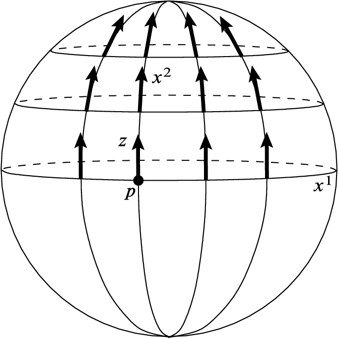
Result of parallel transport along the  -axis and the
  -coordinate lines
 : working in any smooth local coordinates
  centered at p, first parallel transport z along the
  -axis, and then parallel transport the resulting vectors along the coordinate lines parallel to the
  -axis (Fig. 7.1). The result is a vector field Z that, by construction, is parallel along every
  -coordinate line and along the
  -axis. The question is whether this vector field is parallel along
  -coordinate lines other than the
  -axis, or in other words, whether
  . Observe that
  vanishes when
  . If we could show that
 , because the zero vector field is the unique parallel transport of zero along the
  -curves. If we knew that
 everywhere by construction. Indeed, on
  with the Euclidean metric, direct computation shows that
 is equal to the same thing, because ordinary second partial derivatives commute. However, (7.2) might not hold for an arbitrary Riemannian metric; indeed, it is precisely the noncommutativity of such second covariant derivatives that forces this construction to fail on the sphere. Lurking behind this noncommutativity is the fact that the sphere is “curved.”
 when X, Y, and Z are smooth vector fields. On
  with the Euclidean connection, we just showed that this always vanishes if
  and
and  ; however, for arbitrary vector fields this may no longer be true. In fact, in
  with the Euclidean connection we have
 . The difference between these two expressions is
 ![$$\big (XY\big (Z^k\big )-YX\big (Z^k\big )\big )\partial _{k} = \bar{\nabla }_{[X, Y]}Z$$](../images/56724_2_En_7_Chapter/56724_2_En_7_Chapter_TeX_IEq34.png) . Therefore, the following relation holds for all vector fields X, Y, Z defined on an open subset of
. Therefore, the following relation holds for all vector fields X, Y, Z defined on an open subset of  :
:![$$\begin{aligned} \bar{\nabla }_X\bar{\nabla }_Y Z - \bar{\nabla }_Y\bar{\nabla }_X Z = \bar{\nabla }_{[X, Y]}Z. \end{aligned}$$](../images/56724_2_En_7_Chapter/56724_2_En_7_Chapter_TeX_Equ62.png)
 with its Euclidean metric. Similarly, a pseudo-Riemannian manifold is flat if it is locally isometric to a pseudo-Euclidean space. The computation above leads to the following simple necessary condition for a Riemannian or pseudo-Riemannian manifold to be flat. We say that a connection
  on a smooth manifold M satisfies the flatness criterion if whenever X, Y, Z are smooth vector fields defined on an open subset of M, the following identity holds:
![$$\begin{aligned} \nabla _X\nabla _Y Z - \nabla _Y\nabla _X Z = \nabla _{[X, Y]}Z. \end{aligned}$$](../images/56724_2_En_7_Chapter/56724_2_En_7_Chapter_TeX_Equ3.png)
Example 7.1.
The metric on the n-torus induced by the embedding in  given in Example 2.21 is flat, because each point has a coordinate neighborhood in which the metric is Euclidean. //
Proposition 7.2.
If (M, g) is a flat Riemannian or pseudo-Riemannian manifold, then its Levi-Civita connection satisfies the flatness criterion.
Proof.
We just showed that the Euclidean connection on  satisfies (7.3). By naturality, the Levi-Civita connection on every manifold that is locally isometric to a Euclidean or pseudo-Euclidean space must also satisfy the same identity.
The Curvature Tensor
 by
by
![$$\begin{aligned} R(X,Y)Z = \nabla _X\nabla _Y Z - \nabla _Y\nabla _X Z - \nabla _{[X, Y]}Z. \end{aligned}$$](../images/56724_2_En_7_Chapter/56724_2_En_7_Chapter_TeX_Equ63.png)
Proposition 7.3.
The map R defined above is multilinear over  , and thus defines a (1, 3)-tensor field on M.
Proof.
 . For
. For  ,
,![$$\begin{aligned} \begin{aligned} R(X,fY)Z&= \nabla _{X}\nabla _{fY} Z - \nabla _{fY}\nabla _{X} Z - \nabla _{[X,fY]}Z\\&= \nabla _{X}(f\nabla _YZ) - f\nabla _{Y}\nabla _{X} Z- \nabla _{f[X,Y] + (Xf)Y}Z\\&= (Xf) \nabla _YZ + f\nabla _{X}\nabla _YZ - f\nabla _{Y}\nabla _{X} Z\\&\quad - f\nabla _{[X,Y]}Z - (Xf)\nabla _{Y}Z\\&= fR(X, Y)Z. \end{aligned} \end{aligned}$$](../images/56724_2_En_7_Chapter/56724_2_En_7_Chapter_TeX_Equ64.png)
 in X, because
  from the definition. The remaining case to be checked is linearity over
  in Z; this is left to Problem 7-1.
By the tensor characterization lemma (Lemma B.6), the fact that R is multilinear over  implies that it is a (1, 3)-tensor field.
Thanks to this proposition, for each pair of vector fields  , the map
  given by
  is a smooth bundle endomorphism of TM, called the
curvature endomorphism determined by X and Y
. The tensor field R itself is called the
(
Riemann) curvature endomorphism or the (1, 3)-curvature tensor. (Some authors call it simply the curvature tensor, but we reserve that name instead for another closely related tensor field, defined below.)
is a smooth bundle endomorphism of TM, called the
curvature endomorphism determined by X and Y
. The tensor field R itself is called the
(
Riemann) curvature endomorphism or the (1, 3)-curvature tensor. (Some authors call it simply the curvature tensor, but we reserve that name instead for another closely related tensor field, defined below.)
 as
as
 are defined by
Proposition 7.4.

Proof.
Problem 7-2. 
Importantly for our purposes, the curvature endomorphism also measures the failure of second covariant derivatives along families of curves to commute. Given a smooth one-parameter family of curves  , recall from Chapter 6 that the velocity fields
  and
and  are smooth vector fields along
  .
.
Proposition 7.5.
 is a smooth one-parameter family of curves in M. Then for every smooth vector field V along
  ,
,
Proof.
 , we can choose smooth coordinates
  defined on a neighborhood of
  and write


 is extendible,
 is also extendible,
 and
and  and subtracting, we find that the first terms cancel, and we get

 (also denoted by
  by some authors) obtained from the (1, 3)-curvature tensor R by lowering its last index. Its action on vector fields is given by

 . Thus (7.4) yields
The next proposition gives one reason for our interest in the curvature tensor.
Proposition 7.6.
The curvature tensor is a local isometry invariant: if (M, g) and  are Riemannian or pseudo-Riemannian manifolds and
  is a local isometry, then
  .
.
 Exercise 7.7. Prove Proposition 7.6.
Flat Manifolds
To give a qualitative geometric interpretation to the curvature tensor, we will show that it is precisely the obstruction to being locally isometric to Euclidean (or pseudo-Euclidean) space. (In Chapter 8, after we have developed more machinery, we will be able to give a far more detailed quantitative interpretation.) The crux of the proof is the following lemma.
Lemma 7.8.
Suppose M is a smooth manifold, and  is any connection on M satisfying the flatness criterion. Given
  and any vector
  , there exists a parallel vector field V on a neighborhood of p such that
  .
.
Proof.
Let  and
and  be arbitrary, and let
  be any smooth coordinates for M centered at p. By shrinking the coordinate neighborhood if necessary, we may assume that the image of the coordinate map is an open cube
  . We use the coordinate map to identify the coordinate domain with
  .
.
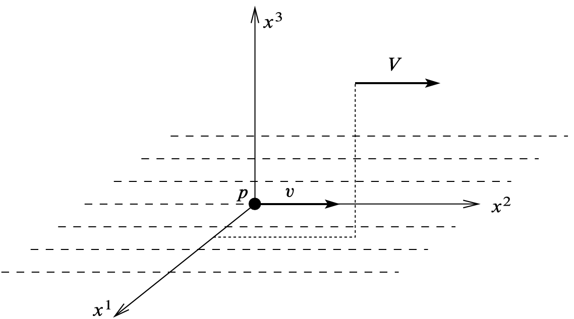
Begin by parallel transporting v along the  -axis; then from each point on the
  -axis, parallel transport along the coordinate line parallel to the
  -axis; then successively parallel transport along coordinate lines parallel to the
  through
  -axes (Fig. 7.2). The result is a vector field V defined in
  . The fact that V is smooth follows from an inductive application of the theorem concerning smooth dependence of solutions to linear ODEs on initial conditions (Thm. 4.31); the details are left as an exercise.
 is linear over
  in X, to show that V is parallel, it suffices to show that
  for each
  . By construction,
  on the
  -axis,
  on the
  -plane, and in general
  on the slice
  defined by
  . We will prove the following fact by induction on k:
 , this is true by construction, and for
  , it means that V is parallel on the whole cube
  . So assume that (7.9) holds for some k. By construction,
  on all of
  , and for
  , the inductive hypothesis shows that
  on the hyperplane
  .
.![$$[\partial _{k+1},\partial _i]=0$$](../images/56724_2_En_7_Chapter/56724_2_En_7_Chapter_TeX_IEq114.png) , the flatness criterion gives
, the flatness criterion gives
 is parallel along the
  -curves starting on
  . Since
  vanishes on
  and the zero vector field is the unique parallel transport of zero, we conclude that
  is zero on each
  -curve. Since every point of
  is on one of these curves, it follows that
  on all of
  . This completes the inductive step to show that V is parallel.
Proof of Lemma 7.8
 Exercise 7.9. Prove that the vector field V constructed in the preceding proof is smooth.
Theorem 7.10.
A Riemannian or pseudo-Riemannian manifold is flat if and only if its curvature tensor vanishes identically.
Proof.
One direction is immediate: Proposition 7.2 showed that the Levi-Civita connection of a flat metric satisfies the flatness criterion, so its curvature endomorphism is identically zero, which implies that the curvature tensor is also zero.
Now suppose (M, g) has vanishing curvature tensor. This means that the curvature endomorphism vanishes as well, so the Levi-Civita connection satisfies the flatness criterion. We begin by showing that g shares one important property with Euclidean and pseudo-Euclidean metrics: it admits a parallel orthonormal frame in a neighborhood of each point.
Let  , and choose an orthonormal basis
  for
for  . In the pseudo-Riemannian case, we may assume that the basis is in standard order (with positive entries before negative ones in the matrix
  ). Lemma 7.8 shows that there exist parallel vector fields
  on a neighborhood U of p such that
  for each
  . Because parallel transport preserves inner products, the vector fields
  are orthonormal (and hence linearly independent) in all of U.
![$$\begin{aligned}{}[E_i, E_j] = \nabla _{E_i}E_j - \nabla _{E_j}E_i = 0. \end{aligned}$$](../images/56724_2_En_7_Chapter/56724_2_En_7_Chapter_TeX_Equ76.png)
 form a commuting orthonormal frame on U. The canonical form theorem for commuting vector fields (Prop. A.48) shows that there are coordinates
  on a (possibly smaller) neighborhood of p such that
  for
for  . In any such coordinates,
  , so the map
  is an isometry from a neighborhood of p to an open subset of the appropriate Euclidean or pseudo-Euclidean space.
Using similar ideas, we can give a more precise interpretation of the meaning of the curvature tensor: it is a measure of the extent to which parallel transport around a small rectangle fails to be the identity map.
Theorem 7.11.
 be a smooth one-parameter family of curves; and let
  ,
,  , and
, and  . For any
  , let
, let  denote parallel transport along the curve
  from time
  to time
  , and let
  denote parallel transport along the curve
  from time
  to time
  . (See Fig. 7.3.) Then for every
  ,
,

The curvature endomorphism and parallel transport around a closed loop
Proof.
 by first parallel transporting z along the curve
  , and then for each t, parallel transporting Z(0, t) along the curve
  . The resulting vector field along
  is smooth by another application of Theorem 4.31; and by construction, it satisfies
  for all
  , and
, and  for all
  . Proposition 7.5 shows that
 is equal to the limit on the right-hand side of (7.10).


Symmetries of the Curvature Tensor
The curvature tensor on a Riemannian or pseudo-Riemannian manifold has a number of symmetries besides the obvious skew-symmetry in its first two arguments.
Proposition 7.12
- (a)
 .
. - (b)
 .
. - (c)
 .
. - (d)
 .
.
 is also zero. Finally, it is useful to record the form of these symmetries in terms of components with respect to any basis:
 - (
 )
)  .
.- (
 )
)  .
.- (
 )
)  .
.- (
 )
)  .
.
 . To prove (b), it suffices to show that
  for all Y, for then (b) follows from the expansion of
  . Using compatibility with the metric, we have
![$$\begin{aligned} WX|Y|^2&= W(2\langle \nabla _XY, Y\rangle ) = 2\langle \nabla _W\nabla _XY, Y\rangle + 2\langle \nabla _XY,\nabla _WY\rangle ;\\ XW|Y|^2&= X(2\langle \nabla _WY, Y\rangle ) = 2\langle \nabla _X\nabla _WY, Y\rangle + 2\langle \nabla _WY,\nabla _XY\rangle ;\\ [W, X]|Y|^2&= 2\langle \nabla _{[W,X]}Y, Y\rangle . \end{aligned}$$](../images/56724_2_En_7_Chapter/56724_2_En_7_Chapter_TeX_Equ79.png)
 and
and  cancel on the right-hand side, giving
![$$\begin{aligned} 0&= 2\langle \nabla _W\nabla _XY, Y\rangle -2\langle \nabla _X\nabla _WY, Y\rangle -2\langle \nabla _{[W,X]}Y, Y\rangle \\&= 2\langle R(W,X)Y, Y\rangle \\&= 2 Rm (W,X,Y, Y). \end{aligned}$$](../images/56724_2_En_7_Chapter/56724_2_En_7_Chapter_TeX_Equ80.png)
 , this will follow immediately from
![$$\begin{aligned} (&\nabla _W\nabla _XY-\nabla _X\nabla _WY-\nabla _{[W,X]}Y)\\&+(\nabla _X\nabla _YW-\nabla _Y\nabla _XW-\nabla _{[X,Y]}W) \\&+(\nabla _Y\nabla _WX-\nabla _W\nabla _YX-\nabla _{[Y,W]}X)\\&\quad = \nabla _W(\nabla _XY-\nabla _YX) + \nabla _X(\nabla _YW-\nabla _WY) + \nabla _Y(\nabla _WX-\nabla _XW) \\&\qquad -\nabla _{[W,X]}Y-\nabla _{[X,Y]}W-\nabla _{[Y,W]}X\\&\quad = \nabla _W[X,Y] + \nabla _X[Y,W] + \nabla _Y[W,X] \\&\qquad -\nabla _{[W,X]}Y-\nabla _{[X,Y]}W-\nabla _{[Y,W]}X\\&\quad = [W,[X,Y]] + [X,[Y,W]] + [Y,[W, X]]. \end{aligned}$$](../images/56724_2_En_7_Chapter/56724_2_En_7_Chapter_TeX_Equ82.png)

 , which is equivalent to (c).
There is one more identity that is satisfied by the covariant derivatives of the curvature tensor on every Riemannian manifold. Classically, it was called the second Bianchi identity , but modern authors tend to use the more informative name differential Bianchi identity .
Proposition 7.13


Proof.
 , (7.14) is equivalent to
Let p be an arbitrary point, let  be normal coordinates centered at p, and let X, Y, Z, V, W be arbitrary coordinate basis vector fields. These vectors satisfy two properties that simplify our computations enormously: (1) their commutators vanish identically, since
 ![$$[\partial _i,\partial _j]\equiv 0$$](../images/56724_2_En_7_Chapter/56724_2_En_7_Chapter_TeX_IEq195.png) ; and (2) their covariant derivatives vanish at p, since
; and (2) their covariant derivatives vanish at p, since  (Prop. 5.24(d)).
![$$\begin{aligned} (\nabla _W Rm ) (Z,V,X,Y)&= \nabla _W \big ( Rm (Z,V,X,Y) \big )\\&= \nabla _W \langle R(Z,V)X,\ Y \rangle \\&= \nabla _W \langle \nabla _Z \nabla _V X - \nabla _V \nabla _Z X - \nabla _{[Z, V]} X, \ Y \rangle \\&=\langle \nabla _W \nabla _Z\nabla _V X - \nabla _W \nabla _V\nabla _Z X ,\ Y \rangle . \end{aligned}$$](../images/56724_2_En_7_Chapter/56724_2_En_7_Chapter_TeX_Equ84.png)

 at p.
at p. 
The Ricci Identities
 is a smooth
  -tensor field, and for vector fields X and Y, the notation
  denotes
  . Given vector fields X and Y, let
  denote the dual map to R(X, Y), defined by
Theorem 7.14

 is a smooth 1-form,

 and vector fields
  . In terms of any local frame, the component versions of these formulas read


Proof.
![$$\begin{aligned} \begin{aligned} \nabla ^2_{X, Y}B - \nabla ^2_{Y,X}B&= \nabla _X \nabla _Y B - \nabla _{(\nabla _X Y)}B - \nabla _Y\nabla _X B + \nabla _{(\nabla _Y X)}B\\&= \nabla _X \nabla _Y B - \nabla _Y\nabla _X B - \nabla _{[X, Y]}B, \end{aligned} \end{aligned}$$](../images/56724_2_En_7_Chapter/56724_2_En_7_Chapter_TeX_Equ23.png)
 is a vector field, so (7.17) follows directly from the definition of the curvature endomorphism.

![$$\begin{aligned} \big (\nabla _{[X,Y]}\beta \big ) (Z) = [X,Y](\beta (Z)) - \beta \big ( \nabla _{[X, Y]}Z\big ). \end{aligned}$$](../images/56724_2_En_7_Chapter/56724_2_En_7_Chapter_TeX_Equ26.png)
![$$\begin{aligned} \big ( \nabla _X\nabla _Y \beta - \nabla _Y\nabla _X\beta - \nabla _{[X,Y]}\beta \big ) (Z)&= - \beta \big (\nabla _X\nabla _Y Z - \nabla _Y\nabla _X Z - \nabla _{[X,Y]}Z\big )\\&= - \beta \big (R(X, Y)Z\big ), \end{aligned}$$](../images/56724_2_En_7_Chapter/56724_2_En_7_Chapter_TeX_Equ87.png)
 on an arbitrary tensor product:
![$$\begin{aligned} \big (\nabla ^2_{X, Y}&- \nabla ^2_{Y,X}\big )(F\otimes G)\\&= \big (\nabla _X\nabla _Y - \nabla _Y\nabla _X - \nabla _{[X,Y]}\big )(F\otimes G)\\&= \nabla _X\nabla _Y F\otimes G + \nabla _Y F\otimes \nabla _X G + \nabla _X F \otimes \nabla _Y G + F \otimes \nabla _X\nabla _Y G\\&\quad - \nabla _Y\nabla _X F\otimes G - \nabla _X F\otimes \nabla _Y G - \nabla _Y F \otimes \nabla _X G - F \otimes \nabla _Y\nabla _X G\\&\quad - \nabla _{[X,Y]} F\otimes G - F\otimes \nabla _{[X, Y]} G\\&= \big (\nabla ^2_{X, Y} F - \nabla ^2_{Y, X}F \big )\otimes G + F \otimes \big (\nabla ^2_{X, Y}G - \nabla ^2_{Y, X}G\big ). \end{aligned}$$](../images/56724_2_En_7_Chapter/56724_2_En_7_Chapter_TeX_Equ88.png)
 and 1-forms
  ,
,


Ricci and Scalar Curvatures
 (or often Ric in the literature), which is the covariant 2-tensor field defined as the trace of the curvature endomorphism on its first and last indices. Thus for vector fields X, Y,
 are usually denoted by
  , so that

Lemma 7.15.

 Exercise 7.16. Prove Lemma 7.15, using the symmetries of the curvature tensor.

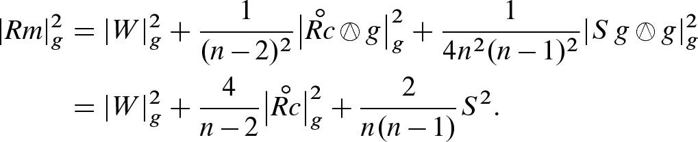
Proposition 7.17.
 , and the Ricci tensor decomposes orthogonally as

Remark.
The statement about norms, and others like it that we will prove below, works only in the Riemannian case because of the additional absolute value signs required to compute norms in the pseudo-Riemannian case. The pseudo-Riemannian analogue would be  , but this is not as useful.
Proof.

 that
that  and (7.27) holds. The fact that the decomposition is orthogonal follows easily from the fact that for every symmetric 2-tensor h, we have
 . Finally, (7.28) follows from (7.27) and the fact that
  .
. 


 by the result of Problem 5-13. The exterior covariant derivative can be generalized to other types of tensors as well, but this is the only case we need.)
Proposition 7.18


Proof.
Start with the component form (7.15) of the differential Bianchi identity, raise the index m, and then contract on the indices i, m to obtain (7.32). (Note that covariant differentiation commutes with contraction by Proposition 4.15 and with the musical isomorphisms by Proposition 5.17, so it does not matter whether the indices that are raised and contracted come before or after the semicolon.) Then do the same with the indices j, k and simplify to obtain (7.33). The coordinate-free formulas (7.30) and (7.31) follow by expanding everything out in components. 
It is important to note that if the sign convention chosen for the curvature tensor is the opposite of ours, then the Ricci tensor must be defined as the trace of  on the first and third (or second and fourth) indices. (The trace on the first two or last two indices is always zero by antisymmetry.) The definition is chosen so that the Ricci and scalar curvatures have the same meaning for everyone, regardless of the conventions chosen for the full curvature tensor. So, for example, if a manifold is said to have positive scalar curvature, there is no ambiguity as to what is meant.

 is constant; just assuming that the Ricci tensor is a function times the metric is sufficient.
Proposition 7.19
(Schur’s Lemma). Suppose (M, g) is a connected Riemannian or pseudo-Riemannian manifold of dimension  whose Ricci tensor satisfies
  for some smooth real-valued function f. Then f is constant and g is an Einstein metric.
Proof.
 shows that
  , so the traceless Ricci tensor is identically zero. It follows that
  . Because the covariant derivative of the metric is zero, this implies the following equation in any coordinate chart:

 , this implies
  . But
. But  is the component of
  , so connectedness of M implies that S is constant and thus so is f.
Corollary 7.20.
If (M, g) is a connected Riemannian or pseudo-Riemannian manifold of dimension  , then g is Einstein if and only if
  .
.
Proof.
Suppose first that g is an Einstein metric with  . Taking traces of both sides, we find that
  , and therefore
  . Conversely, if
  , Schur’s lemma implies that g is Einstein.
By an argument analogous to those of Chapter 6, Hilbert showed (see [Bes87, Thm. 4.21]) that Einstein metrics are critical points for the total scalar curvature functional  on the space of all metrics on M with fixed volume. Thus Einstein metrics can be viewed as “optimal” metrics in a certain sense, and as such they form an appealing higher-dimensional analogue of locally homogeneous metrics on 2-manifolds, with which one might hope to prove some sort of generalization of the uniformization theorem (Thm. 3.22). Although the statement of such a theorem cannot be as elegant as that of its 2-dimensional ancestor because there are known examples of smooth, compact manifolds that admit no Einstein metrics [Bes87, Chap. 6], there is still a reasonable hope that “most” higher-dimensional manifolds (in some sense) admit Einstein metrics. This is an active field of current research; see [Bes87] for a sweeping survey of Einstein metrics.

In the special case  , (7.35) reduces to the
vacuum Einstein field equation
, (7.35) reduces to the
vacuum Einstein field equation
 . Taking traces of both sides and recalling that
  , we obtain
  , which implies
  . Therefore, the vacuum Einstein equation is equivalent to
  , which means that g is a (pseudo-Riemannian) Einstein metric in the mathematical sense of the word. (At one point in the development of the theory, Einstein considered adding a term
  to the left-hand side of (7.35), where
  is a constant that he called the cosmological constant. With this modification the vacuum Einstein field equation would be exactly the same as the mathematicians’ Einstein equation (7.34). Einstein soon decided that the cosmological constant was a mistake on physical grounds; however, researchers in general relativity have recently begun to believe that a theory with a nonzero cosmological constant might in fact have physical relevance.)
Other than these special cases and the obvious formal similarity between (7.35) and (7.34), there is no direct connection between the physicists’ version of the Einstein equation and the mathematicians’ version. The mathematical interest in Riemannian Einstein metrics stems more from their potential applications to uniformization in higher dimensions than from their relation to physics.
Another approach to generalizing the uniformization theorem to higher dimensions is to search for metrics of constant scalar curvature. These are also critical points of thetotal scalar curvature functional, but only with respect to variations of the metric with fixed volume within a given conformal equivalence class. Thus it makes sense to ask whether, given a metric g on a manifold M, there exists a metric  conformal to g that has constant scalar curvature. This is called the Yamabe problem, because it was first posed in 1960 by Hidehiko Yamabe, who claimed to have proved that the answer is always yes when M is compact. Yamabe’s proof was later found to be in error, and it was two dozen years before the proof was finally completed by Richard Schoen; see [LP87] for an expository account of Schoen’s solution. When M is noncompact, the issues are much subtler, and much current research is focused on determining exactly which conformal classes contain metrics of constant scalar curvature.
The Weyl Tensor
As noted above, the Ricci and scalar curvatures contain only part of the information encoded into the curvature tensor. In this section, we introduce a tensor field called the Weyl tensor, which encodes all the rest.
 denote the vector space of all covariant 4-tensors T on V that have the symmetries of the (0, 4) Riemann curvature tensor:
- (a)
 .
. - (b)
 .
. - (c)
 .
. - (d)
 .
.
 is called an algebraic curvature tensor on V.
Proposition 7.21.

Proof.
 denote the linear subspace of
  consisting of tensors satisfying properties (a)–(c), and let
  denote the space of symmetric bilinear forms on the vector space
  of alternating contravariant 2-tensors on V. Define a map
  as follows:
 satisfies (a)–(c), so
  , and that
  is a linear map. In fact, it is an isomorphism, which we prove by constructing an inverse for it. Choose a basis
  for V, so the collection
  is a basis for
  . Define a map
  by setting
 and
and  , and extending by bilinearity. A straightforward computation shows that
  is an inverse for
  .
.
 and the dimension of the space of symmetric bilinear forms on a vector space of dimension m is
  .
. defined by
 is equal to the kernel of
  . In fact,
  is equal to the restriction to
  of the operator
  defined by (B.9): thanks to the symmetries (a)–(c), the 24 terms in the definition of
  can be arranged in three groups of eight in such a way that all the terms in each group reduce to one of the terms in the definition of
  . Thus the image of
  is contained in
  . In fact, the image is all of
  : every
  satisfies (a)–(c) and thus lies in
  , and
, and  for each such tensor.

Let us now assume that our vector space V is endowed with a (not necessarily positive definite) scalar product  . Let
. Let  denote the trace operation (with respect to g) on the first and last indices (so that, for example,
  ). It is natural to wonder whether this operator is surjective and what its kernel is, as a way of asking how much of the information contained in the Riemann curvature tensor is captured by the Ricci tensor. One way to try to answer the question is to attempt to construct a right inverse for the trace operator—a linear map
  such that
  for all
  .
.
 , we define a covariant 4-tensor
  , called the Kulkarni–Nomizu product of h and k, by the following formula:
 are
are
Lemma 7.22
(Properties of the Kulkarni–Nomizu Product). Let V be an n-dimensional vector space endowed with a scalar product g, let h and k be symmetric 2-tensors on V, let T be an algebraic curvature tensor on V, and let  denote the trace on the first and last indices.
- (a)
 is an algebraic curvature tensor.
 - (b)
 .
. - (c)
 .
. - (d)
 .
. - (e)
 .
. - (f)
In case g is positive definite,
 .
.
Proof.
It is evident from the definition that  has three of the four symmetries of an algebraic curvature tensor: it is antisymmetric in its first two arguments and also in its last two, and its value is unchanged when the first two and last two arguments are interchanged. Thus to prove (a), only the algebraic Bianchi identity needs to be checked. This is a straightforward computation: when
  is written three times with the arguments w, x, y cyclically permuted and the three expressions are added together, all the terms cancel due to the symmetry of h and k.

 .
.The proofs of (e) and (f) are left to Problem 7-9. 
Here is the primary application of the Kulkarni–Nomizu product.
Proposition 7.23.
 , and define a linear map
  by
by
 , and its image is the orthogonal complement of the kernel of
  in
in  .
.Proof.
The fact that G is a right inverse is a straightforward computation based on the definition and Lemma 7.22(c, d). This implies that G is injective and  is surjective, so the dimension of
  is equal to the codimension of
  , which in turn is equal to the dimension of
  . If
. If  is an algebraic curvature tensor such that
  , then Lemma 7.22(e) shows that
  , so it follows by dimensionality that
  .
. 


Proposition 7.24.
For every Riemannian or pseudo-Riemannian manifold (M, g) of dimension  , the trace of the Weyl tensor is zero, and
  is the orthogonal decomposition of
  corresponding to
  .
.
Proof.
This follows immediately from Proposition 7.23 and the fact that  .
. 
These results lead to some important simplifications in low dimensions.
Corollary 7.25.
Let V be an n-dimensional real vector space.
- (a)
If
 or
or  , then
  .
. - (b)
If
 , then
  is 1-dimensional, spanned by
  .
. - (c)
If
 , then
  is 6-dimensional, and
  is an isomorphism.
Proof.
The dimensional results follow immediately from Proposition 7.21. In the case  , Lemma 7.22(d) shows that
  , which implies that
  is nonzero and therefore spans the 1-dimensional space
  .
.
Now consider  . Proposition 7.23 shows that
  is the identity, which means that
  is injective. On the other hand, Proposition 7.21 shows that
  , so G is also surjective.
The next corollary shows that the entire curvature tensor is determined by the Ricci tensor in dimension 3.
Corollary 7.26
 ). On every Riemannian or pseudo-Riemannian manifold (M, g) of dimension 3, the Weyl tensor is zero, and the Riemann curvature tensor is determined by the Ricci tensor via the formula
Proof.
Corollary 7.25 shows that  is an isomorphism in dimension 3. Since
  is the identity, it follows that
  is also an isomorphism. Because
  is always zero by Proposition 7.24, it follows that W is always zero. Formula (7.39) then follows from the definition of the Weyl tensor.
In dimension 2, the definitions of the Weyl and Schouten tensors do not make sense; but we have the following analogous result instead.
Corollary 7.27
 ). On every Riemannian or pseudo-Riemannian manifold (M, g) of dimension 2, the Riemann and Ricci tensors are determined by the scalar curvature as follows:
Proof.
In dimension 2, it follows from Corollary 7.25(b) that there is some scalar function f such that  . Taking traces, we find from Lemma 7.22(d) that
  , and then
  . The results follow by substituting
  back into these equations.
Although the traceless Ricci tensor is always zero on a 2-manifold, this does not imply that S is constant, since the proof of Schur’s lemma fails in dimension 2.Einstein metrics in dimension 2 are simply those with constant scalar curvature.
Returning now to dimensions greater than 2, we can use (7.27) to further decompose the Schouten tensor into a part determined by the traceless Ricci tensor and a purely scalar part. The next proposition is the analogue of Proposition 7.17 for the full curvature tensor.
Proposition 7.28
 . Then the (0, 4)-curvature tensor of g has the following orthogonal decomposition:

Curvatures of Conformally Related Metrics
Recall that two Riemannian or pseudo-Riemannian metrics on the same manifold are said to be conformal to each other if one is a positive function times the other. For example, we have seen that the round metrics and the hyperbolic metrics are all conformal to Euclidean metrics, at least locally.
If g and  are conformal metrics on a smooth manifold M, there is no reason to expect that the curvature tensors of g and
  should be closely related to each other. But it is a remarkable fact that the Weyl tensor has a very simple transformation law under conformal changes of metric. In this section, we derive that law.
First we need to determine how the Levi-Civita connection changes when a metric is changed conformally. Given conformal metrics g and  , we can always write
  for some smooth real-valued function f.
Proposition 7.29
 be any metric conformal to g. If
  and
and  denote the Levi-Civita connections of g and
  , respectively, then

 is the ith component of
  .
.Proof.
Formula (7.43) is a straightforward computation using formula (5.10) for the Christoffel symbols in coordinates, and then (7.42) follows by expanding everything in coordinates and using (7.43). 
This result leads to transformation laws for the various curvature tensors.
Theorem 7.30
 , and
, and  . In the Riemannian case, the curvature tensors of
  (represented with tildes) are related to those of g by the following formulas:


 is the Laplacian of f defined in Chapter 2. If in addition
  , then


 replaced by
  .
.Proof.
 in normal coordinates for g centered at p, so that the equations
  ,
,  , and
, and  hold at p. This has the following consequences at p:


 .
. 
The next corollary begins to explain the geometric significance of the Weyl tensor. Recall that a Riemannian manifold is said to be locally conformally flat if every point has a neighborhood that is conformally equivalent to an open subset of Euclidean space. Similarly, a pseudo-Riemannian manifold is locally conformally flat if every point has a neighborhood conformally equivalent to an open set in a pseudo-Euclidean space.
Corollary 7.31.
Suppose (M, g) is a Riemannian or pseudo-Riemannian manifold of dimension  . If g is locally conformally flat, then its Weyl tensor vanishes identically.
Proof.
Suppose (M, g) is locally conformally flat. Then for each  there exist a neighborhood U and an embedding
  such that
  pulls back a flat (Riemannian or pseudo-Riemannian) metric on
  to a metric of the form
  . This implies that
  has zero Weyl tensor, because its entire curvature tensor is zero. By virtue of (7.48), the Weyl tensor of g is also zero.
 . This is the 3-tensor field whose expression in terms of any local frame is
Proposition 7.32.
 , and let W and C denote its Weyl and Cotton tensors, respectively. Then
 .
.Proof.
 and using the component form of the first contracted Bianchi identity (7.32), we obtain
 and
and  . To simplify the other two terms, we use the definition of the Schouten tensor and the second contracted Bianchi identity (7.33) to obtain that
 . When we insert these expressions into (7.51) and simplify, we find that the terms involving derivatives of the Ricci and scalar curvatures combine to yield

Corollary 7.33.
Suppose (M, g) is a Riemannian or pseudo-Riemannian manifold. If  and the Weyl tensor vanishes identically, then so does the Cotton tensor.
The next proposition expresses another important feature of the Cotton tensor.
Proposition 7.34
(Conformal Invariance of the Cotton Tensor in Dimension  ). Suppose
(M, g) is a Riemannian or pseudo-Riemannian 3-manifold, and
). Suppose
(M, g) is a Riemannian or pseudo-Riemannian 3-manifold, and  for some
  . If C and
  denote the Cotton tensors of g and
  , respectively, then
  .
.
Proof.
Problem 7-10. 
Corollary 7.35.
If (M, g) is a locally conformally flat 3-manifold, then the Cotton tensor of g vanishes identically.
 Exercise 7.36. Prove this corollary.
The real significance of the Weyl and Cotton tensors is explained by the following important theorem.
Theorem 7.37
(Weyl–Schouten). Suppose (M, g) is a Riemannian or pseudo-Riemannian manifold of dimension  .
.
- (a)
If
 , then (M, g) is locally conformally flat if and only if its Weyl tensor is identically zero.
 - (b)
If
 , then (M, g) is locally conformally flat if and only if its Cotton tensor is identically zero.
Proof.
The necessity of each condition was proved in Corollaries 7.31 and 7.35. To prove sufficiency, suppose (M, g) satisfies the hypothesis appropriate to its dimension; then it follows from Corollaries 7.26 and 7.33 that the Weyl and Cotton tensors of g are both identically zero. Every metric  conformal to g also has zero Weyl tensor, and therefore its curvature tensor is
  . We will show that in a neighborhood of each point, the function f can be chosen to make
  , which implies that
  and therefore
  is flat.
 if and only if
 , where A is the map from 1-tensors to symmetric 2-tensors given by

 that satisfies
  . In any local coordinates, if we write
  , this becomes an overdetermined system of first-order partial differential equations for the n unknown functions
  . (A system of differential equations is said to be overdetermined if there are more equations than unknown functions.) If
  is a solution to
  on an open subset of M, then the Ricci identity (7.21) shows that
  satisfies
 has a smooth solution in a neighborhood of each point, provided that for every smooth covector field
  , the covariant derivatives of
  satisfy
  when
when  is substituted for
  wherever it appears.
 wherever it appears, subtract
  , and use the relation
  . After extensive cancellations, we obtain
 to
to  in a neighborhood of each point.
Because  is symmetric in i and j, it follows that the ordinary derivatives
  are also symmetric, and thus
  is a closed 1-form. By the Poincaré lemma, in some (possibly smaller) neighborhood of each point, there is a smooth function f such that
  ; this f is the function we seek.
Here is the lemma that was used in the proof of the preceding theorem.
Lemma 7.38.

 is a smooth map satisfying the following compatibility condition: for any smooth covector field
  , the 3-tensor field
  satisfies the following identity when
  is substituted for
  wherever it appears:
 and every covector
  , there is a smooth solution to (7.56) on a neighborhood of p satisfying
  .
.Proof.
 be given. In smooth local coordinates
  on a neighborhood of p, (7.56) is equivalent to the overdetermined system

 arbitrary, provided that
 , after substituting
  in place of
  , are symmetric in the indices j, k. Because
  , this substitution is equivalent to substituting
  for
for  wherever it occurs. After expanding the hypothesis (7.57) in terms of Christoffel symbols, we find after some manipulation that it reduces to (7.58).
Because all Riemannian 1-manifolds are flat, the only nontrivial case that is not addressed by the Weyl–Schouten theorem is that of dimension 2. Smooth coordinates that provide a conformal equivalence between an open subset of a Riemannian or pseudo-Riemannian 2-manifold and an open subset of  are called isothermal coordinates, and it is a fact that such coordinates always exist locally. For the Riemannian case, there are various proofs available, all of which involve more machinery from partial differential equations and complex analysis than we have at our disposal; see [Che55] for a reasonably elementary proof. For the pseudo-Riemannian case, see Problem 7-15. Thus every Riemannian or pseudo-Riemannian 2-manifold is locally conformally flat.
Problems
- 7-1.
Complete the proof of Proposition 7.3 by showing that
 for all smooth vector fields X, Y, Z and smooth real-valued functions f.
 - 7-2.
Prove Proposition 7.4 (the formula for the curvature tensor in coordinates).
- 7-3.
Show that the curvature tensor of a Riemannian locally symmetric space is parallel:
 . (Used on pp. 297, 351.)
 - 7-4.Let M be a Riemannian or pseudo-Riemannian manifold, and let
 be normal coordinates centered at
  . Show that the following holds at p:
- 7-5.Let
 be the Levi-Civita connection on a Riemannian or pseudo-Riemannian manifold (M, g), and let
  be its connection 1-forms with respect to a local frame
  (Problem 4-14). Define a matrix of 2-forms
  , called the curvature 2-forms, by where
 is the coframe dual to
  . Show that the curvature 2-forms satisfy
Cartan’s second structure equation
: [Hint: Expand
. Show that the curvature 2-forms satisfy
Cartan’s second structure equation
: [Hint: Expand
 in terms of
  and
and  .]
.] - 7-6.Suppose
 and
and  are Riemannian manifolds, and
  is endowed with the product metric
  as in (2.12). Show that the Riemann curvature, Ricci curvature, and scalar curvature of g are given by the following formulas: where
 ,
,  , and
, and  are the Riemann, Ricci, and scalar curvatures of
  , and
, and  is the projection. (Used on pp. 257, 261.)
 - 7-7.
- 7-8.
Lichnerowicz’s Theorem: Suppose (M, g) is a compact Riemannian n-manifold, and there is a positive constant
 such that the Ricci tensor of g satisfies
  for all tangent vectors v. If
  is any positive eigenvalue of M, then
  . [Hint: Use Probs. 2-23(c), 5-15, and 7-7.]
 - 7-9.
Prove parts (e) and (f) of Lemma 7.22 (properties of the Kulkarni–Nomizu product).
- 7-10.
Prove Proposition 7.34 (conformal invariance of the Cotton tensor in dimension 3).
- 7-11.Let (M, g) be a Riemannian manifold of dimension
 . Define the
conformal Laplacian
. Define the
conformal Laplacian
 by the formula where
 is the Laplace–Beltrami operator of g and S is its scalar curvature. Prove that if
  for some
  , and
, and  denotes the conformal Laplacian with respect to
  , then for every
  , Conclude that a metric
 conformal to g has constant scalar curvature
  if and only if it can be expressed in the form
  , where
  is a smooth positive solution to the Yamabe equation:
  (7.59)
 - 7-12.Let M be a smooth manifold and let
 be any connection on TM. We can define the curvature endomorphism of
  by the same formula as in the Riemannian case:
 ![$$R(X,Y)Z = \nabla _X\nabla _Y Z - \nabla _Y\nabla _X Z - \nabla _{[X, Y]}Z$$](../images/56724_2_En_7_Chapter/56724_2_En_7_Chapter_TeX_IEq514.png) . Then
. Then  is said to be a
flat connection
if
is said to be a
flat connection
if  . Prove that the following are equivalent:
- (a)
 is flat.
 - (b)
For every point
 , there exists a parallel local frame defined on a neighborhood of p.
 - (c)
For all
 , parallel transport along an admissible curve segment
  from p to q depends only on the path-homotopy class of
  .
. - (d)
Parallel transport around any sufficiently small closed curve is the identity; that is, for every
 , there exists a neighborhood U of p such that if
 ![$$\gamma :[a, b]\mathrel {\rightarrow }U$$](../images/56724_2_En_7_Chapter/56724_2_En_7_Chapter_TeX_IEq523.png) is an admissible curve in U starting and ending at p, then
is an admissible curve in U starting and ending at p, then  is the identity map.
- (a)
- 7-13.Let G be a Lie group with a bi-invariant metric g. Show that the following formula holds whenever X, Y, Z are left-invariant vector fields on G:(See Problem 5-8.)
![$$\begin{aligned} R(X, Y)Z = \frac{1}{4} [Z,[X, Y]]. \end{aligned}$$](../images/56724_2_En_7_Chapter/56724_2_En_7_Chapter_TeX_Equ124.png)
- 7-14.Suppose
 is a
Riemannian submersion. Using the notation and results of Problem 5-6, prove O’Neill’s formula: (Used on p. 258.)
is a
Riemannian submersion. Using the notation and results of Problem 5-6, prove O’Neill’s formula: (Used on p. 258.)![$$\begin{aligned} Rm(W,X,Y, Z)\circ&\pi = \widetilde{Rm}\big ({\smash [t]{\widetilde{W}}},{{\tilde{X}}},{{\tilde{Y}}},{{\tilde{Z}}}\big ) - \frac{1}{2} \Big \langle \big [{\smash [t]{\widetilde{W}}},{{\tilde{X}}}\big ]^V, \big [{{\tilde{Y}}},{{\tilde{Z}}}\big ]^V\Big \rangle \\&\;\; - \frac{1}{4} \Big \langle \big [{\smash [t]{\widetilde{W}}},{{\tilde{Y}}}\big ]^V, \big [{{\tilde{X}}},{{\tilde{Z}}}\big ]^V\Big \rangle + \frac{1}{4} \Big \langle \big [{\smash [t]{\widetilde{W}}},{{\tilde{Z}}}\big ]^V, \big [{{\tilde{X}}},{{\tilde{Y}}}\big ]^V\Big \rangle . \end{aligned}$$](../images/56724_2_En_7_Chapter/56724_2_En_7_Chapter_TeX_Equ125.png)
- 7-15.
Suppose (M, g) is a 2-dimensional pseudo-Riemannian manifold of signature (1, 1), and
 .
.- (a)
Show that there is a smooth local frame
 in a neighborhood of p such that
  .
. - (b)
Show that there are smooth coordinates (x, y) in a neighborhood of p such that
 for some smooth, positive real-valued function f. [Hint: Use Prop. A.45 to show that there exist coordinates (t, u) in which
  , and coordinates (v, w) in which
  , and set
  ,
,  .]
.] - (c)
Show that (M, g) is locally conformally flat.
- (a)

