We have seen that in perfectly competitive markets, many small price-taking firms earn zero economic profit in the long run, prices to consumers are low, and output is at the socially efficient level. We have also seen that in monopoly markets, one large firm maintains positive economic profit in the long run, prices are high, and output is reduced so that deadweight loss is created. Both of these outcomes are uncommon in the real world because the basic assumptions of these two models are very strict. Markets in the real world operate somewhere in between perfect competition and monopoly, and we investigate these imperfectly competitive markets in this chapter.
After completing this chapter, the student should be able to:
1. Describe the key assumptions of monopolistic competition and oligopoly.
2. Draw a graph that shows the monopolistically competitive firm maximizing short-run profit and a graph that shows the long-run outcome.
3. Describe the key assumptions of oligopoly.
4. Understand the basics of strategic games between two players, including the concepts of dominant strategies, the prisoners’ dilemma, and Nash equilibria.
In many communities, markets such as the retail clothing market and the restaurant market can be described as good approximations of monopolistic competition. Let’s look at the key assumptions of this model to see how this might be the case.
• Many sellers exist in the market.
• Each seller produces a good that is similar, but not identical, to the goods produced by its competitors. This is known as product differentiation.
• Very few barriers to entry exist.
Before we dive straight into the theory and the graphs, consider some of the restaurants in a community. The Mexican, Italian, and Chinese restaurants all produce dine-in meals for customers, but the menus are clearly distinct. In fact, the dining experience, which is an important part of the meal, is also differentiated by the décor, the music, and the members of the service staff. Because of the deliberate product differentiation each restaurant has created for its product, each has a small degree of price-setting ability. In other words, they are not price takers like firms in perfect competition, and if demand for their product is strong enough, they might earn positive economic profits.
However, as we will see, because of the low barriers to entry, those profits will exist only in the short run. In the long run, as new firms enter, each firm will find it more difficult to attract enough demand for its product to maintain the profits. In addition, we will find that the entry of new firms stops when firms are earning breakeven profits, as in the perfectly competitive model. Let’s see how this works.
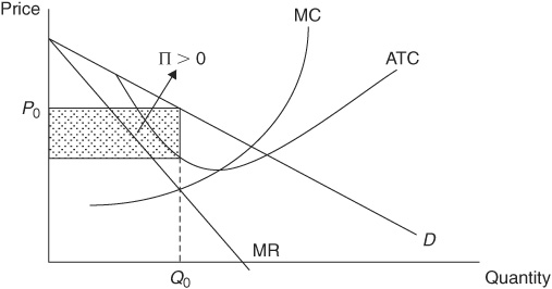
Suppose that Suzy Q’s BBQ is one of many dining options in town. Because it sells a product that is differentiated from that of all the other restaurants, Suzy Q’s is not a price-taking firm. The demand curve for its product is downward-sloping, and thus, like a monopoly firm, it has a marginal revenue curve that is below the demand curve and twice as steep. However, because we know that there are many close substitutes for its product, the demand for its product is probably quite elastic. Like all firms, Suzy Q’s maximizes profit by finding the output level where marginal revenue equals marginal cost and then finding the corresponding price from the demand curve. Suzy’s short-run situation is shown in Figure 9-1.
FIGURE 9-1 • Suzy Q’s Short-Run Situation
At the moment, the demand for Suzy’s BBQ is strong enough so that she earns positive economic profit, shown by the rectangle in Figure 9-1, and the model of monopolistic competition predicts that all the restaurants in this town will be experiencing similar profits of their own. However, what happens when entrepreneurs outside of the restaurant market notice that profits are being made? To answer that, we need to explore the long-run adjustment process.
Since there are minimal barriers to entry, new restaurateurs will open up to compete for customers and profits in the market. When they do, the demand for existing restaurants, like Suzy Q’s, will start to decrease and probably become even more elastic. When the demand and marginal revenue curves shift to the left, the rectangle of profit from Figure 9-1 will begin to shrink. When firms like Suzy Q’s are breaking even, the entry of new firms will cease. We can see the long-run outcome in Figure 9-2. The only way for firms to break even is when the output (QLR) is such that price (PLR) is equal to average total cost. When the demand for Suzy’s is downward-sloping, this will appear as a point of tangency between the demand curve and the average total cost curve.
FIGURE 9-2 • Suzy Q’s Long-Run Outcome
So what do we make of this outcome? It tells us that monopolistically competitive markets will be extremely competitive and that firms will find it very difficult to maintain long-run profits. We also predict that there will be a lot of turnover in the market, with firms coming and going, and that firms will make vigorous attempts to continually differentiate their product from those of the other firms. These attempts can be costly (for example, advertising expense can be high), and they may not always actually provide the consumer with a better product (for example, beer cans that turn blue when they’re cold).
From an efficiency standpoint, there is still deadweight loss because firms are still producing below the level where price equals marginal cost. However, because the price-setting power of these firms is not as strong as that of a monopoly firm, we can expect that the deadweight loss is not as severe. Firms in monopolistic competition are also not producing the output at which the average total cost curve is minimized. This means that prices will be higher than they would be in a perfectly competitive market. However, consumers are probably willing to pay a little bit more, despite the loss of both consumer surplus and efficiency, to have more product differentiation in their lives. After all, wouldn’t it be boring if every restaurant in the market were exactly the same?
 Still Struggling
Profits are zero in the long run in monopolistic competition, just as they are in perfect competition. Some students see this similarity and wonder why Figure 9-2 doesn’t show output at the minimum of average total cost, just as it was in perfect competition. The explanation lies in the difference between the demand curves in the two models. In perfect competition, the demand for each firm’s product is horizontal, so the only place where price is equal to average total cost is at the minimum of average total cost. In fact, this is where the horizontal demand curve is tangent to the average total cost curve. In monopolistic competition, the demand for each firm’s product is downward-sloping, so that tangency with average total cost must come within the range of downward-sloping average total cost. Both types of firms earn zero long-run profit, but it happens at different points on the ATC curve.
Yet another way to look at it is mathematically. Note the profit-maximizing level of output, QLR, in Figure 9-2. The price that buyers are willing to pay for QLR is PLR. Note that the average total cost of producing QLR is also PLR. Whenever  , profit equals zero.
Think about the companies that advertise during the Super Bowl or during any prime-time television show. They include companies that produce goods and services like cars, soft drinks, gasoline, beer, pizza, pharmaceuticals, financial planning, cell phones, and airlines. What do these major companies have in common? They operate in market structures known as oligopolies. Let’s look at the key assumptions of this market structure.
The small number of oligopolistic markets just listed share the following characteristics.
• There is a small number of large firms in the market (or a small number of firms make up the majority of sales in the market).
• The product may be homogeneous (for example, oil and gas) or differentiated (for example, cars and pizza).
• There are strong barriers to entry.
And there is one more important assumption about the behavior of firms in an oligopoly:
• Firms recognize their mutual interdependence and engage in strategic behavior.
So while oligopolies are markets that involve just a few large firms, this last assumption gives us a hint as to how they act. They act strategically to increase their own market share at the expense of their rivals’ market share. And they know that these actions (such as advertising) will cause a response from their rivals. When my firm takes action, it affects your firm, and you will then react, which affects my firm. This is mutual interdependence. In fact, it is some of these strategic behaviors, like advertising, that create the barriers to entry. After all, could a new soft drink company enter the market and compete with Coke and Pepsi? The advertising expense required would be impossible for a new company to afford. Because of the complexity surrounding firms in an oligopoly, there really is no single model of this market, and no single graph that describes how it works. Despite this, or perhaps because of this, economists have begun using game theory to model the strategic interactions of these firms. We will discuss some of the simpler versions of this field of economics.
Though the French mathematician Antoine Augustin Cournot published work on the interaction of two firms (a duopoly) as far back as 1838, modern game theory as an academic discipline probably originated with John von Neumann and Oskar Morgenstern, who published a book in 1944 titled Theory of Games and Economic Behavior. The discipline has been advanced by both mathematicians and economists, and some of the work involves some seriously complicated theoretical mathematics. However, we can study some of the strategic interactions between two firms with a couple of simple games.
Imagine two thieves, Bob and Patrick, who have robbed a jewelry store. The police have captured them in possession of the stolen property (jewelry), but, without a confession from at least one of them, cannot convict them of the more serious crime of armed robbery. Bob and Patrick are interrogated in separate rooms, and each is offered a deal: if one of you confesses to the armed robbery and the other does not, the one who confesses will go free and the other will spend 20 years in prison. If you both confess, you will each receive a lesser sentence of 5 years in prison for cooperating. If neither of you confesses, you will both spend 1 year in prison for possessing the stolen jewelry. The choices available to Bob and Patrick can be summarized in a strategic game matrix like Table 9-1. The outcomes, or payoffs, are found at the intersection of Bob’s and Patrick’s choices. For example, if both stay silent, the game ends in the top left corner of the game matrix, and both will receive 1 year in prison.
TABLE 9-1 Game Matrix for Prisoners’ Dilemma

If both Bob and Patrick make their choices at the same time, and in isolation, they must each determine the best choice (the one that assures fewer years in jail) given the choice of the other. If we were the attorney for Bob, what advice would we give him? If Patrick is going to stay silent, we would suggest that Bob confess. Confessing while Patrick stays silent allows Bob to go free, while staying silent sends Bob to jail for a year. But if Patrick were to confess in the other room, what should Bob do? Again he should confess. If Patrick is confessing, Bob can go to jail for 5 years by confessing, or he can go to jail for 20 years by remaining silent. Because the choice to confess is the best choice no matter what Patrick is doing, this is Bob’s dominant strategy. Because Patrick is looking at the same deal, confessing is also his dominant strategy. The game ends with both players confessing.
This outcome is known as a Nash equilibrium, after Nobel laureate John Nash, who proposed it. A Nash equilibrium exists when both players cannot improve upon their payoff, given the choices made by the rival players. In other words, a Nash equilibrium reflects a best response to another player’s best response. Given that Patrick had a dominant strategy to confess, Bob is satisfied with his decision to confess.
Obviously, as both are being “perp-walked” away to spend 5 years in prison, it appears that both of them would like to have a do-over so that they could both stay silent and receive a lesser sentence. But would this work? Not unless there was a way in which they could cooperate and figure out how to ensure that the other lives up to the agreement. After all, it’s very tempting to choose the dominant strategy, thereby cheating on the agreement, and go free. In our next game, a pricing version of the prisoners’ dilemma, we can see how this might happen.
 Still Struggling
A helpful way to figure out what the Nash equilibrium is in a table like the one we made for Bob and Patrick is to isolate each strategy for each player and decide what the best response for that player is, and then underline the payoff to that strategy.
Step 1: Suppose we are advising Patrick. He is trying to decide what he would do if Bob picks the strategy “Silent.”
Step 2: Cover up Bob’s “Confess” strategy with a sheet of paper or your hand.
Step 3: Now that we have isolated Patrick’s choices to only those that exist when Bob is “Silent,” we can advise Patrick to find his best response to Bob’s strategy.
Step 4: We should obviously advise Patrick to “Confess” because he prefers to go free than to spend one year in jail. We underline Patrick’s payoff as shown in Table 9-2.
TABLE 9-2 Game Matrix for Prisoners’ Dilemma—Isolating Patrick’s Best Response (Underlined) to Bob’s Choices

Step 5: Repeat this process by covering up Bob’s “Silent” strategy with your hand and figure out Patrick’s best response to Bob playing the strategy “Confess.” We would again advise Patrick to “Confess” because going to jail for 5 years is a better payoff than going to jail for 20 years. We again underline Patrick’s payoff.
In both cases, we advised Patrick to “Confess,” and those decisions are recorded in Table 9-2 as underlined payoffs. This also reinforces that “Confess” is Patrick’s dominant strategy; the strategy he chooses no matter what Bob is planning to do.
When you repeat this process as the advisor for Bob, you will end up underlining Bob’s payoffs in the same way. You will discover that Bob always chooses to “Confess” no matter what Patrick does.
When you have underlined all best responses, the Nash equilibrium will be the outcome where the payoffs for both players are underlined in the same cell of the table. Think of this technique as “aligning” the players’ strategies.
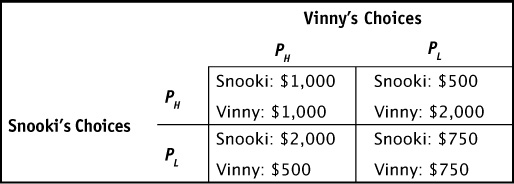
In a small town, there are two gas stations located on opposite sides of the highway. Snooki’s Stop and Go and Vinny’s Gas and Guzzle sell identical products, so consumers care only about who has the lowest price. Table 9-3 summarizes the daily revenue that each station would earn at each of two prices, one low (PL) and one high (PH). Naturally, Snooki’s revenue also depends upon Vinny’s pricing choice. We assume that they set the price in the morning simultaneously, and it cannot be changed.
TABLE 9-3 Game Matrix for Pricing Game

Let’s examine the situation. Once again we see dominant strategies in this game. No matter what price Vinny sets, Snooki’s revenues are higher if she sets the low price. No matter what price Snooki sets, Vinny’s revenues are higher if he also sets the low price. Setting the low price at the beginning of the day is a dominant strategy, and that is the Nash equilibrium.
Can they get out of this pricing dilemma? Not if the game is played only once. If the game is played repeatedly, like every day, Snooki and Vinny might learn to cooperate and set high prices every day. This cooperation, or tacit collusion, is believed to be common in oligopolies with a very small number of competing rivals. However, as in the prisoners’ dilemma, the temptation to “cheat” on the unspoken agreement by setting the low price one day is quite high. In repeated games, a firm that cheats one day can be punished the next day when the other firm also sets the low price. Such behavior is sometimes seen in industries like the airline industry when one company offers a discounted fare between two cities and rival airlines quickly counter with the same low fare.
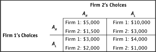
Both of the games previously discussed had two players with the same dominant strategy, and when dominant strategies converge, a Nash equilibrium outcome is clear to see. What happens if one or both firms do not have a dominant strategy? Table 9-4 shows the profits earned by two firms that can choose a high level of advertising (AH) spending or a low level (AL) of spending. Advertising is supposed to increase revenue, but it is also very costly and usually benefits larger firms with more customer loyalty. Firm 1 is a more established firm that will always earn more profit than Firm 2, so the payoffs are not symmetrical the way they were in the previous games.
TABLE 9-4 Game Matrix for Advertising Spending

Firm 1 has a clear choice: choose a high level of advertising spending. No matter what Firm 2 does, Firm 1’s profits are always higher when it chooses AH rather than AL. However, the decision isn’t so clear for Firm 2. The owner might have deliberations that go something like this:
• If Firm 1 is going to choose AL, I should choose AH because $2,000 is better than $1,000.
• But if Firm 1 is going to choose AH, I should choose AL because $3,000 is better than $1,500.
While it seems as if the owner of Firm 2 might flip-flop back and forth between her choices, because she can see that Firm 1 will always choose AH, Firm 2 will choose AL. Again this is a Nash equilibrium because, given the rival’s choice, neither firm would decide to change its choice away from the one that was made.
This chapter presented the imperfectly competitive market structures of monopolistic competition and oligopoly. Monopolistic competition shares characteristics of both perfect competition and monopoly. Because each firm has some product differentiation, the demand for the firm’s product is downward-sloping, and this gives the firm some degree of pricing power. It is possible for profits to be positive (or negative) in the short run, but in the long run, entry and exit of firms will bring profits back to zero. Oligopoly is a market structure that describes a broad group of real-world markets. The vast diversity of such markets makes it impossible to produce one general model that predicts how firms strategically behave when there is mutual interdependence. Game theory has been used to predict how a small number of rivals can either compete with each other or cooperate with each other. The simple prisoners’ dilemma and a related pricing game were presented to show how two rivals can pursue dominant strategies and how the outcome produces a Nash equilibrium.
Is each of the following statements true or false? Explain.
1. Like those in perfect competition, firms in monopolistic competition earn zero profit in the long run and, as with monopolies, deadweight loss is created.
2. The following is true of monopolistic competition in the long run:  .
.
3. Because of an absence of barriers to entry, firms in an oligopoly earn zero economic profit in the long run.
4. A Nash equilibrium is an outcome of a game such that each player earns the greatest payoff possible, no matter what the other player chooses.
For each of the following, choose the answer that best fits.
5. Which of the following is true of firms in monopolistic competition?
A. Product differentiation leads to a perfectly elastic demand curve for the firm’s product.
B. Barriers to entry ensure that long-run profits are positive.
C. Many firms exist, each with a small degree of price-setting ability.
D. Firms produce the allocatively and productively efficient level of output.
6. Doug’s Duds is a monopolistically competitive retail clothing store in Freshville. Doug is currently maximizing his profit, but that profit is negative. Given this, firms will _____ the Freshville retail clothing market, causing the demand for Doug’s Duds to _____, and causing prices to _____ until profits are _____.
A. exit; increase; increase; zero
B. exit; increase; decrease; zero
C. exit; decrease; increase; zero
D. enter; decrease; decrease; zero
7. Which of the following is true of firms in oligopoly?
A. In the long run, an absence of barriers to entry produces breakeven profits.
B. Firms are price takers.
C. The goods produced can be either identical or differentiated.
D. Firms act independently of one another.
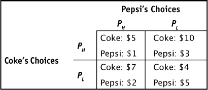
8. Suppose Coke and Pepsi are deciding whether to charge a high price or a low price for a case of soda. The game matrix in Table 9-6 shows the choices and payoffs for this game. If the game is played only once, are there any dominant strategies?

A. Yes. Choosing PH is the dominant strategy for both firms.
B. Yes. Choosing PL is the dominant strategy for Pepsi.
C. Yes. Choosing PL is the dominant strategy for both firms.
D. No. Neither firm has a dominant strategy.
9. Suppose Coke and Pepsi are deciding whether to charge a high price or a low price for a case of soda. The game matrix in Table 9-6 shows the choices and payoffs for this game. If the game is played only once, what is the outcome?
A. Both firms choose PH.
B. Both firms choose PL.
C. Coke chooses PH and Pepsi choose PL.
D. Pepsi chooses PH and Coke chooses PL.
10. Nike and Reebok are rival firms in the athletic shoe industry. When we say that they are mutually interdependent, this means that:
A. Nike’s actions affect Reebok, but Reebok’s actions do not affect Nike.
B. Nike’s actions do not affect Reebok, and Reebok’s actions do not affect Nike.
C. Reebok’s actions affect Nike, but Nike’s actions do not affect Reebok.
D. Nike’s actions affect Reebok, and Reebok’s actions affect Nike.