Chapter 12. Building a Knowledge Graph
In this book, we have been working through many blueprints for text analysis. Our goal was always to identify patterns in the data with the help of statistics and machine learning. In Chapter 10 we explained how embeddings can be used to answer questions like “What is to Germany like Paris is to France?” Embeddings represent some kind of implicit knowledge that was learned from the training documents based on a notion of similarity.
A knowledge base, in contrast, consists of structured statements of the form “Berlin capital-of Germany.” In this case, “capital-of” is a precisely defined relation between the two specific entities Berlin and Germany. The network formed by many entities and their relations is a graph in the mathematical sense, a knowledge graph. Figure 12-1 shows a simple knowledge graph illustrating the example. In this chapter, we will introduce blueprints to extract structured information from unstructured text and build a basic knowledge graph.

Figure 12-1. A simple knowledge graph.
What You’ll Learn and What We’ll Build
Information extraction is one of the hardest tasks in natural language processing because of the complexity and inherent ambiguity of language. Thus, we need to apply a sequence of different steps to discover the entities and relationships. Our example use case in this section is the creation of a knowledge graph based on business news articles about companies.
In the course of the chapter, we will take a deep dive into the advanced language processing features of spaCy. We will use the pretrained neural models in combination with custom rules for named-entity recognition, coreference resolution, and relation extraction. We will also explain the necessary steps to perform entity linking, but we won’t go into the implementation details.
After reading this chapter, you will have the basic linguistic and technical knowledge to start building your own knowledge base. You will find the source code for this chapter and additional information in our GitHub repository.
Knowledge Graphs
A knowledge graph is a large semantic network. It consists of nodes that are entities such as persons, places, events, or companies, and edges that represent formalized relations between those nodes, as shown in Figure 12-1.
All the big players such as Google, Microsoft, Facebook, etc., use knowledge graphs to power their search engines and query services.1 And nowadays more and more companies are building their own knowledge graphs to gain market insights or power chatbots. But the largest knowledge graph is distributed all over the world: Linked Open Data refers to all the available data on the web that can be identified by a uniform resource identifier (URI). It is the result of 20 years of academic development in the area of the Semantic Web (see “Semantic Web and RDF”).
The types of nodes and edges are precisely defined by an ontology, which is itself a knowledge base for the terminology used in a domain. For example, the public ontology Wikidata provides definitions for all types used in Figure 12-1.2 Each of these definitions has a unique URI (e.g., “city” is http://www.wikidata.org/wiki/Q515.). In fact, Wikidata contains both, the type definitions and the actual objects in a queryable format.
Information Extraction
There are several typical steps needed to extract structured information from text, as shown in Figure 12-2. As a first step, named-entity recognition, finds mentions of named entities in the text and labels them with the correct type, e.g., person, organization, or location. The same entity is usually referenced multiple times in a document by different variants of the name or by pronouns. The second step, coreference resolution, identifies and resolves those coreferences to prevent duplicates and information loss.
Closely related to coreference resolution, and usually the next step, is the task of entity linking. Here, the goal is to link a mention in the text to a unique real-world entity in an ontology, for example, Berlin to the URI http://www.wikidata.org/entity/Q64. Thus, any ambiguities are removed: Q64 is the Berlin in Germany and not the one in New Hampshire (which is, by the way, Q821244 in Wikidata). This is essential to connect information from different sources and really build a knowledge base.
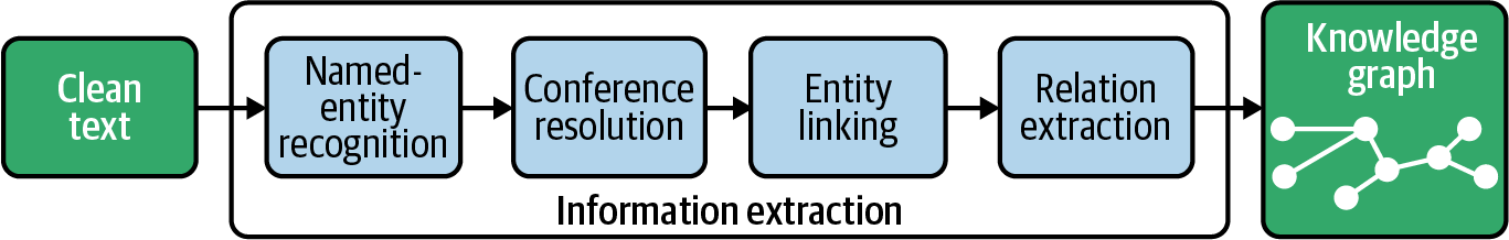
Figure 12-2. The process of information extraction.
The last step, relation extraction, identifies the relations between those entities. In an application scenario, you will usually consider only a few relations of interest because it is hard to extract this kind of information correctly from arbitrary text.
Finally, you could store the graph in a graph database as the backend of a knowledge-based application. Such graph databases store the data either as RDF triples (triple stores) or in the form of a property graph, where nodes and edges can have arbitrary attributes. Commonly used graph databases are, for example, GraphDB (triple store), Neo4j, and Grakn (property graphs).
For each of the steps, you have the choice between a rule-based approach and machine learning. We will use available models of spaCy and rules in addition. We will not train our own models, though. The usage of rules for the extraction of domain-specific knowledge has the advantage that you can get started quickly without training data. As we will see, the results allow some really interesting analyses. But if you plan to build a corporate knowledge base on a large scale, you may have to train your own models for named-entity and relationship detection as well as for entity linking.
Introducing the Dataset
Assume you are working in the financial business and want to track news on mergers and acquisitions. It would be great if you could automatically identify company names and the kind of deals they are involved in and make the results available in a knowledge base. In this chapter, we will explain the building blocks to extract some information about companies. For example, we will extract the relation “Company1 acquires Company2.”
To simulate such a scenario, we use a publicly available dataset, the well-known Reuters-21578 news corpus. It contains more than 20,000 news articles of 90 categories published by Reuters in 1987. This dataset was chosen because it is free and easy to get. In fact, it is available as one of the NLTK standard corpora, and you can simply download it with NLTK:
importnltknltk.download('reuters')
We will work only with articles from the acquisitions category (acq). To prepare it for our purposes, we loaded all articles into a single DataFrame and did some data cleaning following the blueprints in “Cleaning Text Data”. Clean data is crucial to recognize named-entities and relationships as the neural models benefit from well-structured sentences. For this dataset, we substituted HTML escapes, removed stock ticker symbols, replaced abbreviations like mln for million, and corrected some spelling mistakes. We also dropped the headlines because they are written in capital letters only. The complete article bodies are retained, though. All cleaning steps can be found in the notebook on GitHub. Let’s take a look at a sample of the cleaned articles in our DataFrame:
USAir Group Inc said a U.S. District Court in Pittsburgh issued a temporary
restraining order to prevent Trans World Airlines Inc from buying additional
USAir shares. USAir said the order was issued in response to its suit, charging
TWA chairman Carl Icahn and TWA violated federal laws and made misleading
statements. TWA last week said it owned 15 % of USAir's shares. It also offered
to buy the company for 52 dollars a share cash or 1.4 billion dollars.
So, this is the data we have in mind when we develop the blueprints for information extraction. However, most of the sentences in the following sections are simplified examples to better explain the concepts.
Named-Entity Recognition
After data cleaning, we can start with the first step of our information extraction process: named-entity recognition. Named-entity recognition was briefly introduced in Chapter 4 as part of spaCy’s standard pipeline. spaCy is our library of choice for all the blueprints in this chapter because it is fast and has an extensible API that we will utilize. But you could also use Stanza or Flair (see “Alternatives for NER: Stanza and Flair”).
spaCy provides trained NER models for many languages. The English models have been trained on the large OntoNotes5 corpus containing 18 different entity types. Table 12-1 lists a subset of these. The remaining types are for numeric entities.
| NER Type | Description | NER Type | Description |
|---|---|---|---|
| PERSON | People, including fictional | PRODUCT | Vehicles, weapons, foods, etc. (Not services) |
| NORP | Nationalities or religious or political groups | EVENT | Named hurricanes, battles, wars, sports events, etc. |
| FAC | Facilities: buildings, airports, highways, bridges, etc. | WORK_OF_ART | Titles of books, songs, etc. |
| ORG | Organizations: companies, agencies, institutions, etc. | LAW | Named documents made into laws |
| GPE | Countries, cities, states | LANGUAGE | Any named language |
| LOCATION | Non-GPE locations, mountain ranges, bodies of water |
The NER tagger is enabled by default when you load a language model. Let’s start by initializing an nlp object with the standard (small) English model en_core_web_sm and print the components of the NLP pipeline:4
nlp=spacy.load('en_core_web_sm')(*nlp.pipeline,sep='\n')
Out:
('tagger', <spacy.pipeline.pipes.Tagger object at 0x7f98ac6443a0>)
('parser', <spacy.pipeline.pipes.DependencyParser object at 0x7f98ac7a07c0>)
('ner', <spacy.pipeline.pipes.EntityRecognizer object at 0x7f98ac7a0760>)
Once the text is processed, we can access the named entities directly with doc.ents. Each entity has a text and a label describing the entity type. These attributes are used in the last line in the following code to print the list of entities recognized in this text:
text="""Hughes Tool Co Chairman W.A. Kistler said its merger withBaker International Corp was still under consideration.We hope to come soon to a mutual agreement, Kistler said.The directors of Baker filed a law suit in Texas to force Hughesto complete the merger."""doc=nlp(text)(*[(e.text,e.label_)foreindoc.ents],sep=' ')
Out:
(Hughes Tool Co, ORG) (W.A. Kistler, PERSON) (Baker International Corp, ORG)
(Kistler, ORG) (Baker, PERSON) (Texas, GPE) (Hughes, ORG)
With spaCy’s neat visualization module displacy, we can generate a visual representation of the sentence and its named entities. This is helpful to inspect the result:
fromspacyimportdisplacydisplacy.render(doc,style='ent')
Out:

In general, spaCy’s named-entity recognizer does a good job. In our example, it was able to detect all named entities. The labels of Kistler and Baker in the second and third sentence, however, are not correct. In fact, distinguishing between persons and organizations is quite a challenge for NER models because those entity types are used very similarly. We will resolve such problems later in the blueprint for name-based coreference resolution.
Blueprint: Using Rule-Based Named-Entity Recognition
If you want to identify domain-specific entities on which the model has not been trained, you can of course train your own model with spaCy. But training a model requires a lot of training data. Often it is sufficient to specify simple rules for custom entity types. In this section, we will show how to use rules to detect government organizations like the “Department of Justice” (or alternatively the “Justice Department”) in the Reuters dataset.
spaCy provides an EntityRuler for this purpose, a pipeline component that can be used in combination with or instead of the statistical named-entity recognizer. Compared to regular expression search, spaCy’s matching engine is more powerful because patterns are defined on sequences of spaCy’s tokens instead of just strings. Thus, you can use any token property like the lemma or the part-of-speech tag to build your patterns.
So, let’s define some pattern rules to match departments of the US government and the “Securities and Exchange Commission,” which is frequently mentioned in our corpus:
fromspacy.pipelineimportEntityRulerdepartments=['Justice','Transportation']patterns=[{"label":"GOV","pattern":[{"TEXT":"U.S.","OP":"?"},{"TEXT":"Department"},{"TEXT":"of"},{"TEXT":{"IN":departments},"ENT_TYPE":"ORG"}]},{"label":"GOV","pattern":[{"TEXT":"U.S.","OP":"?"},{"TEXT":{"IN":departments},"ENT_TYPE":"ORG"},{"TEXT":"Department"}]},{"label":"GOV","pattern":[{"TEXT":"Securities"},{"TEXT":"and"},{"TEXT":"Exchange"},{"TEXT":"Commission"}]}]
Each rule consists of a dictionary with a label, in our case the custom entity type GOV, and a pattern that the token sequence must match. You can specify multiple rules for the same label, as we did here.5 The first rule, for example, matches sequences of tokens with the texts "U.S." (optional, denoted by "OP": "?"), "Department", "of", and either "Justice" or "Transportation". Note that this and the second rule refine already recognized entities of type ORG. Thus, these patterns must be applied on top and not instead of spaCy’s named-entity model.
Based on these patterns, we create an EntityRuler and add it to our pipeline:
entity_ruler=EntityRuler(nlp,patterns=patterns,overwrite_ents=True)nlp.add_pipe(entity_ruler)
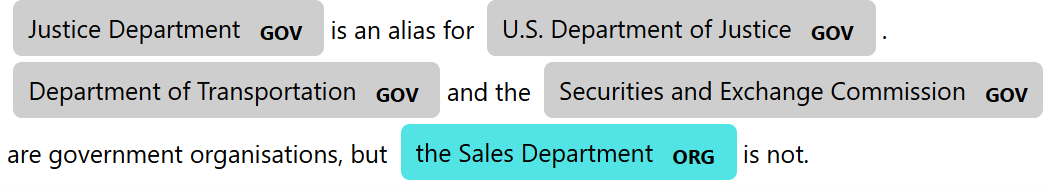
Now, when we call nlp, those organizations will automatically be labeled with the new type GOV:
text="""Justice Department is an alias for the U.S. Department of Justice.Department of Transportation and the Securities and Exchange Commissionare government organisations, but the Sales Department is not."""doc=nlp(text)displacy.render(doc,style='ent')
Out:
Blueprint: Normalizing Named Entities
One approach to simplify the resolution of different entity mentions to a single name is the normalization or standardization of mentions. Here, we will do a first normalization, which is generally helpful: the removal of unspecific suffixes and prefixes. Take a look at this example:
text="Baker International's shares climbed on the New York Stock Exchange."doc=nlp(text)(*[([t.textfortine],e.label_)foreindoc.ents],sep='\n')
Out:
(['Baker', 'International', "'s"], 'ORG')
(['the', 'New', 'York', 'Stock', 'Exchange'], 'ORG')
In the first sentence, the token sequence Baker International's was detected as an entity even though the genitive-s is not part of the company name. A similar case is the article in the New York Stock Exchange. Regardless of whether the article is actually part of the name or not, entities will likely be referenced sometimes with and sometimes without the article. Thus, the general removal of the article and an apostrophe-s simplifies the linking of mentions.
Warning
As with any rules, there is a potential of errors: think of The Wall Street Journal or McDonald's. If you need to preserve the article or the apostrophe-s in such cases, you must define exceptions for the rules.
Our blueprint function shows how to implement normalizations such as removing a leading article and a trailing apostrophe-s in spaCy. As we are not allowed to update entities in place, we create a copy of the entities and apply our modifications to this copy:
fromspacy.tokensimportSpandefnorm_entities(doc):ents=[]forentindoc.ents:ifent[0].pos_=="DET":# leading articleent=Span(doc,ent.start+1,ent.end,label=ent.label)ifent[-1].pos_=="PART":# trailing particle like 'sent=Span(doc,ent.start,ent.end-1,label=ent.label)ents.append(ent)doc.ents=tuple(ents)returndoc
An entity in spaCy is a Span object with a defined start and end plus an additional label denoting the type of the entity. We loop through the entities and adjust the position of the first and last token of the entity if necessary. Finally, we replace doc.ents with our modified copy.
The function takes a spaCy Doc object (named doc) as a parameter and returns a Doc. Therefore, we can use it as a another pipeline component and simply add it to the existing pipeline:
nlp.add_pipe(norm_entities)
Now we can repeat the process on the example sentences and check the result:
doc=nlp(text)(*[([t.textfortine],e.label_)foreindoc.ents],sep='\n')
Out:
(['Baker', 'International'], 'ORG')
(['New', 'York', 'Stock', 'Exchange'], 'ORG')
Merging Entity Tokens
In many cases, it makes sense to treat compound names like the ones from the previous example as single tokens because it simplifies the sentence structure. spaCy provides a built-in pipeline function merge_entities for that purpose. We add it to our NLP pipeline and get exactly one token per named-entity:
fromspacy.pipelineimportmerge_entitiesnlp.add_pipe(merge_entities)doc=nlp(text)(*[(t.text,t.ent_type_)fortindocift.ent_type_!=''])
Out:
('Baker International', 'ORG') ('New York Stock Exchange', 'ORG')
Even though merging entities simplifies our blueprints later in this chapter, it may not always be a good idea. Think, for example, about compound entity names like London Stock Exchange. After merging into a single token, the implicit relation of this entity to the city of London will be lost.
Coreference Resolution
One of the greatest obstacles in information extraction is the fact that entity mentions appear in many different spellings (also called surface forms). Look at the following sentences:
Hughes Tool Co Chairman W.A. Kistler said its merger with Baker International Corp. was still under consideration. We hope to come to a mutual agreement, Kistler said. Baker will force Hughes to complete the merger. A review by the U.S. Department of Justice was completed today. The Justice Department will block the merger after consultation with the SEC.
As we can see, entities are frequently introduced by their full name, while later mentions use abbreviated versions. This is one type of coreference that must resolved to understand what’s going on. Figure 12-3 shows a co-occurrence graph without (left) and with (right) unified names. Such a co-occurrence graph, as we will build in the next section, is a visualization of entity pairs appearing in the same article.

Figure 12-3. A co-occurrence graph of the same articles before (left) and after coreference resolution (right).
Coreference resolution is the task of determining the different mentions of an entity within a single text, for example, abbreviated names, aliases, or pronouns. The result of this step is a group of coreferencing mentions called a mention cluster, for example, {Hughes Tool Co, Hughes, its}. Our target in this section is to identify related mentions and link them within a document.
For this purpose, we develop a couple of blueprints for coreference resolution and name unification (see Figure 12-4). We will restrict ourselves to organizations and persons, as these are the entity types we are interested in. First, we will resolve aliases like SEC by a dictionary lookup. Then we will match names within a document to the first mention. For example, we will create a link from “Kistler” to “W.A. Kistler.” After that, indirect references (anaphora) like the pronoun its in the first sentence will be resolved. Finally, we will normalize again the names of the resolved entities. All of these steps will be implemented as additional pipeline functions.
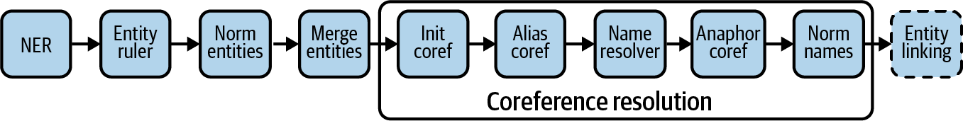
Figure 12-4. Pipeline for named-entity recognition and coreference resolution.
Entity linking goes one step further. Here the mentions of an entity are disambiguated on a semantic level and linked to a unique entry in an existing knowledge base. Because entity linking is itself a challenging task, we will not provide a blueprint for that but just discuss it at the end of this section.
Blueprint: Using spaCy’s Token Extensions
We need a way to technically create the link from the different mentions of an entity to the main reference, the referent. After coreference resolution, the token for “Kistler” of the example article should point to “(W.A. Kistler, PERSON).” spaCy’s extension mechanism allows us to define custom attributes, and this is the perfect way to store this kind of information with tokens. Thus, we create two token extensions ref_n (referent’s name) and ref_t (referent’s type). The attributes will be initialized for each token with the specified default values by spaCy for each token:
fromspacy.tokensimportTokenToken.set_extension('ref_n',default='')Token.set_extension('ref_t',default='')
The function init_coref shown next ensures that each entity mention of type ORG, GOV, and PERSON gets an initial reference to itself. This initialization is required for the succeeding functions:
definit_coref(doc):foreindoc.ents:ife.label_in['ORG','GOV','PERSON']:e[0]._.ref_n,e[0]._.ref_t=e.text,e.label_returndoc
The custom attributes are accessed via the underscore property of the token. Note that after merge_entities, each entity mention e consists of a single token e[0] where we set the attributes. We could also define the attributes on the entity spans instead of tokens, but we want to use the same mechanism for pronoun resolution later.
Blueprint: Performing Alias Resolution
Our first targets are well-known domain aliases like Transportation Department for “U.S. Department of Transportation” and acronyms like SEC or TWA. A simple solution to resolve such aliases is to use a lookup dictionary. We prepared such a dictionary for all the acronyms and some common aliases of the Reuters corpus and provided it as part of the blueprints module for this chapter.6 Here are some example lookups:
fromblueprints.knowledgeimportalias_lookupfortokenin['Transportation Department','DOT','SEC','TWA']:(token,':',alias_lookup[token])
Out:
Transportation Department : ('U.S. Department of Transportation', 'GOV')
DOT : ('U.S. Department of Transportation', 'GOV')
SEC : ('Securities and Exchange Commission', 'GOV')
TWA : ('Trans World Airlines Inc', 'ORG')
Each token alias is mapped to a tuple consisting of an entity name and a type. The function alias_resolver shown next checks whether an entity’s text is found in the dictionary. If so, its ref attributes are updated to the looked-up value:
defalias_resolver(doc):"""Lookup aliases and store result in ref_t, ref_n"""forentindoc.ents:token=ent[0].textiftokeninalias_lookup:a_name,a_type=alias_lookup[token]ent[0]._.ref_n,ent[0]._.ref_t=a_name,a_typereturnpropagate_ent_type(doc)
Once we have resolved the aliases, we can also correct the type of the named-entity in case it was misidentified. This is done by the function propagate_ent_type. It updates all resolved aliases and will also be used in the next blueprint for name-based coreference resolution:
defpropagate_ent_type(doc):"""propagate entity type stored in ref_t"""ents=[]foreindoc.ents:ife[0]._.ref_n!='':# if e is a coreferencee=Span(doc,e.start,e.end,label=e[0]._.ref_t)ents.append(e)doc.ents=tuple(ents)returndoc
Again, we add the alias_resolver to our pipeline:
nlp.add_pipe(alias_resolver)
Now we can inspect the results. For this purpose, our provided blueprints package includes a utility function display_ner that creates a DataFrame for the tokens in a doc object with the relevant attributes for this chapter:
fromblueprints.knowledgeimportdisplay_nertext="""The deal of Trans World Airlines is under investigation by theU.S. Department of Transportation.The Transportation Department will block the deal of TWA."""doc=nlp(text)display_ner(doc).query("ref_n != ''")[['text','ent_type','ref_n','ref_t']]
Out:
| text | ent_type | ref_n | ref_t | |
|---|---|---|---|---|
| 3 | Trans World Airlines | ORG | Trans World Airlines Inc | ORG |
| 9 | U.S. Department of Transportation | GOV | U.S. Department of Transportation | GOV |
| 12 | Transportation Department | GOV | U.S. Department of Transportation | GOV |
| 18 | TWA | ORG | Trans World Airlines Inc | ORG |
Blueprint: Resolving Name Variations
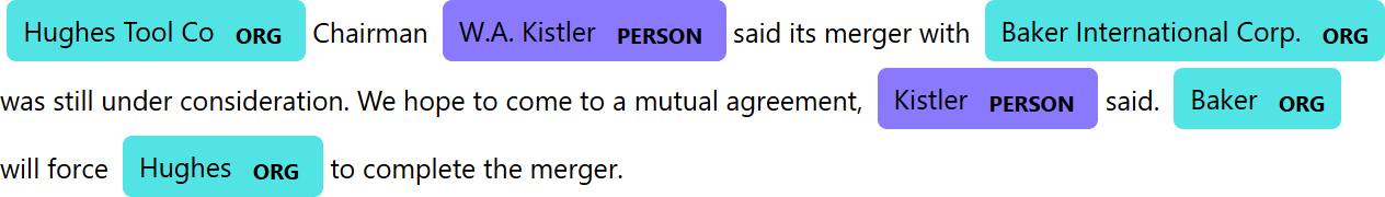
Alias resolution works only if the aliases are known up front. But because articles contain variations of almost any names, it is not feasible to build a dictionary for all of them. Take a look again at the recognized named entities in the first sentences of our introductory example:

Here you find the coreference “Kistler” for W.A. Kistler (PERSON), “Baker” for Baker International Corp (ORG), and “Hughes” for Hughes Tool Co (ORG). And as you can see, abbreviated company names are often mistaken for people, especially when they are used in impersonated form, as in the examples. In this blueprint, we will resolve those coreferences and assign the correct entity types to each mention.
For that, we will exploit a common pattern in news articles. An entity is usually introduced first by its full name, while later mentions use abbreviated versions. Thus, we will resolve the secondary references by matching the names to the first mention of an entity. Of course, this is a heuristic rule that could produce false matches. For example, Hughes could also refer in the same article to the company and to the legendary entrepreneur Howard Hughes (who indeed founded Hughes Tool Co.). But such cases are rare in our dataset, and we decide to accept that uncertainty in favor of the many cases where our heuristics works correctly.
We define a simple rule for name matching: a secondary mention matches a primary mention if all of its words appear in the primary mention in the same order. To check this, the function name_match shown next transforms a secondary mention m2 into a regular expression and searches for a match in the primary mention m1:
defname_match(m1,m2):m2=re.sub(r'[()\.]','',m2)# ignore parentheses and dotsm2=r'\b'+m2+r'\b'# \b marks word boundarym2=re.sub(r'\s+',r'\\b.*\\b',m2)returnre.search(m2,m1,flags=re.I)isnotNone
The secondary mention of Hughes Co., for example, would be converted into '\bHughes\b.*\bCo\b', which matches Hughes Tool Co. The \b ensures that only whole words match and not subwords like Hugh.
Based on this matching logic, the function name_resolver shown next implements the name-based coreference resolution for organizations and persons:
defname_resolver(doc):"""create name-based reference to e1 as primary mention of e2"""ents=[eforeindoc.entsife.label_in['ORG','PERSON']]fori,e1inenumerate(ents):fore2inents[i+1:]:ifname_match(e1[0]._.ref_n,e2[0].text):e2[0]._.ref_n=e1[0]._.ref_ne2[0]._.ref_t=e1[0]._.ref_treturnpropagate_ent_type(doc)
First, we create a list of all organization and person entities. Then all pairs of entities e1 and e2 are compared against each other. The logic ensures that entity e1 always comes before e2 in the document. If e2 matches e1, its referent is set to the same as in e1. Thus, the first matching entity is automatically propagated to its subsequent coreferences.
We add this function to the nlp pipeline and check the result:
nlp.add_pipe(name_resolver)doc=nlp(text)displacy.render(doc,style='ent')
Out:
Now each named-entity in our example has the correct type. We can also check that the entities are mapped to their first mention:
display_ner(doc).query("ref_n != ''")[['text','ent_type','ref_n','ref_t']]
Out:
| text | ent_type | ref_n | ref_t | |
|---|---|---|---|---|
| 0 | Hughes Tool Co | ORG | Hughes Tool Co | ORG |
| 2 | W.A. Kistler | PERSON | W.A. Kistler | PERSON |
| 7 | Baker International Corp. | ORG | Baker International Corp. | ORG |
| 22 | Kistler | PERSON | W.A. Kistler | PERSON |
| 25 | Baker | ORG | Baker International Corp. | ORG |
| 28 | Hughes | ORG | Hughes Tool Co | ORG |
Blueprint: Performing Anaphora Resolution with NeuralCoref
In linguistics, anaphora are words whose interpretation depends on the preceding text. Consider this variation of our example sentences:
text="""Hughes Tool Co said its merger with Bakerwas still under consideration. Hughes had a board meeting today.W.A. Kistler mentioned that the company hopes for a mutual agreement.He is reasonably confident."""
Here its, the company, and he are anaphora. NeuralCoref from Hugging Face is a library to resolve these kind of coreferences. The algorithm uses feature vectors based on word embeddings (see Chapter 10) in combination with two neural networks to identify coreference clusters and their main mentions.7
NeuralCoref is implemented as a pipeline extension for spaCy, so it fits perfectly into our process. We create the neural coreference resolver with a greedyness value of 0.45 and add it to our pipeline. The greedyness controls the sensitivity of the model, and after some experiments, we decided to choose a little more restrictive (better accuracy, lower recall) value than the default 0.5:
fromneuralcorefimportNeuralCorefneural_coref=NeuralCoref(nlp.vocab,greedyness=0.45)nlp.add_pipe(neural_coref,name='neural_coref')
NeuralCoref uses also spaCy’s extension mechanism to add custom attributes to Doc, Span, and Token objects. When a text is processed, we can access the detected coreference clusters with the doc._.coref_clusters attribute. In our example, three such clusters have been identified:
doc=nlp(text)(*doc._.coref_clusters,sep='\n')
Out:
Hughes Tool Co: [Hughes Tool Co, its]
Hughes: [Hughes, the company]
W.A. Kistler: [W.A. Kistler, He]
NeuralCoref works on Span objects (sequences of token) because coreferences in general are not limited to named entities. Thus, the blueprint function anaphor_coref retrieves for each token the first coreference cluster and searches for the first named-entity with a value in its ref_n attribute. In our case, this will be organizations and people only. Once found, it sets the values in ref_n and ref_t of the anaphor token to the same values as in the primary reference:
defanaphor_coref(doc):"""anaphora resolution"""fortokenindoc:# if token is coref and not already dereferencediftoken._.in_corefandtoken._.ref_n=='':ref_span=token._.coref_clusters[0].main# get referred spaniflen(ref_span)<=3:# consider only short spansforrefinref_span:# find first dereferenced entityifref._.ref_n!='':token._.ref_n=ref._.ref_ntoken._.ref_t=ref._.ref_tbreakreturndoc
Again, we add this resolver to our pipeline and check the result:
nlp.add_pipe(anaphor_coref)doc=nlp(text)display_ner(doc).query("ref_n != ''")\[['text','ent_type','main_coref','ref_n','ref_t']]
Out:
| text | ent_type | main_coref | ref_n | ref_t | |
|---|---|---|---|---|---|
| 0 | Hughes Tool Co | ORG | Hughes Tool Co | Hughes Tool Co | ORG |
| 2 | its | Hughes Tool Co | Hughes Tool Co | ORG | |
| 5 | Baker | PERSON | None | Baker | PERSON |
| 11 | Hughes | ORG | Hughes | Hughes Tool Co | ORG |
| 18 | W.A. Kistler | PERSON | W.A. Kistler | W.A. Kistler | PERSON |
| 21 | the | Hughes | Hughes Tool Co | ORG | |
| 22 | company | Hughes | Hughes Tool Co | ORG | |
| 29 | He | W.A. Kistler | W.A. Kistler | PERSON |
Now our pipeline consists of all the steps shown in Figure 12-4.
Name Normalization
Even though our name resolution unifies company mentions within an article, the company names are still inconsistent across articles. We find Hughes Tool Co. in one article and Hughes Tool in another one. An entity linker can be used to link different entity mentions to a unique canonical representation, but in absence of an entity linker we will use the (resolved) name entity as its unique identifier. Because of the previous steps for coreference resolution, the resolved names are always the first, and thus usually most complete, mentions in an article. So, the potential for errors is not that large.
Still, we have to harmonize company mentions by removing the legal suffixes like Co. or Inc. from company names. The following function uses a regular expression to achieve this:
defstrip_legal_suffix(text):returnre.sub(r'(\s+and)?(\s+|\b(Co|Corp|Inc|Plc|Ltd)\b\.?)*$','',text)(strip_legal_suffix('Hughes Tool Co'))
Out:
Hughes Tool
The last pipeline function norm_names applies this final normalization to each of the coreference-resolved organization names stored in the ref_n attributes. Note that Hughes (PERSON) and Hughes (ORG) will still remain separate entities with this approach.
defnorm_names(doc):fortindoc:ift._.ref_n!=''andt._.ref_tin['ORG']:t._.ref_n=strip_legal_suffix(t._.ref_n)ift._.ref_n=='':t._.ref_t=''returndocnlp.add_pipe(norm_names)
Sometimes the named-entity recognizer misclassifies a legal suffix like Co. or Inc. by itself as named-entity. If such an entity name gets stripped to the empty string, we just ignore it for later processing.
Entity Linking
In the previous sections we developed a pipeline of operations with the purpose of unifying the different mentions of named entities. But all this is string based, and except for the syntactical representation, we have no connection between the string U.S. Department of Justice and the represented real-world entity. The task of an entity linker, in contrast, is to resolve named entities globally and link them to a uniquely identified real-world entity. Entity linking makes the step from “strings to things.”8
Technically, this means that each mention is mapped to a URI. URIs, in turn, address entities in an existing knowledge base. This can be a public ontology, like Wikidata or DBpedia, or a private knowledge base in your company. URIs can be URLs (e.g., web pages) but do not have to be. The U.S. Department of Justice, for example, has the Wikidata URI http://www.wikidata.org/entity/Q1553390, which is also a web page where you find information about this entity. If you build your own knowledge base, it is not necessary to have a web page for each URI; they just must be unique. DBpedia and Wikidata, by the way, use different URIs, but you will find the Wikidata URI on DBpedia as a cross-reference. Both, of course, contain links to the Wikipedia web page.
Entity linking is simple if an entity is mentioned by a fully qualified name, like the U.S. Department of Justice. But the term Department of Justice without U.S. is already quite ambiguous because many states have a “Department of Justice.” The actual meaning depends on the context, and the task of an entity linker is to map such an ambiguous mention context-sensitively to the correct URI. This is quite a challenge and still an area of ongoing research. A common solution for entity linking in business projects is the usage of a public service (see “Services for Entity Linking”).
Alternatively, you could create your own entity linker. A simple solution would be a name-based lookup dictionary. But that does not take the context into account and would not resolve ambiguous names for different entities. For that, you need a more sophisticated approach. State-of-the-art solutions use embeddings and neural models for entity linking. spaCy also provides such an entity linking functionality. To use spaCy’s entity linker, you first have to create embeddings (see Chapter 10) for the real-world entities, which capture their semantics based on descriptions you specify. Then you can train a model to learn the context-sensitive mapping of mentions to the correct URI. The setup and training of an entity linker are, however, beyond the scope of this chapter.
Blueprint: Creating a Co-Occurrence Graph
In the previous sections, we spent much effort to normalize named entities and to resolve at least the in-document coreferences. Now we are finally ready to analyze a first relationship among pairs of entities: their joint mention in an article. For this, we will create a co-occurrence graph, the simplest form of a knowledge graph. The nodes in the co-occurrence graph are the entities, e.g., organizations. Two entities share an (undirected) edge if they are mentioned in the same context, for example, within an article, a paragraph, or a sentence.
Figure 12-5 shows part of the co-occurrence graph for companies mentioned together in articles of the Reuters corpus. The width of the edges visualizes the co-occurrence frequency. The modularity, a structural measure to identify closely related groups or communities in a network, was used to colorize the nodes and edges.9

Figure 12-5. Largest connected component of the co-occurrence graph generated from the Reuters corpus.
Of course, we don’t know anything about the type of relationship here. In fact, the joint mentioning of two entities merely indicates that there might be some relationship. We won’t know for sure unless we really analyze the sentences, and we will do that in the next section. But even the simple exploration of co-occurrences can already be revealing. For example, the central node in Figure 12-5 is the “Securities and Exchange Commission” because it is mentioned in many articles together with a great variety of other entities. Obviously, this entity plays a major role in mergers and acquisitions. The different clusters give us an impression about groups of companies (or communities) involved in certain deals.
To plot a co-occurrence graph, we have to extract entity pairs from a document. For longer articles covering multiple topic areas, it may be better to search for co-occurrences within paragraphs or even sentences. But the Reuters articles on mergers and acquisitions are very focused, so we stick to the document level here. Let’s briefly walk through the process to extract and visualize co-occurrences.
Extracting Co-Occurrences from a Document
The function extract_coocs returns the list of entities pairs of the specified types from a given Doc object:
fromitertoolsimportcombinationsdefextract_coocs(doc,include_types):ents=set([(e[0]._.ref_n,e[0]._.ref_t)foreindoc.entsife[0]._.ref_tininclude_types])yield fromcombinations(sorted(ents),2)
We first create a set of the coreference-resolved entity names and types. Having this, we use the function combinations from the Python standard library itertools to create all the entity pairs. Each pair is sorted lexicographically (sorted(ents)) to prevent duplicate entries like “(Baker, Hughes)” and “(Hughes, Baker).”
To process the whole dataset efficiently, we use again spaCy’s streaming by calling nlp.pipe (introduced in Chapter 4). As we do not need anaphora resolution to find in-document co-occurrences, we disable the respective components here:
batch_size=100coocs=[]foriinrange(0,len(df),batch_size):docs=nlp.pipe(df['text'][i:i+batch_size],disable=['neural_coref','anaphor_coref'])forj,docinenumerate(docs):coocs.extend([(df.index[i+j],*c)forcinextract_coocs(doc,['ORG','GOV'])])
Let’s take a look at the identified co-occurrences of the first article:
(*coocs[:3],sep='\n')
Out:
(10, ('Computer Terminal Systems', 'ORG'), ('Sedio N.V.', 'ORG'))
(10, ('Computer Terminal Systems', 'ORG'), ('Woodco', 'ORG'))
(10, ('Sedio N.V.', 'ORG'), ('Woodco', 'ORG'))
In information extraction, it is always recommended to have some kind of traceability that allows you to identify the source of the information in the case of problems. Therefore, we retain the index of the article, which in our case is the file ID of the Reuters corpus, with each co-occurrence tuple (here the ID 10). Based on this list, we generate a DataFrame with exactly one entry per entity combination, its frequency, and the article IDs (limited to five) where this co-occurrence was found.
coocs=[([id],*e1,*e2)for(id,e1,e2)incoocs]cooc_df=pd.DataFrame.from_records(coocs,columns=('article_id','ent1','type1','ent2','type2'))cooc_df=cooc_df.groupby(['ent1','type1','ent2','type2'])['article_id']\.agg(['count','sum'])\.rename(columns={'count':'freq','sum':'articles'})\.reset_index().sort_values('freq',ascending=False)cooc_df['articles']=cooc_df['articles'].map(lambdalst:','.join([str(a)forainlst[:5]]))
Here are the three most frequent entity pairs we found in the corpus:
cooc_df.head(3)
Out:
| ent1 | type1 | ent2 | type2 | freq | articles | |
|---|---|---|---|---|---|---|
| 12667 | Trans World Airlines | ORG | USAir Group | ORG | 22 | 1735,1771,1836,1862,1996 |
| 5321 | Cyclops | ORG | Dixons Group | ORG | 21 | 4303,4933,6093,6402,7110 |
| 12731 | U.S. Department of Transportation | GOV | USAir Group | ORG | 20 | 1735,1996,2128,2546,2799 |
Visualizing the Graph with Gephi
Actually, this DataFrame already represents the list of edges for our graph. For the visualization we prefer Gephi, an open source tool for graph analysis. Because it is interactive, it is much better to use than Python’s graph library NetworkX.10 To work with Gephi, we need to save the list of nodes and edges of the graph in Graph Exchange XML format. Fortunately, NetworkX provides a function to export graphs in this format. So, we can simply convert our DataFrame into a NetworkX graph and save it as a .gexf file. We discard rare entity pairs to keep the graph compact and rename the frequency column because Gephi automatically uses a weight attribute to adjust the width of edges:
importnetworkxasnxgraph=nx.from_pandas_edgelist(cooc_df[['ent1','ent2','articles','freq']]\.query('freq > 3').rename(columns={'freq':'weight'}),source='ent1',target='ent2',edge_attr=True)nx.readwrite.write_gexf(graph,'cooc.gexf',encoding='utf-8',prettyprint=True,version='1.2draft')
After importing the file into Gephi, we selected only the largest component (connected subgraph) and removed some nodes with only a few connections manually for the sake of clarity.11 The result is presented in Figure 12-5.
Note
Sometimes the most interesting relations are the ones that are not frequent. Take, for example, the first announcement on an upcoming merger or surprising relations that were mentioned a few times in the past but then forgotten. A sudden co-occurrence of entities that were previously unrelated can be a signal to start a deeper analysis of the relation.
Relation Extraction
Even though the co-occurrence graph already gave us some interesting insights about company networks, it does not tell us anything about the types of the relations. Take, for example, the subgraph formed by the companies Schlumberger, Fairchild Semiconductor, and Fujitsu in the lower-left corner of Figure 12-5. So far, we know nothing about the relations between those companies; the information is still hidden in sentences like these:
Fujitsu wants to expand. It plans to acquire 80% of Fairchild Corp, an industrial unit of Schlumberger.
In this section, we will introduce two blueprints for pattern-based relation extraction. The first and simpler blueprint searches for token phrases of the form “subject-predicate-object.” The second one uses the syntactical structure of a sentence, the dependency tree, to get more precise results at the price of more complex rules. In the end, we will generate a knowledge graph based on the four relations: acquires, sells, subsidiary-of, and chairperson-of. To be honest, we will use relaxed definitions of acquires and sells, which are easier to identify. They will also match sentences like “Fujitsu plans to acquire 80% of Fairchild Corp” or even “Fujitsu withdraws the option to acquire Fairchild Corp.”
Relation extraction is a complicated problem because of the ambiguity of natural language and the many different kinds and variations of relations. Model-based approaches to relation extraction are a current topic in research.12 There are also some training datasets like FewRel publicly available. However, training a model to identify relations is still pretty much in the research stage and out of the scope of this book.
Blueprint: Extracting Relations Using Phrase Matching
The first blueprint works like rule-based entity recognition: it tries to identify relations based on patterns for token sequences. Let’s start with a simplified version of the introductory example to explain the approach.
text="""Fujitsu plans to acquire 80% of Fairchild Corp, an industrial unitof Schlumberger."""
We could find the relations in this sentence by searching for patterns like these:
ORG {optional words, not ORG} acquire {optional words, not ORG} ORG
ORG {optional words, not ORG} unit of {optional words, not ORG} ORG
spaCy’s rule-based matcher allows us to find patterns that not only can involve the textual tokens but also their properties, like the lemma or part of speech. To use it, we must first define a matcher object. Then we can add rules with token patternsto the matcher:
fromspacy.matcherimportMatchermatcher=Matcher(nlp.vocab)acq_synonyms=['acquire','buy','purchase']pattern=[{'_':{'ref_t':'ORG'}},# subject{'_':{'ref_t':{'NOT_IN':['ORG']}},'OP':'*'},{'POS':'VERB','LEMMA':{'IN':acq_synonyms}},{'_':{'ref_t':{'NOT_IN':['ORG']}},'OP':'*'},{'_':{'ref_t':'ORG'}}]# objectmatcher.add('acquires',None,pattern)
subs_synonyms=['subsidiary','unit']pattern=[{'_':{'ref_t':'ORG'}},# subject{'_':{'ref_t':{'NOT_IN':['ORG']}},'POS':{'NOT_IN':['VERB']},'OP':'*'},{'LOWER':{'IN':subs_synonyms}},{'TEXT':'of'},{'_':{'ref_t':{'NOT_IN':['ORG']}},'POS':{'NOT_IN':['VERB']},'OP':'*'},{'_':{'ref_t':'ORG'}}]# objectmatcher.add('subsidiary-of',None,pattern)
The first pattern is for the acquires relation. It returns all spans consisting of an organization, followed by arbitrary tokens that are not organizations, a verb matching several synonyms of acquire, again arbitrary tokens, and finally the second organization. The second pattern for subsidiary-of works similarly.
Granted, the expressions are hard to read. One reason is that we used the custom attribute ref_t instead of the standard ENT_TYPE. This is necessary to match coreferences that are not marked as entities, e.g., pronouns. Another one is that we have included some NOT_IN clauses. This is because rules with the asterisk operator (*) are always dangerous as they search patterns of unbounded length. Additional conditions on the tokens can reduce the risk for false matches. For example, we want to match “Fairchild, an industrial unit of Schlumberger” for the subsidiary-of relation, but not “Fujitsu mentioned a unit of Schlumberger.” When developing rules, you always have to pay for precision with complexity. We will discuss the problems of the acquires relation on that aspect in a minute.
The blueprint function extract_rel_match now takes a processed Doc object and a matcher and transforms all matches to subject-predicate-object triples:
defextract_rel_match(doc,matcher):forsentindoc.sents:formatch_id,start,endinmatcher(sent):span=sent[start:end]# matched spanpred=nlp.vocab.strings[match_id]# rule namesubj,obj=span[0],span[-1]ifpred.startswith('rev-'):# reversed relationsubj,obj=obj,subjpred=pred[4:]yield((subj._.ref_n,subj._.ref_t),pred,(obj._.ref_n,obj._.ref_t))
The predicate is determined by the name of the rule; the involved entities are simply the first and last tokens of the matched span. We restrict the search to the sentence level because in a whole document we would have a high risk of finding false positives spanning multiple sentences.
Usually, the rules match in the order “subject-predicate-object,” but often the entities appear in the text in reversed order, like in “the Schlumberger unit Fairchild Corp.” Here, the order of entities with regard to the subsidiary-of relation is “object-predicate-subject.” extract_rel_match is prepared to handle this and switches the subject and object if a rule has the prefix rev- like this one:
pattern=[{'_':{'ref_t':'ORG'}},# subject{'LOWER':{'IN':subs_synonyms}},# predicate{'_':{'ref_t':'ORG'}}]# objectmatcher.add('rev-subsidiary-of',None,pattern)
Now we are able to detect acquires and both variants of subsidiary-of in sentences like these:
text="""Fujitsu plans to acquire 80% of Fairchild Corp, an industrial unitof Schlumberger. The Schlumberger unit Fairchild Corp received an offer."""doc=nlp(text)(*extract_rel_match(doc,matcher),sep='\n')
Out:
(('Fujitsu', 'ORG'), 'acquires', ('Fairchild', 'ORG'))
(('Fairchild', 'ORG'), 'subsidiary-of', ('Schlumberger', 'ORG'))
(('Fairchild', 'ORG'), 'subsidiary-of', ('Schlumberger', 'ORG'))
Although the rules work nicely for our examples, the rule for acquires is not very reliable. The verb acquire can appear in many different constellations of entities. Thus, there is a high probability for false matches like this one:
text="Fairchild Corp was acquired by Fujitsu."(*extract_rel_match(nlp(text),matcher),sep='\n')
Out:
(('Fairchild', 'ORG'), 'acquires', ('Fujitsu', 'ORG'))
Or this one:
text="Fujitsu, a competitor of NEC, acquired Fairchild Corp."(*extract_rel_match(nlp(text),matcher),sep='\n')
Out:
(('NEC', 'ORG'), 'acquires', ('Fairchild', 'ORG'))
Obviously, our rule wasn’t made for passive clauses (“was acquired by”) where the subject and object switch positions. We also cannot handle insertions containing named entities or negations because they produce false matches. To treat those cases correctly, we need knowledge about the syntactical structure of the sentence. And we get that from the dependency tree.
But let’s first remove the unreliable rule for acquires from the matcher:
ifmatcher.has_key("acquires"):matcher.remove("acquires")
Blueprint: Extracting Relations Using Dependency Trees
The grammatical rules of a language impose a syntactical structure on each sentence. Each word serves a certain role in relation to the other words. A noun, for example, can be the subject or the object in a sentence; it depends on its relation to the verb. In linguistic theory, the words of a sentence are hierarchically interdependent, and the task of the parser in an NLP pipeline is to reconstruct these dependencies.13 The result is a dependency tree, which can also be visualized by displacy:
text="Fujitsu, a competitor of NEC, acquired Fairchild Corp."doc=nlp(text)displacy.render(doc,style='dep',options={'compact':False,'distance':100})
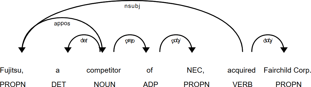
Each node in the dependency tree represents a word. The edges are labeled with the dependency information. The root is usually the predicate of the sentence, in this case acquired, having a subject (nsubj) and an object (obj) as direct children. This first level, root plus children, already represents the essence of the sentence “Fujitsu acquired Fairchild Corp.”
Let’s also take a look at the example with the passive clause. In this case, the auxiliary verb (auxpass) signals that acquired was used in passive form and Fairchild is the passive subject (nsubjpass):

Warning
The values of the dependency labels depend on the corpus the parser model was trained on. They are also language dependent because different languages have different grammar rules. So, you definitely need to check which tag set is used by the dependency parser.
The function extract_rel_dep implements a rule to identify verb-based relations like acquires based on the dependencies:
defextract_rel_dep(doc,pred_name,pred_synonyms,excl_prepos=[]):fortokenindoc:iftoken.pos_=='VERB'andtoken.lemma_inpred_synonyms:pred=tokenpassive=is_passive(pred)subj=find_subj(pred,'ORG',passive)ifsubjisnotNone:obj=find_obj(pred,'ORG',excl_prepos)ifobjisnotNone:ifpassive:# switch rolesobj,subj=subj,objyield((subj._.ref_n,subj._.ref_t),pred_name,(obj._.ref_n,obj._.ref_t))
The main loop iterates through all tokens in a doc and searches for a verb signaling our relationship. This condition is the same as in the flat pattern rule we used before. But when we detect a possible predicate, we now traverse the dependency tree to find the correct subject and the object. find_subj searches the left subtree, and find_obj searches the right subtree of the predicate. Those functions are not printed in the book, but you can find them in the GitHub notebook for this chapter. They use breadth-first search to find the closest subject and object, as nested sentences may have multiple subjects and objects. Finally, if the predicate indicates a passive clause, the subject and object will be swapped.
Note, that this function also works for the sells relation:
text="""Fujitsu said that Schlumberger Ltd has arrangedto sell its stake in Fairchild Inc."""doc=nlp(text)(*extract_rel_dep(doc,'sells',['sell']),sep='\n')
Out:
(('Schlumberger', 'ORG'), 'sells', ('Fairchild', 'ORG'))
In this case, Fairchild Inc. is the closest object in the dependency tree to sell and identified correctly as the object of the investigated relation. But to be the “closest” is not always sufficient. Consider this example:
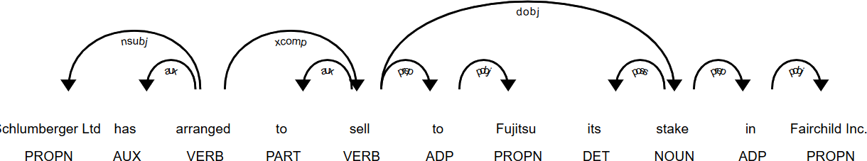
Actually, we have a three-way relation here: Schlumberger sells Fairchild to Fujitsu. Our sells relation is intended to have the meaning “one company sells [whole or parts of] another company.” The other part is covered by the acquires relation. But how can we detect the right object here? Both Fujitsu and Fairchild are prepositional objects in this sentence (dependency pobj), and Fujitsu is the closest. The preposition is the key: Schlumberger sells something “to” Fujitsu, so that’s not the relation we are looking for. The purpose of the parameter excl_prepos in the extraction function is to skip objects with the specified prepositions. Here is the output without (A) and with (B) preposition filter:
("A:",*extract_rel_dep(doc,'sells',['sell']))("B:",*extract_rel_dep(doc,'sells',['sell'],['to','from']))
Out:
A: (('Schlumberger', 'ORG'), 'sells', ('Fujitsu', 'ORG'))
B:
Let’s check how our new relation extraction function works on a few variations of the examples:
texts=["Fairchild Corp was bought by Fujitsu.",# 1"Fujitsu, a competitor of NEC Co, acquired Fairchild Inc.",# 2"Fujitsu is expanding."+"The company made an offer to acquire 80% of Fairchild Inc.",# 3"Fujitsu plans to acquire 80% of Fairchild Corp.",# 4"Fujitsu plans not to acquire Fairchild Corp.",# 5"The competition forced Fujitsu to acquire Fairchild Corp."# 6]acq_synonyms=['acquire','buy','purchase']fori,textinenumerate(texts):doc=nlp(text)rels=extract_rel_dep(doc,'acquires',acq_synonyms,['to','from'])(f'{i+1}:',*rels)
Out:
1: (('Fujitsu', 'ORG'), 'acquires', ('Fairchild', 'ORG'))
2: (('Fujitsu', 'ORG'), 'acquires', ('Fairchild', 'ORG'))
3: (('Fujitsu', 'ORG'), 'acquires', ('Fairchild', 'ORG'))
4: (('Fujitsu', 'ORG'), 'acquires', ('Fairchild', 'ORG'))
5: (('Fujitsu', 'ORG'), 'acquires', ('Fairchild', 'ORG'))
6:
As we can see, the relations in the first four sentences have been correctly extracted. Sentence 5, however, contains a negation and still returns acquires. This is a typical case of a false positive. We could extend our rules to handle this case correctly, but negations are rare in our corpus, and we accept the uncertainty in favor of the simpler algorithm. Sentence 6, in contrast, is an example for a possible false negative. Even though the relation was mentioned, it was not detected because the subject in this sentence is competition and not one of the companies.
Actually, dependency-based rules are inherently complex, and every approach to make them more precise results in even more complexity. It is a challenge to find a good balance between precision (fewer false positives) and recall (fewer false negatives) without making the code too complex.
Despite those deficiencies, the dependency-based rule still yields good results. This last step in the process, however, depends on the correctness of named-entity recognition, coreference resolution, and dependency parsing, all of which are not working with 100% accuracy. So, there will always be some false positives and false negatives. But the approach is good enough to produce highly interesting knowledge graphs, as we will do in the next section.
Creating the Knowledge Graph
Now that we know how to extract certain relationships, we can put everything together and create a knowledge graph from the entire Reuters corpus. We will extract organizations, persons and the four relations “acquires,” “sells,” “subsidiary-of,” and “executive-of.” Figure 12-6 shows the resulting graph with some selected subgraphs.
To get the best results in dependency parsing and named-entity recognition, we use spaCy’s large model with our complete pipeline. If possible, we will use the GPU to speed up NLP processing:
ifspacy.prefer_gpu():("Working on GPU.")else:("No GPU found, working on CPU.")nlp=spacy.load('en_core_web_lg')
pipes=[entity_ruler,norm_entities,merge_entities,init_coref,alias_resolver,name_resolver,neural_coref,anaphor_coref,norm_names]forpipeinpipes:nlp.add_pipe(pipe)
Before we start the information extraction process, we create two additional rules for the “executive-of” relation similar to the “subsidiary-of” relation and add them to our rule-based matcher:
ceo_synonyms=['chairman','president','director','ceo','executive']pattern=[{'ENT_TYPE':'PERSON'},{'ENT_TYPE':{'NOT_IN':['ORG','PERSON']},'OP':'*'},{'LOWER':{'IN':ceo_synonyms}},{'TEXT':'of'},{'ENT_TYPE':{'NOT_IN':['ORG','PERSON']},'OP':'*'},{'ENT_TYPE':'ORG'}]matcher.add('executive-of',None,pattern)pattern=[{'ENT_TYPE':'ORG'},{'LOWER':{'IN':ceo_synonyms}},{'ENT_TYPE':'PERSON'}]matcher.add('rev-executive-of',None,pattern)

Figure 12-6. The knowledge graph extracted from the Reuters corpus with three selected subgraphs (visualized with the help of Gephi).
We then define one function to extract all relationships. Two of our four relations are covered by the matcher, and the other two by the dependency-based matching algorithm:
defextract_rels(doc):yield fromextract_rel_match(doc,matcher)yield fromextract_rel_dep(doc,'acquires',acq_synonyms,['to','from'])yield fromextract_rel_dep(doc,'sells',['sell'],['to','from'])
The remaining steps to extract the relations, convert them into a NetworkX graph, and store the graph in a gexf file for Gephi are basically following “Blueprint: Creating a Co-Occurrence Graph”. We skip them here, but you will find the full code again in the GitHub repository.
Here are a few records of the final data frame containing the nodes and edges of the graph as they are written to the gexf file:
| subj | subj_type | pred | obj | obj_type | freq | articles | |
|---|---|---|---|---|---|---|---|
| 883 | Trans World Airlines | ORG | acquires | USAir Group | ORG | 7 | 2950,2948,3013,3095,1862,1836,7650 |
| 152 | Carl Icahn | PERSON | executive-of | Trans World Airlines | ORG | 3 | 1836,2799,3095 |
| 884 | Trans World Airlines | ORG | sells | USAir Group | ORG | 1 | 9487 |
The visualization of the Reuters graph in Figure 12-6 was again created with the help of Gephi. The graph consists of many rather small components (disconnected subgraphs); because most companies got mentioned in only one or two news articles and we extracted only the four relations, simple co-occurrences are not included here. We manually magnified three of those subgraphs in the figure. They represent company networks that already appeared in the co-occurrence graph (Figure 12-5), but now we know the relation types and get a much clearer picture.
Don’t Blindly Trust the Results
Each processing step we went through has a potential of errors. Thus, the information stored in the graph is not completely reliable. In fact, this starts with data quality in the articles themselves. If you look carefully at the upper-left example in Figure 12-6, you will notice that the two entities “Fujitsu” and “Futjitsu” appear in the graph. This is indeed a spelling error in the original text.
In the magnified subnetwork to the right in Figure 12-6 you can spot the seemingly contradictory information that “Piedmont acquires USAir” and “USAir acquires Piedmont.” In fact, both are true because both enterprises acquired parts of the shares of the other one. But it could also be a mistake by one of the involved rules or models. To track this kind of problem, it is indispensable to store some information about the source of the extracted relations. That’s why we included the list of articles in every record.
Finally, be aware that our analysis did not consider one aspect at all: the timeliness of information. The world is constantly changing and so are the relationships. Each edge in our graph should therefore get time stamped. So, there is still much to be done to create a knowledge base with trustable information, but our blueprint provides a solid foundation for getting started.
Closing Remarks
In this chapter, we explored how to build a knowledge graph by extracting structured information from unstructured text. We went through the whole process of information extraction, from named-entity recognition via coreference resolution to relation extraction.
As you have seen, each step is a challenge in itself, and we always have the choice between a rule-based and a model-based approach. Rule-based approaches have the advantage that you don’t need training data. So, you can start right away; you just need to define the rules. But if the entity type or relationship you try to capture is complex to describe, you end up either with rules that are too simple and return a lot of false matches or with rules that are extremely complex and hard to maintain. When using rules, it is always difficult to find a good balance between recall (find most of the matches) and precision (find only correct matches). And you need quite a bit of technical, linguistic, and domain expertise to write good rules. In practice, you will also have to test and experiment a lot until your rules are robust enough for your application.
Model-based approaches, in contrast, have the great advantage that they learn those rules from the training data. Of course, the downside is that you need lots of high-quality training data. And if those training data are specific to your application domain, you have to create them yourself. The manual labeling of training data is especially cumbersome and time-consuming in the area of text because somebody has to read and understand the text before the labels can be set. In fact, getting good training data is the biggest bottleneck today in machine learning.
A possible solution to the problem of missing training data is weak supervision. The idea is to create a large dataset by rules like the ones we defined in this chapter or even to generate them programmatically. Of course, this dataset will be noisy, as the rules are not perfect. But, surprisingly, it is possible to train a high-quality model on low-quality data. Weak supervision learning for named-entity recognition and relationship extraction is, like many other topics covered in this section, a current topic of research. If you want to learn more about the state of the art in information extraction and knowledge graph creation, you can check out the following references. They provide good starting points for further reading.
Further Reading
1 See Natasha Noy, Yuqing Gao, Anshu Jain, Anant Narayanan, Alan Patterson, and Jamie Taylor. Industry-scale Knowledge Graphs: Lessons and Challenges. 2019. https://queue.acm.org/detail.cfm?id=3332266.
2 See https://oreil.ly/nzhUR for details.
3 Tim Berners-Lee et al., “The Semantic Web: a New Form of Web Content that is Meaningful to Computers Will Unleash a Revolution of New Possibilities.” Scientific American 284 No. 5: May 2001.
4 The asterisk operator (*) unpacks the list into separate arguments for print.
5 See spaCy’s rule-based matching usage docs for an explanation of the syntax, and check out the interactive pattern explorer on https://explosion.ai/demos/matcher.
6 You will find an additional blueprint for acronym detection in the notebook for this chapter on GitHub.
7 See Wolf (2017),“State-Of-The-Art Neural Coreference Resolution For Chatbots” for more.
8 This slogan was coined by Google when it introduced its knowledge graph in 2012.
9 You’ll find the colorized figures in the electronic versions of this book and in our GitHub repository.
10 You can find a NetworkX version of the graph in the notebook for this chapter on GitHub.
11 We provide more details on that in our GitHub repository for this chapter.
12 See an overview of the state of the art.
13 Constituency parsers, in contrast to dependency parsers, create a hierarchical sentence structure based on nested phrases.