14.1 Geometric Transforms
Geometric transforms are the processes of altering the size, position, shape, or orientation of an image. This might be required to resize or reposition an element to make it suitable for a shot or to animate an element over time. Geometric transforms are also used after motion tracking to animate an element to stay locked onto a moving target as well as for shot stabilizing.
14.1.1 2D Transforms
2D transforms are called “2D” because they only alter the image in two dimensions (X and Y), whereas 3D transforms put the image into a three-dimensional world within which it can be manipulated. The 2D transforms – translation, rotation, scale, skew, and corner pinning – each bring with them hazards and artifacts. Understanding the source of these artifacts and how to minimize them is an important component of all good composites.
14.1.1.1 Translation
Translation is the technical term for moving an image in X (horizontally) or Y (vertically), but may also be referred to as a “pan” or “reposition” by some less-formal software packages. Figure 14.1 shows an example of a simple image translate from left to right, which simulates a camera pan from right to left.
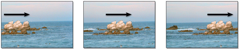
Figure 14.1
Image translating from left to right
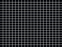
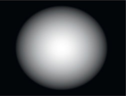
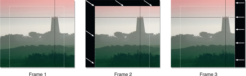
Some software packages offer a “wraparound” option for their translation operations. The pixels that get pushed out of frame on one side will “wrap around” to be seen on the other side of the frame. One of the main uses of a wraparound feature is with a paint program. By blending away the seam in a wrapped-around image, a “tile” can be made that can be used repeatedly to seamlessly tile a region.
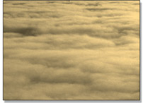
Figure 14.2
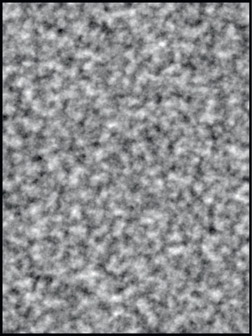
Original
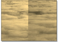
Figure 14.3
Wraparound
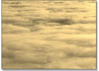
Figure 14.4
Blended
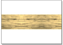
Figure 14.5
Tiled
Figure 14.2 shows an original cloud image. In Figure 14.3 it has been translated half its width in wraparound mode which created a seam down the middle of the picture. The seam has been blended away in Figure 14.4 using a paint program then the resulting image scaled down and tiled three times horizontally in Figure 14.5. If you took the blended image in Figure 14.4 and wrapped it around vertically and painted out the horizontal seam you would have an image that could be tiled infinitely both horizontally and vertically.
14.1.1.1.1 Float vs. Integer Translation
You may find that your software offers two different translate operations, one that is integer and one that is floating point. The integer version may go by another name, such as “pixel shift”. The difference is that the integer version can only position the image on exact pixel boundaries, such as moving it by exactly 100 pixels in X. The floating-point version, however, can move the image by any fractional amount, such as 100.73 pixels in X.
The integer version should never be used in animation because the picture would “hop” from pixel to pixel with a jerky motion. For animation the floating-point version is the only choice because it can move the picture smoothly at any speed to any position. The integer version, however, is the tool of choice if you need to simply reposition a plate to a new fixed location. The integer operation will not soften the image with filtering operations like the floating-point version will. The softening of images due to filtering is discussed in Section 14.1.4: Filtering. However, if you only have a floating-point type of transform but carefully enter integer values and do not animate them you can avoid any filtering.
14.1.1.1.2 Source and Destination Movement
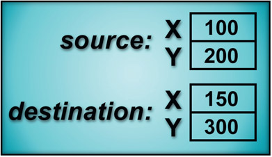
Figure 14.6
Source and destination type translate
With some software packages you just enter the amount to translate the image in X and Y and off it goes. We might call these “absolute” translate operations. Others have a source and destination type format, which is a “relative” translate operation. An example is shown in Figure 14.6. The relative translate operation is a bit more obtuse but can be more useful, as we will see in the image-stabilizing and difference-tracking operations later. The source and destination values work by moving the point that is located at source X,Y to the position located at destination X,Y, dragging the whole image with it, of course. In the example in Figure 14.6 the point at source location 100, 200 will be moved to destination location 150, 300. This means that the image will move 50 pixels in X and 100 pixels in Y. It is also true that if the source were 1100, 1200 and the destination were 1150, 1300 it would still move 50 pixels in X and 100 pixels in Y. In other words, the image is moved the relative distance from the source to the destination. So what good is all this source and destination relative positioning stuff?
Suppose you wanted to move an image from point A to point B. With the absolute translate you have to do the arithmetic yourself to find how much to move the image. You will get out your calculator and subtract the X position of point A from the X position of point B to get the absolute movement in X, then subtract the Y position of point A from the Y position of point B to get the absolute movement in Y. You may now enter your numbers in the absolute translate node and move your picture. With the relative translate node, you simply enter the X and Y position of point A as the source, then the X and Y position of point B as the destination, and off you go. The computer does all the arithmetic, which, I believe, is why computers were invented in the first place.
14.1.1.2 Rotation
Rotation appears to be the only image-processing operation in history to have been spared multiple names, so it will undoubtedly appear as “rotation” in your software. Most rotation operations are described in terms of degrees, so no discussion is needed here unless you would like to be reminded that 360 degrees makes a full circle. However, you may encounter a software package that refers to rotation in radians, a more sophisticated and elitist unit of rotation for the true trigonometry enthusiast.
While very handy for calculating the length of an arc section on the perimeter of a circle, radians are not an intuitive form of angular measurement when the mission is to straighten a tilted image. What you would probably really like to know is how big a radian is so that you can enter a plausible starting value and avoid whip-sawing the image around as you grope your way towards the desired angle. One radian is roughly 60 degrees. For somewhat greater precision, here is the official conversion between degrees and radians:
360 degrees = 2π radians
Not very helpful, was it. Two pi radians might be equal to 360 degrees, but you are still half a dozen calculator strokes away from any useful information. Table 14.1 contains a few pre-calculated reference points that you may actually find useful when confronted with a radian rotator:
Table 14.1 Converting degrees and radians
| radians to degrees | degrees to radians |
| 1 radian @ 57.3 degrees | 10 degrees @ 0.17 radians |
| 0.1 radian @ 5.7 degrees | 90 degrees @ 1.57 radians |
At least now you know that if you want to tilt your picture by a couple of degrees it will be somewhere around 0.03 radians. Since 90 degrees is about 1.57 radians, then 180 degrees must be about 3.14 radians. You are now cleared to solo with radian rotators.
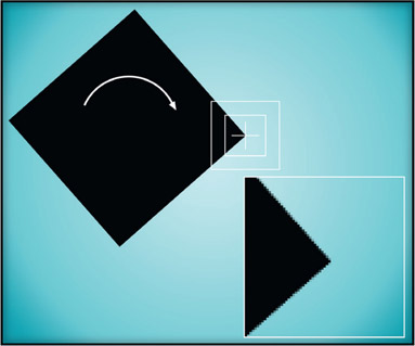
14.1.1.2.1 Pivot Points
Rotate operations have a “pivot point”, the point that is the center of the rotation operation. The location of the pivot point dramatically affects the results of the transform, so it is important to know where it is, its effects on the rotation operation, and how to reposition it when necessary.
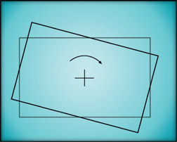
Figure 14.7
Centered pivot point
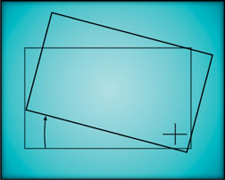
Figure 14.8
Off-center pivot point
The rotated rectangle in Figure 14.7 has its pivot point at its center so the results of the rotation are completely intuitive. In Figure 14.8, however, the pivot point is down in the lower right-hand corner and the results of the rotation operation are quite different. The degree of rotation is identical between the two rectangles, but the final position has been shifted up and to the right by comparison. Rotating an object about an off-center pivot point also displaces it in space. If the pivot point were placed far enough away from the rectangle it could have actually rotated completely out of frame!
14.1.1.3 Resize vs. Scale
Scaling, resizing, and zooming are tragically interchangeable terms in many software packages. Regardless of the terminology, there are two possible ways that these operations can behave. A “scale” or “resize” operation most often means that the size of the image changes while the composition of the picture is unchanged, like the examples in Figure 14.9. Going forward we will use the unambiguous term “resize” for this type of transform.
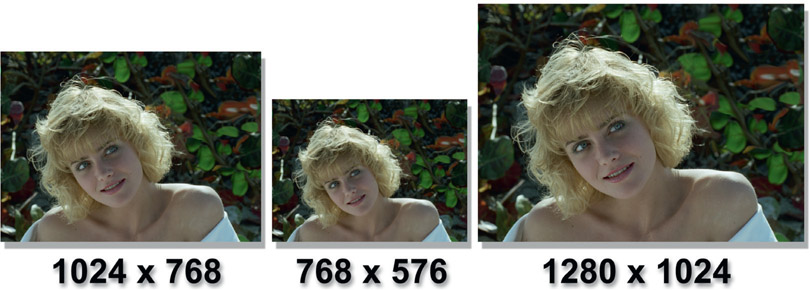
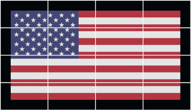
Figure 14.9
Image resize operation: image size changes but composition stays constant
A “zoom” or “scale” most often means that the image stays the same dimensions in X and Y, but the picture within it changes framing to become larger or smaller as though the camera were zoomed in or out like the example in Figure 14.10. Going forward we will use the term “scale” for this type of transform.

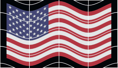
Figure 14.10
Image scale operation: image size stays constant but composition changes
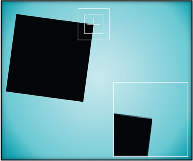
14.1.1.3.1 Pivot Points
The resize operation does not have a pivot point because it simply changes the dimensions of the image in X and Y. The scale operation, however, is like rotation, in that it must have a center about which the scale operation occurs, which is also referred to as the pivot point.
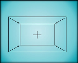
Figure 14.11
Centered pivot point
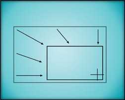
Figure 14.12
Off-center pivot point
The scaled rectangle in Figure 14.11 has its pivot point at the center of the outline so the results of the scale are not surprising. In Figure 14.12, however, the pivot point is down in the lower right-hand corner and the results of the scale operation are quite different. The amount of scale is identical with Figure 14.11, but the final position of the rectangle has been shifted down and to the right. Scaling an object about an off-center pivot point also displaces it in space. Again, if the pivot point were to be placed far enough away from an object it could actually scale itself completely out of the frame.
14.1.1.4 Skew

Figure 14.13
Horizontal and vertical skews
The overall shape of an image may also be deformed with a skew or “shear”, like the examples in Figure 14.13. The skew shifts one edge of the image relative to its opposite edge: the top edge of the image relative to the bottom edge in a horizontal skew, or the left and right edges in a vertical skew. Some systems will use one edge as the pivot point, others will use the images pivot point for the skew. The skew is occasionally useful for deforming a matte or alpha channel to be used as a shadow on the ground, but corner pinning will give you more control over the shadow’s shape and allow the introduction of perspective as well.
14.1.1.5 Corner Pinning

Figure 14.14
Corner pinning examples
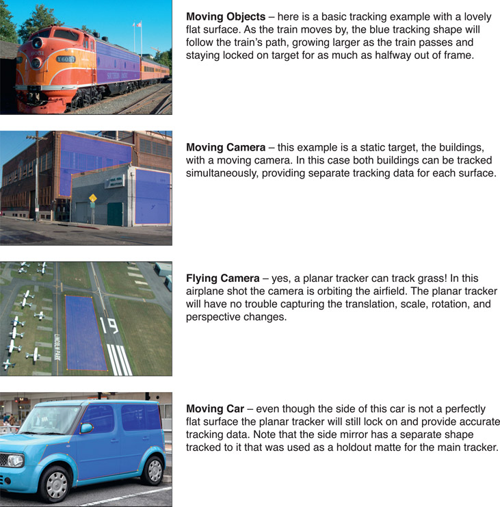
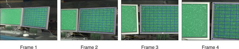
Corner pinning, shown in Figure 14.14, is an important image deformation tool because it allows you to arbitrarily alter the overall shape of an image. This is especially useful when the element you want to add to a shot isn’t exactly the right shape, or needs a subtle perspective shift. The image can be deformed as if it were mounted on a sheet of rubber where any or all of the four corners can be moved in any direction. The arrows in Figure 14.14 show the direction each corner point was moved in each example. The corner locations can also be animated over time so that the perspective change can follow a moving target in a motion-tracking application such as a monitor insert shot. A corner pin exactly matches the perspective shift you would get if the image were placed on a 3D card and re-photographed with a 3D camera, because 3D cameras uses a “pinhole” camera model with no lens distortion. Real cameras add lens distortion so would not exactly match a corner pin deformation.
Always keep in mind that corner pinning does not actually change the perspective in the image content itself. The only way that the perspective can really be changed is to view the original scene from a different camera position. All corner pinning can do is deform the image plane that the picture is on, which can appear as a fairly convincing perspective change – if it isn’t pushed too far.
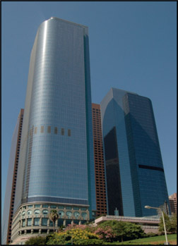
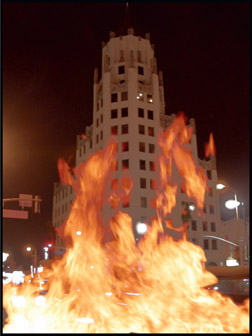
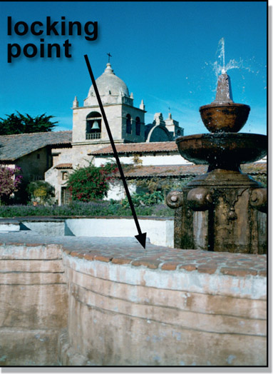
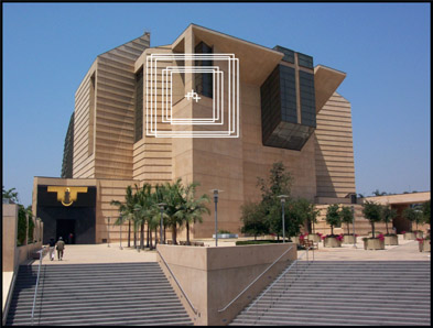
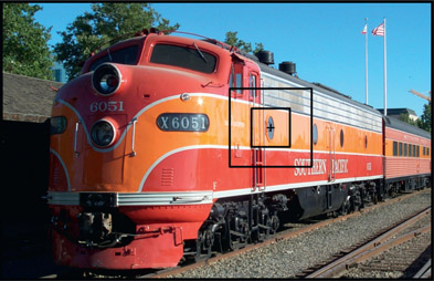
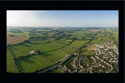
Figure 14.15
Original image
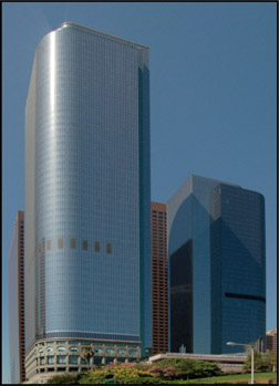
Figure 14.16
Perspective removed
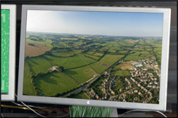
An example of a perspective change can be seen starting with Figure 14.15. The building was shot at an up-angle from a distance away so the picture has a noticeable perspective that tapers the building inwards at the top. Figure 14.16 shows the taper taken out of the building by stretching the two top corners apart with corner pinning. The perspective change makes the building appear as though it were shot from a greater distance with a longer lens. Unless you look closely, that is. There are still a few clues in the picture that reveal the camera distance if you know what to look for, but the casual observer won’t notice them, especially if the picture is only on screen briefly.
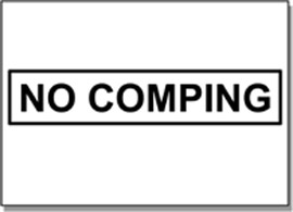
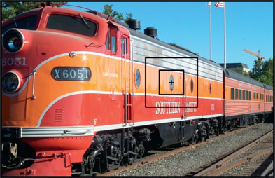
Figure 14.17
Original graphic

Figure 14.18
Original background

Figure 14.19
Corner pin perspective
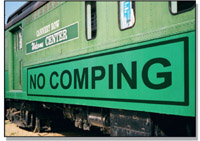
Figure 14.20
Perspective graphic on background
Another application of the corner pin perspective change is to lay an element on top of a flat surface, which is illustrated from Figure 14.17 to Figure 14.20. The sign graphic in Figure 14.17 is to be added to the side of the railroad car in Figure 14.18. The sign graphic has been deformed with four-corner pinning in Figure 14.19 to match the perspective. In Figure 14.20 the sign has been comped over the railroad car and now looks like it belongs in the scene.
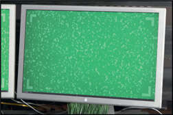
Corner pinning is really big in monitor insert shots. Motion tracking tools are used to track all four corners of the monitor then that tracking data is applied to the four corners of a corner pin operation. The corner pinned element will then track on the target monitor and change perspective over the length of the shot. This technique is used to place pictures on monitors and TV sets instead of trying to film them on the set.
WWW Corner Pin – this folder contains the two images shown in Figure 14.17 and Figure 14.18 above, so you too can try your hand at corner pinning the “no comping” graphic onto the railcar.
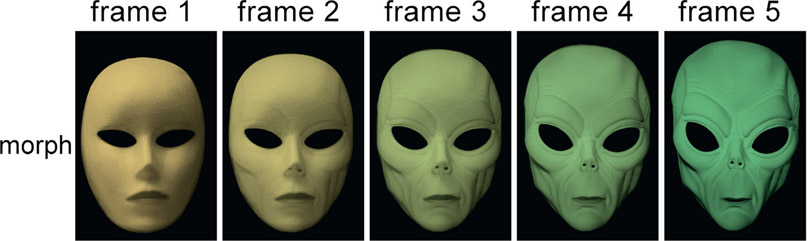
14.1.2 Managing Motion Blur

Figure 14.21
Photographic motion blur
If an object moves while the camera shutter is open the resulting image will be “smeared” in the direction of motion. This motion blur is an essential component of moving pictures because without it the motion will appear jerky with what is called “motion judder” or “motion strobing”. An object will become motion blurred if it moves fast enough but the entire frame will be motion-blurred if the camera itself is moved quickly enough.
The modern digital compositor is expected to manage the motion blur of a shot, and that can mean a couple things. If you add motion to a static element (a still image) then you will have to give it an appropriate motion blur. If you do a speed change, the motion blur from the original shot may be unsuitable for the new speed-changed version.
14.1.2.1 Transform Motion Blur
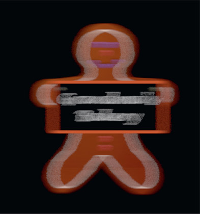
Figure 14.22
Stochastic motion blur
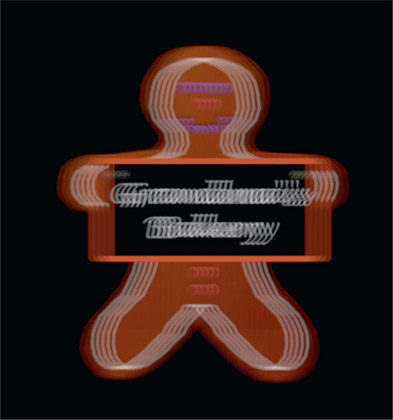
Figure 14.23
Multi-copy motion blur
Transform motion blur is when the transform operation that moved the item can itself add motion blur, and there are two types. Figure 14.22 illustrates a stochastic motion blur, which generates motion-blurred pixels using a random (stochastic) pattern. It turns out that this is actually more visually appealing than a perfectly uniform motion blur. The multi-copy type of motion blur in Figure 14.23 essentially just stamps a series of semi-transparent copies on top of each other. It is somewhat less convincing but computationally cheaper.
Your transform motion blur will hopefully have motion blur with two parameters you can adjust – quality and quantity. The quality parameter affects how computationally expensive the motion blur is since higher quality means more samples, which requires more computing. The quantity parameter is how “long” the motion blur is – that is, how much it smears the image. This is actually a shutter parameter because the longer you leave the shutter open the more the image moves and the more motion blur it gets. The shutter parameter may also have a “phase” option that allows you to advance or retard the shutter timing, which moves the motion blur forward or backward from its center.
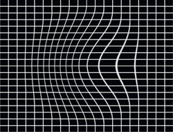
14.1.2.2 Motion UV Motion Blur
Rendering a CGI object with motion blur is very expensive, so a far less expensive 2D motion-blur technique is often used instead. One of the AOVs (Arbitrary Output Variables) that the CGI renderer can generate is a motion UV pass. The idea is that for each RGB pixel rendered, a two-channel pixel is also generated that contains the information on how that pixel is moving relative to the screen. If, for example, the RGB pixel were moving to the right 1.4 pixels and up by 0.3 pixels on that frame, then the motion UV pixel would contain 1.4 in the U channel and 0.3 in the V channel. This motion UV data has several uses, and one of them is to apply an inexpensive 2D motion blur in compositing.
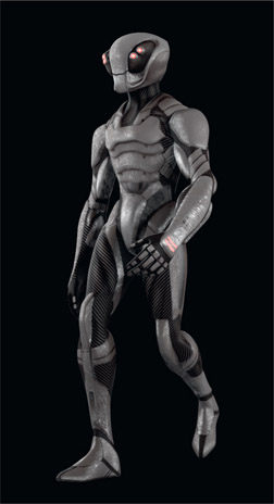
Figure 14.24
Original image
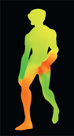
Figure 14.25
Motion UV pass
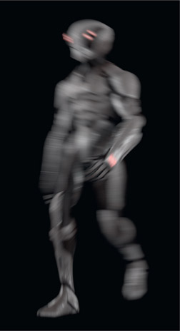
Figure 14.26
Motion-blurred image
Figure 14.24 shows a freshly rendered CGI character and Figure 14.25 shows the two-channel motion UV data for that frame. To make the motion data visible it has been normalized to between 0 and 1.0 and the UV data has been loaded into the viewer’s red and green channels. The motion UV data is piped to a vector-blur operation that applies the actual blur to the CGI render like the example in Figure 14.26, which is somewhat overdone for illustration purposes. Note that each part of the character is motion-blurred in a unique direction based on its own local motion. Those parts that are not moving on this frame, like the right foot and left hand, have no motion blur at all.
A true 3D motion blur would give somewhat better results but would be far more expensive and require the re-render of all of the lighting and AOV passes just to refine the motion blur, because it affects all of the lighting passes. In an age where one frame of high-end CGI for a feature film could take 24 hours PER FRAME to render this is a vastly cheaper and more practical alternative.
In this example the motion UV data from a CGI render provided the motion data to a vector blur operation but it is entirely possible to use this same technique for live action. The key is to be able to produce high quality motion data from the live action, which can be done by specialized motion analysis software.
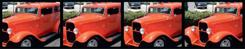
14.1.2.3 Speed Changes
Another motion-blur management opportunity arises with speed changes, which we do often in visual effects. The basic problem is that when the clip was initially photographed the motion blur was baked into the frames. If the clip is sped up it should have more motion blur than the initial photography but if slowed down it should have less.
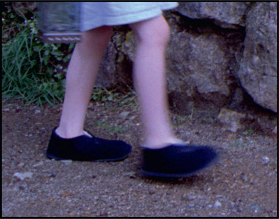
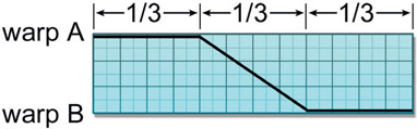
Figure 14.27
Original motion blur
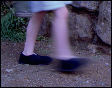
Figure 14.28
Increased motion blur from speed change
So how do we change the motion blur of a running clip? The answer is that it is done in your own excellent speed-change software. Figure 14.27 shows the original motion blur captured during principal photography. The clip was sped up by a factor of 10 in Figure 14.28 and the speed-change software, under the nuanced guidance of a talented vfx artist, has introduced an appropriate amount of motion blur for the much faster speed. The speed-changed clip needs to be inspected at full speed by a practiced eye to make sure the new motion blur is appropriate for the new speed.
14.1.3 3D Transforms
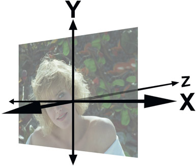
Figure 14.29
Three-dimensional axes
3D transforms are so named because the image behaves as though it exists in three dimensions. You can think of it as though the picture were placed on a card and the card can then be rotated, translated and scaled in any direction then rendered with a new perspective. The traditional placement of the three-dimensional axes are shown in Figure 14.29. The X axis goes left to right, the Y axis up and down, and the Z axis is perpendicular to the screen, going into the picture.
If an image is translated in X it will move left and right. If it is rotated in X (rotated about the X axis) it will rotate like the example in Figure 14.30. If the image is translated in Y it will move vertically. If it is rotated in Y it will rotate like the example in Figure 14.31. When translated in Z the image will get larger or smaller like a zoom as it moves towards or away from the “camera”. When rotated around Z it appears to rotate like a conventional 2D rotation. The 3D transform node will have rotate, scale, and translate operations in the same node so that they can all be choreographed together with one set of motion curves.
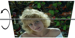
Figure 14.30
Rotate in X

Figure 14.31
Rotate in Y
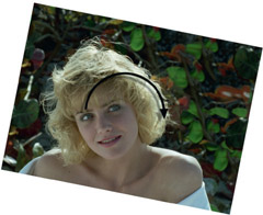
Figure 14.32
Rotate in Z
The time to use 3D transforms is when you want to “fly” something around the screen. Take a simple example like flying a logo in from the upper corner of the screen. The logo needs to translate from the corner of the screen to the center, and at the same time zoom from small to large. Coordinating these two movements so that they look natural together using conventional 2D scales and translations is tough. This is because the problem is in reality a three-dimensional problem and you are trying to fake it with separate two-dimensional tools. Better to use a 3D transform node to perform a true 3D move on the logo.
14.1.4 Filtering
Whenever an image goes through a transform its pixels are resampled, or “filtered” to create the pixels for the new version of the image. These filtering operations soften the image, degrading its sharpness. Therefore an understanding of how they work and which ones to use under what circumstances can be very important. Your professional compositing software will allow you to choose which filter to use for the resampling.
14.1.4.1 The Effects of Filtering
The filtering operation will soften the image because the new version is created by blending together percentages of adjacent pixels to create each new pixel. This is an irreversible degradation of the image. If you rotate an image a few degrees then rotate it back, it will not return to its original sharpness.

Figure 14.33
Original image

Figure 14.34
Rotation

Figure 14.35
Translation
An example can be seen starting with an extreme close-up of a small rectangular detail in the original image in Figure 14.33. It has a one-pixel border of anti-aliasing pixels at the outset. In Figure 14.34 the image has been rotated 5 degrees and the resampled pixels can be seen all around the perimeter. Figure 14.35 illustrates a simple floating-point translation of the original image and shows how the edge pixels have become further blurred by the filtering operation. Of course, scaling an image up softens it even more because in addition to the filtering operation you have fewer pixels to spread out over more picture space.
If you have stacked up several transforms on an image and the softening becomes objectionable, see if you have a multi-function transform operation that has all (or most) of the transforms incorporated in one. These operators concatenate all of the different transforms (rotate, scale, translate) into a single operation, so the amount of softening is greatly reduce because the image is only filtered once. Some professional software will concatenate multiple separate transform operations automatically if they are adjacent. However, if you insert a non-transform operation such as a color correction between them you will break the concatenation and suffer multiple filtering hits. Check your manual.
Simple pixel shift operations do not soften the image because they don’t filter. The pixels are just picked up and placed into their new location without any processing. Of course, this makes it an integer operation, which should never be used for animation but is fine for the overall repositioning of a background plate. The one case where filtering does not soften the image is when scaling an image down. Here the pixels are still being filtered, but they are also being squeezed down into a smaller image space so it tends to sharpen the whole picture. In film work, the scaled-down image could become so sharp that it actually needs to be softened to match the rest of the shot.
14.1.4.2 Twinkling Starfields
One situation where pixel filtering commonly causes problems is the “twinkling starfield” phenomenon. You’ve created a lovely starfield and then you go to animate it – either rotating it or perhaps translating it around – only to discover that the stars are twinkling! Their brightness is fluctuating during the move for some mysterious reason, and when the move stops, the twinkling stops.
What’s happening is that the stars are very small, only 1 or 2 pixels in size, and when they are animated they become filtered with the surrounding black pixels. If a given star were to land on an exact pixel location, it might retain its original brightness. If it landed on the “crack” between two pixels it might be averaged across them and drop to 50% brightness on each pixel. The brightness of the star then fluctuates depending on where it lands each frame, thus twinkling as it moves.
So what’s the fix? Bigger stars, I’m afraid. The basic problem is that the stars are at or very near the size of a pixel, so they become badly hammered by the filtering operation. Make a starfield that is twice the size needed for the shot so that the stars are 2 or 3 pixels in diameter. Perform the motion on the oversized starfield, then size it down for the shot. With the stars several pixels in diameter they are much more resistant to the effects of being filtered with the surrounding black.
14.1.4.3 Choosing a Filter
There are a variety of filters that have been developed for pixel resampling, each with its own virtues and vices. Some of the more common ones are listed here, but you should read your user guide to know what your software provides. The better software packages will allow you to choose the most appropriate filter for your transform operations. The internal mathematical workings of the filters are not described since that is a ponderous and ultimately unhelpful topic for the compositor. The effects of the filter and its most appropriate application is offered instead.
Bicubic – high-quality filter for scaling images up. It actually incorporates an edge-sharpening process so the scaled up image doesn’t go soft so quickly. Under some conditions the edge-sharpening operation can introduce “ringing” artifacts that degrade the results. Most appropriate use is reformatting images up in size or scaling up.
Bilinear – simple filter for scaling images up or down. Runs faster than the bicubic because it uses simpler math and has no edge-sharpening. As a result images get soft sooner. Best use is for scaling images down, since it does not sharpen edges.
Gaussian – another high-quality filter for scaling images up. It does not have an edge-sharpening process. As a result, the output images are not as sharp, but they also do not have any ringing artifacts. Most appropriate use is to substitute for the Mitchell filter when it introduces ringing artifacts.
Impulse – a.k.a. “nearest neighbor”, a very fast, very low-quality filter. Not really a filter, it just “pixel plucks” from the source image – that is, it simply selects the nearest appropriate pixel from the source image to be used in the output image. This filter is commonly used for the viewer in compositing packages because it is fast. It will look fine on photographic images (except for very fine details) but when you put in graphics the deficiencies become apparent. Most appropriate use is for quickly making lower resolution motion test of a shot.
Mitchell – a type of bicubic filter where the filtering parameters have been dialed in for the best look on most images. Also does edge sharpening, but less prone to edge artifacts as a plain bicubic filter. Most appropriate use is to replace bicubic filter when it introduces edge artifacts.
Sinc – a special high quality filter for downsizing images. Other filters tend to lose small details or introduce aliasing when scaling down. This filter retains small details with good anti-aliasing. Most appropriate use is for scaling images down or zooming out.
Lanczos – high-quality filter for sizing images up or down with sharpening. It is considered the best compromise in terms of reducing aliasing, sharpness, with minimal ringing artifacts.
Triangle – simple filter for scaling images up or down. Runs faster than the sharpening filters because it uses simpler math and has no edge-sharpening. As a result, up-sized images get soft sooner. Best use is for scaling images down quickly since it does not sharpen edges.
14.1.5 Lining Up Images
It often comes to pass that you need to precisely line up one image on top of another. Most compositing packages offer some kind of “A/B” image comparison capability that can be helpful for lineup. Two images are loaded into a display window, then you can wipe or toggle between them to check and correct their alignment. This approach can be adequate for many situations, but there are times when you really want to see both images simultaneously rather than wiping or toggling between them.
The problem becomes trying to see what you are doing, since one layer covers the other. A simple 50% dissolve between the two layers (aka “onionskin”) is hopelessly confusing to look at, and overlaying the layers while wiping between them with one hand while you nudge their positions with the other is slow and awkward. What is really needed is some way of displaying both images simultaneously that still keeps them visually distinguished while you nudge them into position. Two different lineup display methods are offered here that will help you to do just that.
14.1.5.1 Offset Mask Lineup Display
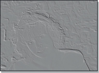
Figure 14.36
Embossed effect from offset images
The offset mask method combines two images in such a way that if the images are not perfectly aligned an embossed outline shows up like the example in Figure 14.36. The embossing marks all pixels that are not identical between the two images. If they are exactly lined up on each other the embossing disappears and it becomes a featureless gray image.
To make an offset mask simply invert one of the two images, then mix them together in equal amounts. This can be done with a dissolve node or a mix node set to 50%. To use discrete nodes, scale each image’s RGB values by 50% then add them together. A pictographic flowgraph of the whole process is shown in Figure 14.37. A good way to familiarize yourself with this procedure is to use the same image for both input images until you are comfortable that you have it set up right and can “read” the signs of misalignment. Once set up correctly, substitute the real image to be lined up for one of the inputs.
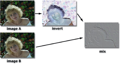
Figure 14.37
Pictographic flowgraph for making an offset mask
Once set up, the procedure is to simply reposition one of the images until the offset mask becomes a uniform gray in the region you want lined up. While this is a very precise “offset detector” that will reveal the slightest difference between the two images, it suffers from the drawback that it does not directly tell you which way to move which image to line the two up. It simply indicates that they are not perfectly aligned. Of course, you can experimen-tally slide the image in one direction, and if the embossing gets worse, go back the other way. With a little practice you should become clear which image is which.
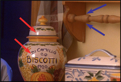
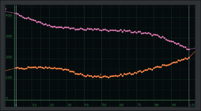
14.1.5.2 Edge-detection Lineup Display
Lineup method number two is the edge-detection method. The beauty of this method is that it makes it perfectly clear which image to move and in what direction to achieve the lineup. The basic idea is to use an edge-detection operation on a monochrome version of the two images to make an “outline” version of each. One outline is placed in the red channel, the other in the green channel, and the blue channel is filled with black, as shown in the flowgraph in Figure 14.38. When the red and green outline images are correctly lined up on each other, the lines turn yellow. If they slide off from each other, you see red lines and green lines again which tell you exactly how far and in what direction to move in order to line them up. You will see shortly why I like to put the image that needs to be moved in the green channel.
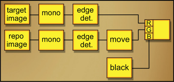
Figure 14.38 Flowgraph of lineup edges
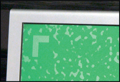
Examples of this lineup method can be seen in Figure 14.39 through Figure 14.42. They show the monochrome image and its edge-detection version, then how the colors change when the edges are misaligned (Figure 14.41) vs. aligned (Figure 14.42).

Figure 14.39
Grayscale image

Figure 14.40
Edge detection
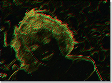
Figure 14.41
Images offset

Figure 14.42
Images aligned
One of the difficulties of an image-lineup procedure is trying to stay clear in your mind as to which image is being moved and in what direction. You have an image being repositioned (the repo image) and a reference image that you are trying to line it up to. If you will put the reference image in the red channel and the repo image in the green channel like the flowgraph in Figure 14.38, then you can just remember the little mnemonic “move the green to the red”. Since the color green is associated with “go” and the color red with “stop” for traffic lights, it is easy to stay clear on what is being moved (green) vs. what is the static reference (red). This method makes it easier to see what you are doing, but it can be less precise than the offset mask method described above.
14.1.5.3 The Pivot Point Lineup Procedure
Now that we have a couple of good ways to see what we are doing when we want to line up two images, this is a good time to discuss an efficient method of achieving the actual lineup itself. The effects of the pivot-point location can be used to excellent advantage when trying to line up two elements that are dissimilar in size, position, and orientation. It can take quite a bit of trial and error in scaling, positioning, rotating, repositioning, rescaling, repositioning, etc. to get two elements lined up. By using a strategically placed pivot point and the procedure in Figure 14.43 (opposite) a complex lineup can be done quickly without all of the trial and error.

Figure 14.43 Pivot point lineup procedure