8.1 A Short Course in 3D
3D compositing has a great many terms and concepts that will be foreign to a straight up 2D compositor, which will make learning about it very difficult. In this section we pause for a short course in 3D to build up the vocabulary a compositor will need to take on 3D compositing. Again, 3D is a huge subject so we will only be covering those topics that are relevant to 3D compositing.
8.1.1 The 3D Coordinate System
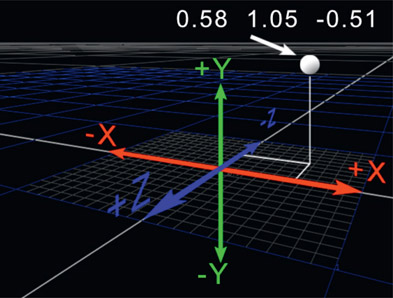
Figure 8.1
3D coordinate system
Most 2D compositors already understand 3D coordinate systems but it would be good to do a quick review to lock in a few key concepts and establish some naming conventions. Figure 8.1 shows a typical 3D coordinate system used by most 3D programs. Y is vertical, with positive Y being up. X is horizontal, with positive X being to the right. Z is towards and away from the screen with positive Z being towards the screen and negative Z being away.
Any point in 3D space (often referred to as “world space”) is located using three floating-point numbers that represent its position in X, Y, and Z. The white dot in Figure 8.1 is located at 0.58 (in X) 1.05 (in Y) and –0.51 (in Z) and is written as a triplet like this: 0.58 1.05 –0.51.
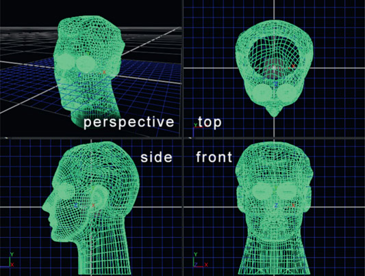
Figure 8.2 Perspective and orthogonal views
The 3D viewing part of the compositing system will present two types of views of the 3D world (Figure 8.2), perspective and orthogonal, which means “perpendicular”. The perspective view is as seen through a camera viewer while the orthogonal views can be thought of as “straight on” to the 3D geometry with no camera perspective. These “ortho” views are essential for precisely lining things up. The orthogonal view will further offer three versions: the top, front, and side views. If you have ever taken a drafting class in school this will all be very familiar. If you are the purely artistic type then this will all be quite unnatural, having no perspective and all.
8.1.2 Vertices
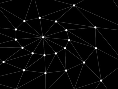
Figure 8.3
Vertices and polygons
Vertices (or the singular “vertex”) are the 3D points that define the surface of the geometry. In fact, 3D geometry is a list of vertices and a description of how they are connected – i.e. vertex numbers 1, 2 and 3 are connected to form a triangle, or a “polygon”. Figure 8.3 shows a series of vertices and how they are connected to create polygons. Polygons are joined together to form surfaces and surfaces are joined together to form objects.
8.1.3 Meshes
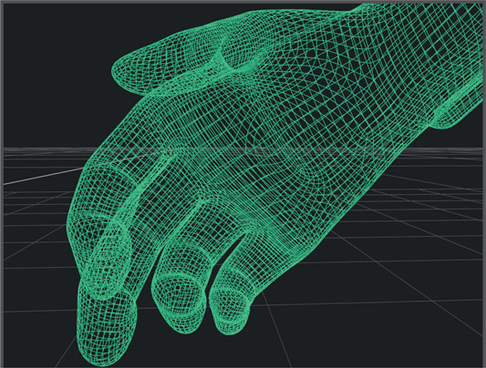
Figure 8.4
The mesh for a 3D hand
When the vertices are connected to define a 3D object the resulting geometry is referred to as a polygonal mesh, or just a mesh. This is the basic form in which complex compound curved objects such as characters or cars are represented in 3D systems such as Maya. In the 3D system the mesh is attached to an articulate “rig” that is actually a jointed skeleton. The 3D animator moves the skeleton and the skeleton moves the mesh.
These meshes can be “baked out” of the 3D system then imported into 3D compositing software. When baked out they lose their “skeletons” and can no longer be articulated but they can be resized and repositioned and even retimed – if working with Alembic geometry. More on this later.
8.1.4 Surface Normals
Surface normals are also key players in rendering CGI and 2D compositing. Rendering is the process of calculating the output image, based on the 3D geometry, surface attributes, camera, and lights. The brightness of a surface depends on its angle to the light source, so the surface normals are a necessary part of the calculation to determine their brightness. We saw a great use for surface normals in Chapter 7: Compositing CGI, to completely relight a CGI render from the 2D images. Consider Figure 8.5, the flat shaded surface. Each polygon has been rendered as a simple flat shaded element but the key point here is how each polygon is a slightly different brightness compared to its neighbor. Each polygon’s brightness is calculated based on the angle of its surface relative to the light source. If it is perpendicular to the light it is bright, but if it is at an angle it is rendered darker. It is the surface normal that is used to calculate this angle to the light so it is a fundamental player in the appearance of all 3D objects.
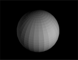
Figure 8.5 Flat shaded surface
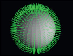
Figure 8.6
Surface normal
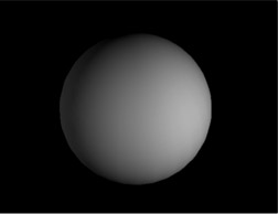
Figure 8.7
Smooth shaded surface
The sphere in Figure 8.6 is displayed with its surface normals visible. A surface normal is a vector, or little “arrow”, with its base in the center of the polygon face and pointing out perpendicular to its surface. The technical term when one object is perpendicular to another is to say that it is “normal” to that surface. So the surface normals are vectors that are perpendicular to the flat face of each polygon and are essential to computing its brightness. If the surface normals are smoothly interpolated across the surface of the geometry we can simulate a smooth shaded surface like the one shown in Figure 8.7. Note that this is really a rendering trick because the surface looks smooth and continuous when it is not. In fact, if you look closely you can still see the short straight segments of the sphere’s polygons around its outside edge.
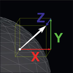
Figure 8.8
A surface normal
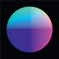
Figure 8.9
Surface normals in 3-channel image
In the world of compositing, the surface normal vectors are turned into 2D images that we can use for image processing. How this is done is illustrated starting in Figure 8.8, which shows a surface normal (white arrow). The base is at the center of a polygon and the arrow tip indicates in what direction it points rel ative to its base. The tip’s direction can be quantified by 3 numbers indicated by the X, Y and Z arrows, which measure the tip’s positional offset relative to its base. We can take these three numbers for each pixel and place them in a 3-channel image, like the example in Figure 8.9, such that the X data is stored in the red channel, Y in the green channel, and Z in blue. In other words, we have an “image” that does not contain a picture but rather data about the picture. We now have the 3D vector information shown in Figure 8.6 converted to the 2D form that we can use in compositing for a multitude of purposes.
8.1.5 UV Coordinates
Texture mapping is the process of wrapping pictures around 3D geometry like the example in Figure 8.10 and Figure 8.11. The name is a bit odd, however. If you actually want to add a texture to a 3D object (such as tree bark) you use another image called a bump map. So bump maps add texture, and texture maps add pictures. Oh well.
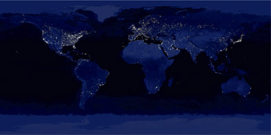
Figure 8.10
Texture map
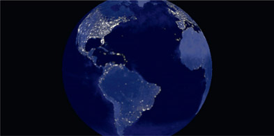
Figure 8.11
Texture map projected onto geometry
Actually, there are many different kinds of maps that can be applied to 3D geometry. A reflection map puts reflections on a surface. A reflectance map will create shiny and dull regions on the surface that will show more or less of the reflection, and so on. But we are not here to talk about the different kinds of maps that can be applied to geometry, for they are numerous and varied. We are here to talk about how they are all applied to the geometry, for that is a universal concept and what UV coordinates are all about.
The UV coordinates determine how a texture map is fitted onto the geometry. We could not use x and y for this because it is already taken, so the u coordinate is the horizontal axis and v is the vertical axis of the image. Each vertex in the geometry is assigned a UV coordinate that links that vertex to a specific point in the texture map. Since there is some distance between the vertices in the geometry the remaining parts of the texture map are estimated or “interpolated” to fill in between the actual vertices. Changing the UV coordinates of the geometry will reposition the texture map on its surface. There are many different methods of assigning the UV coordinates to the geometry and this process is called “map projection”.
8.1.6 Map Projection
Map projection is the process of fitting the texture map to geometry by assigning UV coordinates to its vertices. It is called “projection” because the texture map starts out as a flat 2D image and to wrap it around the geometry requires it to be “projected” into 3D space. There are a wide variety of ways to project a texture map onto 3D geometry and the key is to select a projection method that suits the shape of the geometry. Some common projections are planar, spherical, and cylindrical.
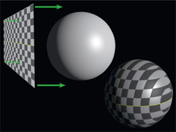
Figure 8.12 Planar projection

Figure 8.13
Spherical projection

Figure 8.14
Cylindrical projection
Figure 8.12 shows a planar projection of the texture map onto a sphere. You can think of a planar projection as walking face-first into a sticky sheet of Saran Wrap (yikes!). As you can see by the final textured sphere this projection method does not fit well so it stretches and streaks parts of the texture map. A planar projection would be the right choice if you were projecting a texture to the flat front of a building, for example.
Figure 8.13 shows a more promising approach to the sphere called spherical projection. You can think of this as stretching the texture map into a sphere around the geometry then shrink-wrapping it down in all directions. The key here is that the projection method matches the shape of the geometry.
Figure 8.14 shows a cylindrical projection of the texture map onto a sphere. Clearly a cylindrical projection was designed to project a texture map around cylinders, such as a can of soup, not a sphere. But this example demonstrates how the texture map is distorted when the projection method does not match the shape of the geometry.
8.1.7 UV Projection
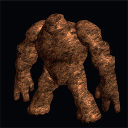
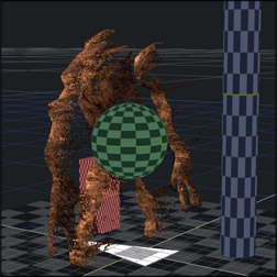
Simple geometry shapes can have their maps projected by simple rules but what about a complex compound curved surface like the wireframe character in Figure 8.15? No simple rule will do. For this kind of complex object a technique called UV projection is used. The texture map is painted on a dedicated 3D paint program designed for this type of work resulting in the confusing texture map in Figure 8.16. But the 3D geometry knows where all the bits go and the results are shown in Figure 8.17.

Figure 8.15 Wireframe geometry

Figure 8.16
Texture map
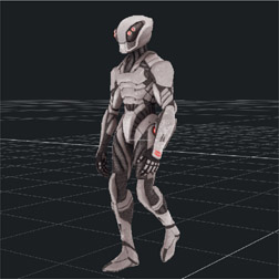
Figure 8.17
Texture map applied to geometry
To understand the confusing texture map in Figure 8.16 we need to understand how the texture map pixels get located onto the 3D geometry. As mentioned above, the texture map has horizontal coordinates labeled “u” (or “U”) and vertical coordinates labeled “v” (or “V”). Any pixel in the texture map can then be located by its UV coordinates. Unsurprisingly there are no firm industry standards, but many systems assign the UV coordinate 0,0 to the lower left corner and 1,1 to the upper right corner of the texture map. So a pixel in the dead center would have UV coordinates of 0.5, 0.5. The basic idea is somehow to assign the UV coordinate of 0.5, 0.5 to a particular vertex of the 3D geometry. This is the job of the 3D texture-painting program.
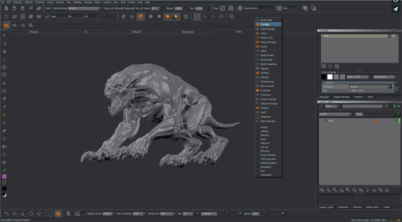
Figure 8.18
The awesome Mari 3D texture painting program
Figure 8.18 is a screen grab of Mari, a very powerful 3D texture-painting program by The Foundry, the makers of Nuke. The 3D geometry is loaded into Mari and the artist paints directly on the geometry. As the paint is applied Mari knows what vertex is under the paint brush, as well as the UV coordinate of the paint pixels it is generating, so it is building the UV list for the geometry as it is painted. The geometry is saved out of Mari with its freshly assigned UV coordinates and the texture map is saved out as an image file like EXR. While the appearance of the texture map image to humans is a bit confusing (see Figure 8.16) to the computer it makes perfect sense. Thanks to the 3D texture-painting program the 3D system knows exactly where to place every pixel of the texture map.
8.1.8 3D Geometry
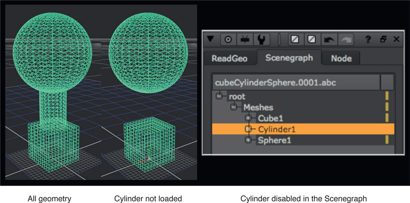
Generally speaking, we do not create the 3D geometry when doing 3D compositing. After all, we have to leave something for the 3D department to do, right? However, we often do need to use simple 3D shapes to project our texture maps so 3D compositing programs come with a small library of “geometric primitives”, which are simple 3D shapes. Figure 8.19 shows a lineup of the usual suspects – a plane, a cube, a sphere, and a cylinder. More complex 3D objects such as the character in Figure 8.15 are modeled in the 3D department then saved out in a file format that can then be read into the 3D compositing program.
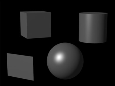
Figure 8.19
Geometric primitives
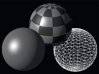
Figure 8.20
Solid, textured, and wireframe displays
Figure 8.20 shows how the geometry may also be displayed in three different ways. Solid, where the geometry is rendered with simple lighting only; textured, with texture maps applied; and wireframe. The reason for three different presentations is system response time. 3D is computationally expensive (slow to compute) and if you have a million-polygon database (not that unusual!) then you can wait a long time for the screen to update when you make a change. In wireframe mode the screen will update the quickest. If your workstation has the power or the database is not too large you might switch the 3D viewer to solid display. And of course, the textured display is slowest of all, but also the coolest.
8.1.9 Geometric Transformations
2D images can be transformed in a variety of ways – translate, rotate, scale, etc. which is explored in detail in Chapter 14: Transforms and Tracking. Of course, 3D objects can be transformed in the same ways. However, in the 2D world the transformation of an image is rarely dependent on or related to the transformation of other images. In the 3D world the transformation of one piece of geometry is very often hierarchically linked to the transformation of another. And it can quickly get quite complex and confusing.
There is one item that would be unfamiliar to a 2D compositor and that is the “null object”. A null object, or axis, is a 3-dimensional pivot point that you can create and assign to 3D objects, including lights and camera. In 2D you can shift the pivot point of an image, but you cannot create a new pivot point in isolation. In 3D it is done all the time.
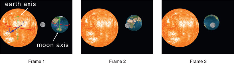
Figure 8.21
Axis for earth and moon added for animation
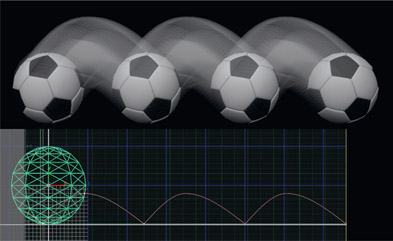
A typical example can be seen in the animation shown in the three frames of Figure 8.21. The Earth must both rotate and orbit around the Sun. The rotate is easily achieved by rotating the sphere around its own pivot point. However, to achieve the orbit around the Sun it needs a separate axis (null object) located at the Sun’s center. The Moon has exactly the same requirement so it too needs a separate axis to orbit around.
WWW Geometric transformations.mov – view the entire animation used for Figure 8.21 and see the axis in action for the Sun, Moon, and Earth.
8.1.10 Geometric Deformations
One thing you will be asked to do to your 3D geometry is to deform it. Maybe you need an ellipse rather than a sphere. Deform the sphere. Maybe the 3D geometry you loaded does not quite fit the live action correctly. Deform it to fit better. There are a great many ways to deform geometry, and they vary from program to program. But here are three fundamental techniques that will likely be in any 3D compositing program you encounter.
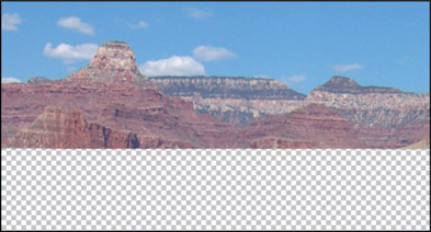
8.1.10.1 Image Displacement
Image displacement is definitely one of the coolest tricks in all of 3D-dom (displacement just means to shift something’s position). Simply take an image (see Figure 8.22), lay it down on top of a flat card that has been subdivided into many polygons and command the image to displace (shift) the vertices vertically based on the brightness of the image at each vertex. The result looks like the displaced geometry in Figure 8.22. The bright parts of the image have lifted the vertices up and the dark parts dropped them down resulting in a contoured piece of terrain. Just add a moving camera and render to taste.

Figure 8.22
Image displacement example
Figure 8.23 shows three frames out of an animation sequence rendered from Figure 8.22. If the camera were simply to slide over the original flat image that is exactly what it would look like – a flat image moving in front of the camera. With image displacement, the variation in height creates parallax and it appears as real terrain with depth variations. You can see what I mean with the movie provided on the website below. And it is very photo-realistic because it uses a photograph. Talk about cheap thrills. Besides terrain, this technique can be used to make clouds, water, and many other 3D effects.
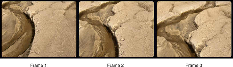
Figure 8.23 Frames from camera flyover displaced terrain
In this example the same image was used for both the displacement map and the texture map. Sometimes a separate image is painted for the displacement map to control it more precisely, and the photograph is used only as the texture map.
WWW Image displacement.mov – this video shows the really cool terrain fly-over created by the simple image displacement shown in Figure 8.23.
8.1.10.2 Noise displacement

Figure 8.24
Geometry displaced with noise
Instead of using an image to displace geometry we can also use “noise” – mathematically generated noise or turbulence. In our 2D world we use 2D noise so in the 3D world we have 3D noise. There also tends to be a greater selection of the types of noise, as well as a greater sophistication of the controls.
Figure 8.24 illustrates a flat piece of subdivided geometry that has been displaced in Y with a robust Perlin noise function. This can be a very efficient (cheap) way to generate acres of terrain. These noise and turbulence functions can also be animated to make clouds or water – perhaps water seen from a great distance.
WWW Noise displacement.mov – this video is an animation showing the use of noise displacement shown in Figure 8.24. Caution – it’s a bit freaky.
8.1.10.3 Deformation Lattice
The third and final geometric deformation example is the deformation lattice. The concept is to place the geometry inside of a bounding box called a “deformation lattice”, then deform the lattice. The geometry inside the lattice is deformed accordingly. We can see an example starting with the original geometry in Figure 8.25. The deformation lattice is shown surrounding the geometry in Figure 8.26. Note that some programs have more subdivisions and control points than the simple example shown here. The artist then moves the control points at the corners of the lattice and the geometry inside is deformed proportionally as shown in Figure 8.27.
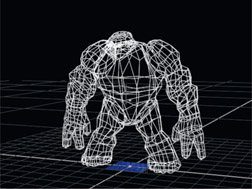
Figure 8.25
Original geometry
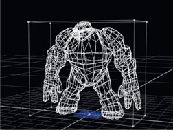
Figure 8.26
Deformation lattice added

Figure 8.27
Deformed geometry
While this example shows an extreme deformation in order to illustrate the process, the main use in the real world of 3D compositing is to make small overall adjustments to the shape of the geometry when it doesn’t quite fit right in the scene.
WWW Deformation lattice.mov – this video shows the deformation lattice from Figure 8.27 in action.
8.1.11 Point Clouds
Point clouds are another form of 3D geometry that consist of… a cloud of points. The idea is that we want to represent a 3D object or scene but we don’t have a polygonal model to see a smooth shaded or texture mapped version of it. They are a far lighter load for the computer and are easily moved around the screen in real-time. But how are they made and what are they used for?
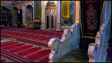
Figure 8.28
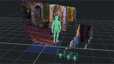
Live action clip with camera move
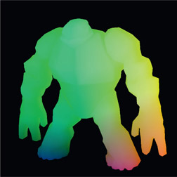
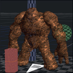
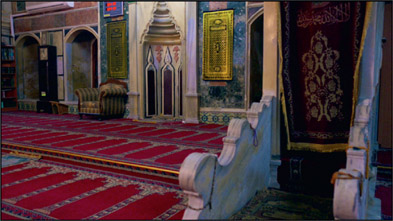
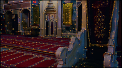
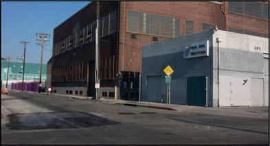
Point clouds come from two sources. Most commonly they are produced by a 3D camera tracker that tracked a scene then the artist asked for a point cloud to be generated that represents the surfaces in the scene (see Section 8.4: Camera Tracking). The second source is Lidar (Light Detection And Ranging), which uses a laser to scan a scene to collect location data for millions of points. Figure 8.28 shows a live action clip that was camera tracked to produce the colored point cloud in Figure 8.29.
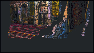
Figure 8.29
Point cloud from same POV
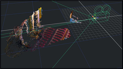
Figure 8.30
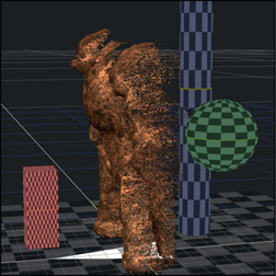
Point cloud with camera
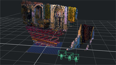
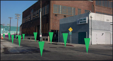
The point cloud is being viewed through the solved camera so it’s being viewed from the same POV as the original live action clip. Figure 8.30 shows the point cloud and solved camera from a different POV. What’s important to note here is what is missing. There are “voids” in the point cloud caused by the fact that the camera didn’t get a good enough look at those areas to calculate a point for it. For camera tracking to produce a 3D point the camera has to be moving and view it from several different angles over several frames. Points with insufficient coverage are discarded, which leaves the voids.
As for what point clouds are good for, they are used primarily to line up 3D elements for a 3D composting scene. Figure 8.29, for example, could be used to place a 3D object on the floor such as a character walking across the room. Most high-end compositing programs have a built-in camera tracker so compositors can generate their own point clouds and “solved cameras” for their 3D compositing shots (the reverse engineered camera and lens is referred to as the “solved camera”).
WWW Point cloud.mov – this movie will give you an orbiting camera view of the point cloud shown in Figure 8.29. You can see how this would be very handy for placing 3D geometry to photograph with the “solved camera”.
8.1.12 Lights
3D lights are one of the key features common to all 3D compositing programs. They can be located and pointed in 3D space, animated, their brightness adjusted, and even a color tint added. Many even have a falloff setting so the light will get dimmer with distance. Just like the real world.
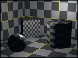
Figure 8.31
Point light

Figure 8.32
Spotlight
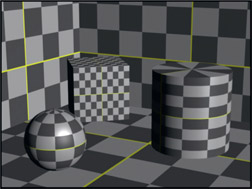
Figure 8.33
Parallel light
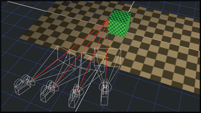
Here are the three basic types of lights you are sure to encounter in a 3D compositing program. Figure 8.31 shows a point light, which is like a single bare bulb hanging in the middle of our little 3D “set”. Unlike the real world, 3D lights themselves are never seen because the program does not render them as visible objects. It only renders the effect of the light they emit. Figure 8.32 is a spotlight that is parked off to the right with its adjustable cone aimed at the set. Figure 8.33 is a parallel light that simulates the parallel light rays from a light source at a great distance, like the Sun, streaming in from the right.
Note the lack of shadows. Casting shadows is a computationally expensive feature and is typically reserved for real 3D software. Note also that the computer simulated “light rays” pass right through the 3D objects and will illuminate things that should not be lit, such as the inside of a mouth.
Because 3D lights are virtual and mathematical you can get clever and darken the inside of the mouth by hanging a light inside of it, then give it a negative brightness so it “radiates darkness”. This is perfectly legal in the virtual world of 3D.
8.1.13 Shaders
After the 3D geometry is created the type of surface it represents must be defined. Is it a hard shiny surface like plastic? Is it a dull matte surface like a pool table? In fact, the surface of 3D geometry can have multiple layers of attributes and these are created by shaders. Shaders are a hugely complex subject manned by towering specialists whose sole job is to create and refine them. In fact, they are called shader writers and are highly paid specialists in the world of CGI.
The shaders in a 3D compositing program will be simple and require no programming, but you will have to adjust their parameters to get realistic surface attributes on your geometry. Here we will take a look at three basic shaders – ambient, diffuse, and specular. Each example shows three intensity levels from dark to bright to help show the effect of the shader. Note that these intensity changes are achieved by increasing the shader values, not by increasing the light source. In the virtual world of CGI you can increase the brightness of objects by either making the light brighter or dialing up the shader. Or both.
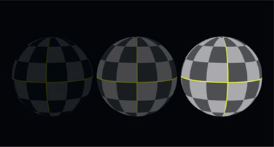
Figure 8.34
Ambient shader

Figure 8.35
Diffuse shader
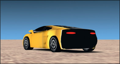
Starting with the ambient shader in Figure 8.34, it simply causes the 3D object to emit light from every pore and is unaffected by any lights. It can be used in two ways. First, it is used to add a low level of ambient light to prevent unlit areas of the geometry from rendering as zero black. Second, by cranking an ambient shader way up it becomes a self-illuminated object, such as the taillight of a car. However, it does not cast any light on other objects. It just gets brighter itself.
Figure 8.35 shows the effect of a diffuse shader, which definitely responds to lights. If you increase the brightness of the light the geometry will get brighter. The diffuse shader darkens the polygons as they turn away from the light source. It uses the surface normals we saw earlier to determine how perpendicular the polygon is to the light source, and then calculates its brightness accordingly.
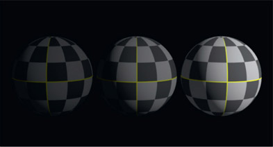
Figure 8.36
Ambient plus diffuse
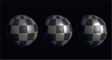
Figure 8.37
Specular added
One key concept about shaders is that they can be summed together to build up surface complexity. Figure 8.36 shows the combination of the ambient plus the diffuse shaders at three intensity levels. Figure 8.37 shows the middle sample from Figure 8.36 with three different intensities of a specular shader added to make it look progressively shinier. Again, there are no changes in the light source, just the shader.
8.1.14 Reflection Mapping
Reflection mapping is an amazing photo-realistic 3D lighting technique that does not use any 3D lights at all. Instead, the entire scene is illuminated with a special photograph taken on the set or on location. This photograph is then (conceptually) wrapped around the entire 3D scene as if on a bubble at infinite distance, then the reflection map is seen on any reflective surface. This is not light projected into the 3D scene, it is just reflections on shiny objects.
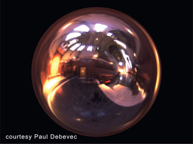
Figure 8.38
A light probe image
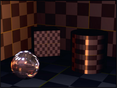
Figure 8.39
Scene illuminated with reflection map only
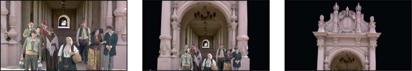
Figure 8.38 shows a light probe image, that “special photograph” mentioned above, taken on location. This particular location being the interior of a cathedral. Figure 8.39 is our little 3D set with some degree of reflectivity enabled for all the geometry. No 3D lights were used. It is as if these objects were built in a model shop then set down on the floor in the actual cathedral.
There are two specific requirements to make the bizarre photograph in Figure 8.38 work as an environment light. The first is that it must be a High Dynamic Range (HDR) image, and the second is that it is a 360-degree photograph made with a “light probe”, a highly reflective chrome sphere. Of course, it needs to be a reasonably high-resolution image as well. The light probe is placed at the center of the location then photographed so the camera sees the entire environment as if it were in the center of the room photographing in all directions at once – minus the scene content obscured by the light probe itself.
This particular image captures the lights in the room as well as the windows with sunlight streaming in at their true brightness levels so that they can then “shine” on the 3D objects in the scene. Of course, the image is badly distorted spherically, but this is trivial for a computer to unwrap back into the original scene – which is exactly what is done as part of the reflection mapping process.
WWW Reflection map.mov – check out this video showing the light probe in Figure 8.38 as a reflection map around a rotating chrome bust. There are no lights, just a reflection map.
8.1.15 Ray Tracing
You may recall from Section 8.1.12: Lights that we had a little problem with shadows – namely that there weren’t any. That’s because computing shadows takes more work – a lot more work – than simply calculating how bright each polygon is. Note that the scenes in Figure 8.31 to Figure 8.33 are rendered as though the light were passing right through the objects and falling onto the surfaces behind them. That’s because it is. The simple scan-line render algorithm used here just looks at each surface in isolation relative to its light source. If we want to improve the accuracy of the render to reflect more correctly what real light rays would do in a real scene we have to up our game and switch to ray tracing.

Figure 8.40
Ray tracing is required for reflections and refractions
Consider the complex image in Figure 8.40. To render images like this, light rays are traced throughout the scene including all the reflections and refractions. Surprisingly, the ray-tracing process starts at the viewing screen and traces light rays backwards into the scene. For each pixel, a ray is traced into the scene until it hits its first surface, then depending on the nature of that surface, it may bounce away and out of the picture or bounce to another object or even refract through some glass and strike something in the background. Some will stop cold when they hit a non-reflective opaque surface thus casting a shadow behind the object. So ray tracing is how high quality shadows, reflections and refractions are generated. However, there are some cheats to save computing time that will generate pretty good shadows without the expense of a ray tracer, which you may find in your 3D compositing software.
The thing to appreciate about ray tracing is how incredibly expensive it is. When rendering a 2k-frame for example, we start with the fact that there are over two million pixels at the viewing screen, so we will have two million rays to trace. In reality multiple rays are cast per pixel to avoid aliasing, but that’s another story. The point is these millions of rays are bouncing all over the scene interacting multiple times with multiple surfaces, so the entire process entails billions, sometimes trillions of calculations. But it sure looks nice.
8.1.16 Image-Based Lighting
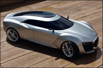
Figure 8.41
Photorealism with image-based lighting
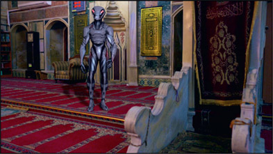
The latest trend in CGI rendering techniques is Image-Based Lighting (IBL), which produces astonishingly photorealistic images like the one in Figure 8.41. IBL is actually an extension of the reflection mapping we saw in Section 8.1.14: Reflection Mapping above that used a light probe to capture a 360-degree HDR image of the scene, then used that to generate reflections off of shiny objects. Only in this case the image is actually used as the light source for the scene. The beauty of this approach is that it produces astonishing photorealistic CGI scenes. But of course, it too is computationally expensive.

Figure 8.42
Light probe
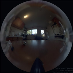
Figure 8.43
Exposure lowered
Figure 8.42 shows the type of light-probe photo used to illuminate scenes like Figure 8.41 which in this case just happens to be a photo of a kitchen. The light probe need not really be from the actual scene in question just as long as it has useful light sources. The room content can be masked off so that just the light sources are used to illuminate the scene and the light probe can be rotated around to position the light source wherever needed. Beyond being an HDR image they must also be very high resolution, perhaps 10k or better. Note that the light probe image is not a very pretty picture. It’s not intended to be. It is intended to be a data capture of the scene illumination all the way up to the brightest light sources, hence the HDR. Figure 8.43 illustrates the enormous dynamic range in the photo by knocking the exposure way down so the bright light sources become visible. You can see the ceiling kitchen light and the windows with sky outside. These will become the actual light sources for illuminating the 3D objects in a scene. IBL is often used when a 3D scene needs to be modeled on a real location. They will take their light probe and HDR camera to the original scene to capture the local lighting, then use that to light the 3D model of the scene. Very photorealistic.
8.1.17 Cameras
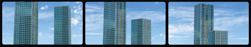
After the geometry, texture maps, and lights are all in place, the next thing we will need to photograph our 3D scene is a camera. 3D cameras work virtually like the real thing (sorry about that “virtually”) with an aperture, focal length (zoom) position in 3D space, and orientation (rotate in X, Y, Z). And of course, all of these parameters can be animated over time. Figure 8.44 illustrates a time-lapse exposure of a moving 3D camera in a scene. A very powerful feature of 3D cameras is that not only can the compositor animate them, but camera data from either the 3D department or the matchmove department can be imported into the compositing software so that our 3D compositing camera exactly matches the cameras in the 3D department or the live action world. This is an immensely important feature and is at the heart of much 3D compositing work.
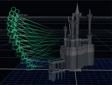
Figure 8.44
Animated 3D camera
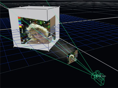
Figure 8.45
Camera projection
An important difference between 3D cameras and real-world cameras is that the 3D camera does not introduce lens distortion to its images but live action cameras with real lenses do. This adds a whole layer of issues when mixing live action with 3D scenes, whether it is in the 3D department or the compositing department. There is a detailed treatment of this important topic in Chapter 11: Camera Effects.
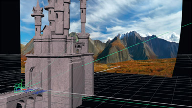
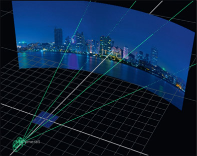
One totally cool trick a 3D camera can do that a real one cannot is a technique called “camera projection”. In this application the camera is turned into a virtual slide projector then pointed at any 3D geometry. Any image in the camera is then projected onto the geometry like the illustration in Figure 8.45. If a movie clip (a scene) is placed in the camera then the clip can be projected onto the geometry. Camera projection is a bit like walking around your office with a running film projector shining it on various objects in the room. It is a very powerful and oft-used technique in 3D compositing and we will see a compelling example of its use shortly.