Substituting the identities E[Xn]=1,E[Xn2]=2 in the preceding shows that

E[Sn]=n+n2/2

and the induction proof is complete. (c) If we let Cj denote the number of hats chosen by person j,j=1,…,n then

∑j=1nCj=Sn

Taking expectations, and using the fact that each Cj has the same mean, yields the result

E[Cj]=E[Sn]/n=1+n/2

Hence, the expected number of false selections by person j is

E[Cj-1]=n/2.■

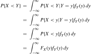
Example 3.15

Independent trials, each of which is a success with probability p, are performed until there are k consecutive successes. What is the mean number of necessary trials?

Solution: Let Nk denote the number of necessary trials to obtain k consecutive successes, and let Mk=E[Nk]. We will determine Mk by deriving and then solving a recursive equation that it satisfies. To begin, write

Nk=Nk-1+Ak-1,k

where Nk-1 is the number of trials needed for k-1 consecutive successes, and Ak-1,k is the number of additional trials needed to go from having k-1 successes in a row to having k in a row. Taking expectations gives that,

Mk=Mk-1+E[Ak-1,k]

To determine E[Ak-1,k], condition on the next trial after there have been k-1 successes in a row. If it is a success then that gives k in a row and no additional trials after that are needed; if it is a failure then at that point we are starting all over and so the expected addtional number from then on would be E[Nk]. Thus,

E[Ak-1,k]=1·p+(1+Mk)(1-p)=1+(1-p)Mk

giving that

Mk=Mk-1+1+(1-p)Mk

or

Mk=1p+Mk-1p

Since N1, the time of the first success, is geometric with parameter p, we see that

M1=1p

and, recursively

M2=1p+1p2,M3=1p+1p2+1p3

and, in general,

Mk=1p+1p2+⋯+1pk■

Example 3.16

Analyzing the Quick-Sort Algorithm

Suppose we are given a set of n distinct values—x1,…,xn—and we desire to put these values in increasing order or, as it is commonly called, to sort them. An efficient procedure for accomplishing this is the quick-sort algorithm, which is defined recursively as follows: When n=2 the algorithm compares the two values and puts them in the appropriate order. When n>2 it starts by choosing at random one of the n values—say, xi—and then compares each of the other n-1 values with xi, noting which are smaller and which are larger than xi. Letting Si denote the set of elements smaller than xi, and S¯i the set of elements greater than xi, the algorithm now sorts the set Si and the set S¯i. The final ordering, therefore, consists of the ordered set of the elements in Si, then xi, and then the ordered set of the elements in S¯i. For instance, suppose that the set of elements is 10, 5, 8, 2, 1, 4, 7. We start by choosing one of these values at random (that is, each of the 7 values has probability of 17 of being chosen). Suppose, for instance, that the value 4 is chosen. We then compare 4 with each of the other six values to obtain

{2,1},4,{10,5,8,7}

We now sort the set {2, 1} to obtain

1,2,4,{10,5,8,7}

Next we choose a value at random from {10,5,8,7}—say 7 is chosen—and compare each of the other three values with 7 to obtain

1,2,4,5,7,{10,8}

Finally, we sort {10,8} to end up with

1,2,4,5,7,8,10

One measure of the effectiveness of this algorithm is the expected number of comparisons that it makes. Let us denote by Mn the expected number of comparisons needed by the quick-sort algorithm to sort a set of n distinct values. To obtain a recursion for Mn we condition on the rank of the initial value selected to obtain

Mn=∑j=1nE[number of comparisons∣value selected isjth smallest]1n

Now, if the initial value selected is the jth smallest, then the set of values smaller than it is of size j-1, and the set of values greater than it is of size n-j. Hence, as n-1 comparisons with the initial value chosen must be made, we see that

Mn=∑j=1n(n-1+Mj-1+Mn-j)1n=n-1+2n∑k=1n-1Mk(sinceM0=0)

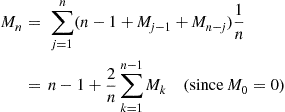
or, equivalently,

nMn=n(n-1)+2∑k=1n-1Mk

To solve the preceding, note that upon replacing n by n+1 we obtain

(n+1)Mn+1=(n+1)n+2∑k=1nMk

Hence, upon subtraction,

(n+1)Mn+1-nMn=2n+2Mn

or

(n+1)Mn+1=(n+2)Mn+2n

Therefore,

Mn+1n+2=2n(n+1)(n+2)+Mnn+1

Iterating this gives

Mn+1n+2=2n(n+1)(n+2)+2(n-1)n(n+1)+Mn-1n=⋯=2∑k=0n-1n-k(n+1-k)(n+2-k)sinceM1=0

Hence,

Mn+1=2(n+2)∑k=0n-1n-k(n+1-k)(n+2-k)=2(n+2)∑i=1ni(i+1)(i+2),n⩾1

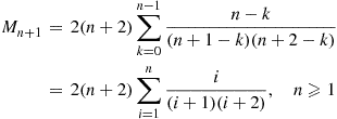
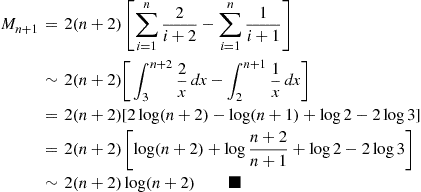
Using the identity i/(i+1)(i+2)=2/(i+2)-1/(i+1), we can approximate Mn+1 for large n as follows:

Mn+1=2(n+2)∑i=1n2i+2-∑i=1n1i+1∼2(n+2)∫3n+22xdx-∫2n+11xdx=2(n+2)[2log(n+2)-log(n+1)+log2-2log3]=2(n+2)log(n+2)+logn+2n+1+log2-2log3∼2(n+2)log(n+2)■

Although we usually employ the conditional expectation identity to more easily enable us to compute an unconditional expectation, in our next example we show how it can sometimes be used to obtain the conditional expectation.

Example 3.17

In the match problem of Example 2.31 involving n,n>1, individuals, find the conditional expected number of matches given that the first person did not have a match.

Solution: Let X denote the number of matches, and let X1 equal 1 if the first person has a match and 0 otherwise. Then,

E[X]=E[X∣X1=0]P{X1=0}+E[X∣X1=1]P{X1=1}=E[X∣X1=0]n-1n+E[X∣X1=1]1n

But, from Example 2.31

E[X]=1

Moreover, given that the first person has a match, the expected number of matches is equal to 1 plus the expected number of matches when n-1 people select among their own n-1 hats, showing that

E[X∣X1=1]=2

Therefore, we obtain the result

E[X∣X1=0]=n-2n-1■

3.4.1 Computing Variances by Conditioning

Conditional expectations can also be used to compute the variance of a random variable. Specifically, we can use

Var(X)=E[X2]-(E[X])2

and then use conditioning to obtain both E[X] and E[X2]. We illustrate this technique by determining the variance of a geometric random variable.

Example 3.18

Variance of the Geometric Random Variable

Independent trials, each resulting in a success with probability p, are performed in sequence. Let N be the trial number of the first success. Find Var(N).

Solution: Let Y=1 if the first trial results in a success, and Y=0 otherwise.

Var(N)=E[N2]-(E[N])2

To calculate E[N2] and E[N] we condition on Y. For instance,

E[N2]=EE[N2∣Y]

However,

E[N2∣Y=1]=1,E[N2∣Y=0]=E[(1+N)2]

These two equations are true since if the first trial results in a success, then clearly N=1 and so N2=1. On the other hand, if the first trial results in a failure, then the total number of trials necessary for the first success will equal one (the first trial that results in failure) plus the necessary number of additional trials. Since this latter quantity has the same distribution as N, we get that E[N2∣Y=0]=E[(1+N)2]. Hence, we see that

E[N2]=E[N2∣Y=1]P{Y=1}+E[N2∣Y=0]P{Y=0}=p+E[(1+N)2](1-p)=1+(1-p)E[2N+N2]

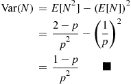
Since, as was shown in Example 3.10, E[N]=1/p, this yields

E[N2]=1+2(1-p)p+(1-p)E[N2]

or

E[N2]=2-pp2

Therefore,

Var(N)=E[N2]-(E[N])2=2-pp2-1p2=1-pp2■

Another way to use conditioning to obtain the variance of a random variable is to apply the conditional variance formula. The conditional variance of X given that Y=y is defined by

Var(X∣Y=y)=E(X-E[X∣Y=y])2∣Y=y

That is, the conditional variance is defined in exactly the same manner as the ordinary variance with the exception that all probabilities are determined conditional on the event that Y=y. Expanding the right side of the preceding and taking expectation term by term yields

Var(X∣Y=y)=E[X2∣Y=y]-(E[X∣Y=y])2

Letting Var(X∣Y) denote that function of Y whose value when Y=y is Var(X∣Y=y), we have the following result.

Proposition 3.1

The Conditional Variance Formula

Var(X)=EVar(X∣Y)+VarE[X∣Y] (3.7)

(3.7)

Proof

EVar(X∣Y)=E[E[X2∣Y]-(E[X∣Y])2]=EE[X2∣Y]-E(E[X∣Y])2=E[X2]-E(E[X∣Y])2

and

Var(E[X∣Y])=E(E[X∣Y])2-EE[X∣Y]2=E(E[X∣Y])2-(E[X])2

Therefore,

EVar(X∣Y)+VarE[X∣Y]=E[X2]-(E[X])2

which completes the proof. ■

Example 3.19

The Variance of a Compound Random Variable

Let X1,X2,… be independent and identically distributed random variables with distribution F having mean μ and variance σ2, and assume that they are independent of the nonnegative integer valued random variable N. As noted in Example 3.10, where its expected value was determined, the random variable S=∑i=1NXi is called a compound random variable. Find its variance.

Solution: Whereas we could obtain E[S2] by conditioning on N, let us instead use the conditional variance formula. Now,

Var(S∣N=n)=Var∑i=1NXi∣N=n=Var∑i=1nXi∣N=n=Var∑i=1nXi=nσ2

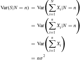
By the same reasoning,

E[S∣N=n]=nμ

Therefore,

Var(S∣N)=Nσ2,E[S∣N]=Nμ

and the conditional variance formula gives

Var(S)=E[Nσ2]+Var(Nμ)=σ2E[N]+μ2Var(N)

If N is a Poisson random variable, then S=∑i=1NXi is called a compound Poisson random variable. Because the variance of a Poisson random variable is equal to its mean, it follows that for a compound Poisson random variable having E[N]=λ

Var(S)=λσ2+λμ2=λE[X2]

where X has the distribution F. ■

Example 3.20

The Variance in the Matching Rounds Problem

Consider the matching rounds problem of Example 3.14, and let Vn=Var(Rn) denote the variance of the number of rounds needed when there are initially n people. Using the conditional variance formula, we will show that

Vn=n,n⩾2

The proof of the preceding is by induction on n. To begin, note that when n=2 the number of rounds needed is geometric with parameter p=1/2 and so

V2=1-pp2=2

So assume the induction hypothesis that

Vj=j,2⩽j<n

and now consider the case when there are n individuals. If X is the number of matches in the first round then, conditional on X, the number of rounds Rn is distributed as 1 plus the number of rounds needed when there are initially n-X individuals. Consequently,

E[Rn∣X]=1+E[Rn-X]=1+n-XbyExample 3.14

Also, with V0=0,

Var(Rn∣X)=Var(Rn-X)=Vn-X

Hence, by the conditional variance formula

Vn=E[Var(Rn∣X)]+Var(E[Rn∣X])=E[Vn-X]+Var(X)=∑j=0nVn-jP(X=j)+Var(X)=VnP(X=0)+∑j=1nVn-jP(X=j)+Var(X)

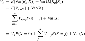
Because P(X=n-1)=0, it follows from the preceding and the induction hypothesis that

Vn=VnP(X=0)+∑j=1n(n-j)P(X=j)+Var(X)=VnP(X=0)+n(1-P(X=0))-E[X]+Var(X)

As it is easily shown (see Example 2.31 and Exercise 72 of Chapter 2) that E[X]=Var(X)=1, the preceding gives

Vn=VnP(X=0)+n(1-P(X=0))

thus proving the result. ■

3.5 Computing Probabilities by Conditioning

Not only can we obtain expectations by first conditioning on an appropriate random variable, but we may also use this approach to compute probabilities. To see this, let E denote an arbitrary event and define the indicator random variable X by

X=1,ifEoccurs0,ifEdoes not occur

It follows from the definition of X that

E[X]=P(E),E[X∣Y=y]=P(E∣Y=y),for any random variableY

Therefore, from Equations (3.2a) and (3.2b) we obtain

P(E)=∑yP(E∣Y=y)P(Y=y),ifYis discrete=∫-∞∞P(E∣Y=y)fY(y)dy,ifYis continuous

Example 3.21

Suppose that X and Y are independent continuous random variables having densities fX and fY, respectively. Compute P{X<Y}.

Solution: Conditioning on the value of Y yields

P{X<Y}=∫-∞∞P{X<Y∣Y=y}fY(y)dy=∫-∞∞P{X<y∣Y=y}fY(y)dy=∫-∞∞P{X<y}fY(y)dy=∫-∞∞FX(y)fY(y)dy

where

FX(y)=∫-∞yfX(x)dx■

Example 3.22

An insurance company supposes that the number of accidents that each of its policyholders will have in a year is Poisson distributed, with the mean of the Poisson depending on the policyholder. If the Poisson mean of a randomly chosen policyholder has a gamma distribution with density function

g(λ)=λe-λ,λ⩾0

what is the probability that a randomly chosen policyholder has exactly n accidents next year?

Solution: Let X denote the number of accidents that a randomly chosen policyholder has next year. Letting Y be the Poisson mean number of accidents for this policyholder, then conditioning on Y yields

P{X=n}=∫0∞P{X=n∣Y=λ}g(λ)dλ=∫0∞e-λλnn!λe-λdλ=1n!∫0∞λn+1e-2λdλ

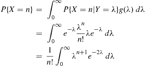
However, because

h(λ)=2e-2λ(2λ)n+1(n+1)!,λ>0

is the density function of a gamma (n+2,2) random variable, its integral is 1. Therefore,

1=∫0∞2e-2λ(2λ)n+1(n+1)!dλ=2n+2(n+1)!∫0∞λn+1e-2λdλ

showing that

P{X=n}=n+12n+2■

Example 3.23

Suppose that the number of people who visit a yoga studio each day is a Poisson random variable with mean λ. Suppose further that each person who visits is, independently, female with probability p or male with probability 1-p. Find the joint probability that exactly n women and m men visit the academy today.

Solution: Let N1 denote the number of women and N2 the number of men who visit the academy today. Also, let N=N1+N2 be the total number of people who visit. Conditioning on N gives

P{N1=n,N2=m}=∑i=0∞P{N1=n,N2=m∣N=i}P{N=i}

Because P{N1=n,N2=m∣N=i}=0 when i≠n+m, the preceding equation yields

P{N1=n,N2=m}=P{N1=n,N2=m∣N=n+m}e-λλn+m(n+m)!

Given that n+m people visit it follows, because each of these n+m is independently a woman with probability p, that the conditional probability that n of them are women (and m are men) is just the binomial probability of n successes in n+m trials. Therefore,

P{N1=n,N2=m}=n+mnpn(1-p)me-λλn+m(n+m)!=(n+m)!n!m!pn(1-p)me-λpe-λ(1-p)λnλm(n+m)!=e-λp(λp)nn!e-λ(1-p)(λ(1-p))mm!

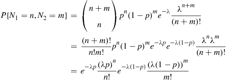
Because the preceding joint probability mass function factors into two products, one of which depends only on n and the other only on m, it follows that N1 and N2 are independent. Moreover, because

P{N1=n}=∑m=0∞P{N1=n,N2=m}=e-λp(λp)nn!∑m=0∞e-λ(1-p)(λ(1-p))mm!=e-λp(λp)nn!

and, similarly,

P{N2=m}=e-λ(1-p)(λ(1-p))mm!

we can conclude that N1 and N2 are independent Poisson random variables with respective means λp and λ(1-p). Therefore, this example establishes the important result that when each of a Poisson number of events is independently classified either as being type 1 with probability p or type 2 with probability 1-p, then the numbers of type 1 and type 2 events are independent Poisson random variables. ■

The result of Example 3.23 generalizes to the case where each of a Poisson distributed number of events, N, with mean λ is independently classified as being one of k types, with the probability that it is type i being pi,i=1,…,k,∑i=1kpi=1. If Ni is the number that are classified as type i, then N1,…,Nk are independent Poisson random variables with respective means λp1,…,λpk. This follows, since for n=∑i=1kni

P(N1=n1,…,Nk=nk)=P(N1=n1,…,Nk=nk∣N=n)P(N=n)=n!n1!⋯nk!p1n1⋯pknke-λλn/n!=∏i=1ke-λpi(λpi)ni/ni!

where the second equality used that, given a total of n events, the numbers of each type has a multinomial distribution with parameters (n,p1,…,pk).

Example 3.24

The Distribution of the Sum of Independent Bernoulli Random Variables

Let X1,…,Xn be independent Bernoulli random variables, with Xi having parameter pi,i=1,…,n. That is, P{Xi=1}=pi,P{Xi=0}=qi=1-pi. Suppose we want to compute the probability mass function of their sum, X1+⋯+Xn. To do so, we will recursively obtain the probability mass function of X1+⋯+Xk, first for k=1, then k=2, and on up to k=n. To begin, let

Pk(j)=P{X1+⋯+Xk=j}

and note that

Pk(k)=∏i=1kpi,Pk(0)=∏i=1kqi

For 0<j<k, conditioning on Xk yields the recursion

Pk(j)=P{X1+⋯+Xk=j∣Xk=1}pk+P{X1+⋯+Xk=j∣Xk=0}qk=P{X1+⋯+Xk-1=j-1∣Xk=1}pk+P{X1+⋯+Xk-1=j∣Xk=0}qk=P{X1+⋯+Xk-1=j-1}pk+P{X1+⋯+Xk-1=j}qk=pkPk-1(j-1)+qkPk-1(j)

Starting with P1(1)=p1,P1(0)=q1, the preceding equations can be recursively solved to obtain the functions P2(j),P3(j), up to Pn(j). ■

Example 3.25

The Best Prize Problem

Suppose that we are to be presented with n distinct prizes in sequence. After being presented with a prize we must immediately decide whether to accept it or reject it and consider the next prize. The only information we are given when deciding whether to accept a prize is the relative rank of that prize compared to ones already seen. That is, for instance, when the fifth prize is presented we learn how it compares with the first four prizes already seen. Suppose that once a prize is rejected it is lost, and that our objective is to maximize the probability of obtaining the best prize. Assuming that all n! orderings of the prizes are equally likely, how well can we do?

Solution: Rather surprisingly, we can do quite well. To see this, fix a value k,0⩽k<n, and consider the strategy that rejects the first k prizes and then accepts the first one that is better than all of those first k. Let Pk (best) denote the probability that the best prize is selected when this strategy is employed. To compute this probability, condition on X, the position of the best prize. This gives

Pk(best)=∑i=1nPk(best∣X=i)P(X=i)=1n∑i=1nPk(best∣X=i)

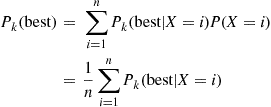
Now, if the overall best prize is among the first k, then no prize is ever selected under the strategy considered. On the other hand, if the best prize is in position i, where i>k, then the best prize will be selected if the best of the first k prizes is also the best of the first i-1 prizes (for then none of the prizes in positions k+1,k+2,…,i-1 would be selected). Hence, we see that

Pk(best∣X=i)=0,ifi⩽kPk(best∣X=i)=P{best of firsti-1is among the firstk}=k/(i-1),ifi>k

From the preceding, we obtain

Pk(best)=kn∑i=k+1n1i-1≈kn∫kn-11xdx=knlogn-1k≈knlognk

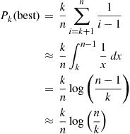
Now, if we consider the function

g(x)=xnlognx

then

g′(x)=1nlognx-1n

and so

g′(x)=0⇒log(n/x)=1⇒x=n/e