3.2 The Discrete Case
Recall that for any two events E and F
and F , the conditional probability of E
 given F
 is defined, as long as P(F)>0
 , by
, by
P(E∣F)=P(EF)P(F)
Hence, if X and Y
and Y are discrete random variables, then it is natural to define the conditional probability mass function of X
 given that Y=y
 , by
, by
pX∣Y(x∣y)=P{X=x∣Y=y}=P{X=x,Y=y}P{Y=y}=p(x,y)pY(y)
for all values of y such that P{Y=y}>0
 . Similarly, the conditional probability distribution function of X
 given that Y=y
 is defined, for all y
 such that P{Y=y}>0
 , by
, by
FX∣Y(x∣y)=P{X⩽x∣Y=y}=∑a⩽xpX∣Y(a∣y)
Finally, the conditional expectation of X given that Y=y
 is defined by
E[X∣Y=y]=∑xxP{X=x∣Y=y}=∑xxpX∣Y(x∣y)
In other words, the definitions are exactly as before with the exception that everything is now conditional on the event that Y=y . If X
 is independent of Y
 , then the conditional mass function, distribution, and expectation are the same as the unconditional ones. This follows, since if X
 is independent of Y
 , then
pX∣Y(x∣y)=P{X=x∣Y=y}=P{X=x}
Example 3.1
Suppose that p(x,y) , the joint probability mass function of X
 and Y
and Y , is given by
p(1,1)=0.5,p(1,2)=0.1,p(2,1)=0.1,p(2,2)=0.3
Calculate the conditional probability mass function of X given that Y=1
 .
.
Solution: We first note that
pY(1)=∑xp(x,1)=p(1,1)+p(2,1)=0.6
Hence,
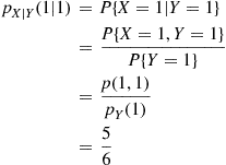
pX∣Y(1∣1)=P{X=1∣Y=1}=P{X=1,Y=1}P{Y=1}=p(1,1)pY(1)=56
Similarly,
pX∣Y(2∣1)=p(2,1)pY(1)=16■
Example 3.2
If X1 and X2
 are independent binomial random variables with respective parameters (n1,p)
 and (n2,p)
 , calculate the conditional probability mass function of X1
 given that X1+X2=m
 .
.
Solution: With q=1-p ,
,
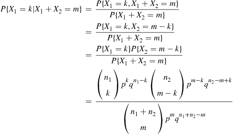
P{X1=k∣X1+X2=m}=P{X1=k,X1+X2=m}P{X1+X2=m}=P{X1=k,X2=m-k}P{X1+X2=m}=P{X1=k}P{X2=m-k}P{X1+X2=m}=n1kpkqn1-kn2m-kpm-kqn2-m+kn1+n2mpmqn1+n2-m
where we have used that X1+X2 is a binomial random variable with parameters (n1+n2,p)
 (see Example 2.44). Thus, the conditional probability mass function of X1
 , given that X1+X2=m
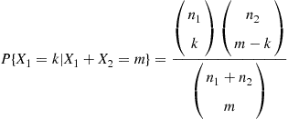
 , is
, is
P{X1=k∣X1+X2=m}=n1kn2m-kn1+n2m (3.1)
 (3.1)
(3.1)
The distribution given by Equation (3.1), first seen in Example 2.35, is known as the hypergeometric distribution. It is the distribution of the number of blue balls that are chosen when a sample of m balls is randomly chosen from an urn that contains n1
 blue and n2
 red balls. (To intuitively see why the conditional distribution is hypergeometric, consider n1+n2
 independent trials that each result in a success with probability p
 ; let X1
 represent the number of successes in the first n1
 trials and let X2
 represent the number of successes in the final n2
 trials. Because all trials have the same probability of being a success, each of the n1+n2m
 subsets of m
 trials is equally likely to be the success trials; thus, the number of the m
 success trials that are among the first n1
 trials is a hypergeometric random variable.) ■
Conditional expectations possess all of the properties of ordinary expectations. For example such identities such as
E∑i=1nXi∣Y=y=∑i=1nE[Xi∣Y=y]E[h(X)∣Y=y]=∑xh(x)P(X=x∣Y=y)
remain valid.
Example 3.4
There are n components. On a rainy day, component i
 will function with probability pi
 ; on a nonrainy day, component i
 will function with probability qi
 , for i=1,…,n
 . It will rain tomorrow with probability α
 . Calculate the conditional expected number of components that function tomorrow, given that it rains.
Solution: Let
Xi=1,if componentifunctions tomorrow0,otherwise
Then, with Y defined to equal 1 if it rains tomorrow, and 0 otherwise, the desired conditional expectation is obtained as follows.
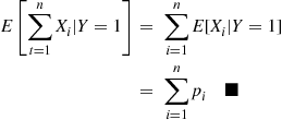
E∑t=1nXi∣Y=1=∑i=1nE[Xi∣Y=1]=∑i=1npi■
3.3 The Continuous Case
If X and Y
and Y have a joint probability density function f(x,y)
 , then the conditional probability density function of X
 , given that Y=y
 , is defined for all values of y
 such that fY(y)>0
 , by
, by
fX∣Y(x∣y)=f(x,y)fY(y)
To motivate this definition, multiply the left side by dx and the right side by (dxdy)/dy
 to get
fX∣Y(x∣y)dx=f(x,y)dxdyfY(y)dy≈P{x⩽X⩽x+dx,y⩽Y⩽y+dy}P{y⩽Y⩽y+dy}=P{x⩽X⩽x+dx∣y⩽Y⩽y+dy}
In other words, for small values dx and dy
 , fX∣Y(x∣y)dx
 is approximately the conditional probability that X
 is between x
 and x+dx
 given that Y
 is between y
 and y+dy
 .
.
The conditional expectation of X , given that Y=y
 , is defined for all values of y
 such that fY(y)>0
 , by
, by
E[X∣Y=y]=∫-∞∞xfX∣Y(x∣y)dx
Example 3.5
Suppose the joint density of X and Y
and Y is given by
f(x,y)=6xy(2-x-y),0<x<1,0<y<10,otherwise
Compute the conditional expectation of X given that Y=y
 , where 0<y<1
 .
.
Solution: We first compute the conditional density
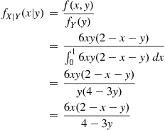
fX∣Y(x∣y)=f(x,y)fY(y)=6xy(2-x-y)∫016xy(2-x-y)dx=6xy(2-x-y)y(4-3y)=6x(2-x-y)4-3y
Hence,
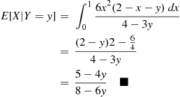
E[X∣Y=y]=∫016x2(2-x-y)dx4-3y=(2-y)2-644-3y=5-4y8-6y■
Example 3.6
The t-Distribution
If Z and Y
and Y are independent, with Z
 having a standard normal distribution and Y
 having a chi-squared distribution with n
 degrees of freedom, then the random variable T
 defined by
T=ZY/n=nZY
is said to be a t-random variable with n degrees of freedom. To compute its density function, we first derive the conditional density of T
 given that Y=y
 . Because Z
 and Y
and Y are independent, the conditional distribution of T
 given that Y=y
 is the distribution of n/yZ
 , which is normal with mean 0
 and variance n/y
 . Hence, the conditional density function of T
 given that Y=y
 is
is
fT∣Y(t∣y)=12πn/ye-t2y/2n=y1/22πne-t2y/2n,-∞<t<∞
Using the preceding, along with the following formula for the chi-squared density derived in Exercise 87 of Chapter 2,
fY(y)=e-y/2yn/2-12n/2Γ(n/2),y>0
we obtain the density function of T :
:
fT(t)=∫0∞fT,Y(t,y)dy=∫0∞fT∣Y(t∣y)fY(y)dy
With
K=1πn2(n+1)/2Γ(n/2),c=t2+n2n=121+t2n
this yields
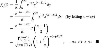
fT(t)=1K∫0∞e-cyy(n-1)/2dy=c-(n+1)/2K∫0∞e-xx(n-1)/2dx(by lettingx=cy)=c-(n+1)/2KΓn+12=Γ(n+12)πnΓ(n2)1+t2n-(n+1)/2,-∞<t<∞■
Example 3.7
The joint density of X and Y
and Y is given by
f(x,y)=12ye-xy,0<x<∞,0<y<20,otherwise
What is E[eX/2∣Y=1] ?
?
Solution: The conditional density of X , given that Y=1
 , is given by
fX∣Y(x∣1)=f(x,1)fY(1)=12e-x∫0∞12e-xdx=e-x
Hence, by Proposition 2.1,
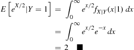
EeX/2∣Y=1=∫0∞ex/2fX∣Y(x∣1)dx=∫0∞ex/2e-xdx=2■
Example 3.8
Let X1 and X2
 be independent exponential random variables with rates μ1
 and μ2
 . Find the conditional density of X1
 given that X1+X2=t
 .
.
Solution: To begin, let us first note that if f(x,y) is the joint density of X,Y
 , then the joint density of X
 and X+Y
 is
is
fX,X+Y(x,t)=f(x,t-x)
which is easily seen by noting that the Jacobian of the transformation
g1(x,y)=x,g2(x,y)=x+y
is equal to 1 .
.
Applying the preceding to our example yields
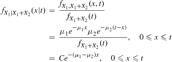
fX1∣X1+X2(x∣t)=fX1,X1+X2(x,t)fX1+X2(t)=μ1e-μ1xμ2e-μ2(t-x)fX1+X2(t),0⩽x⩽t=Ce-(μ1-μ2)x,0⩽x⩽t
where
C=μ1μ2e-μ2tfX1+X2(t)
Now, if μ1=μ2 , then
fX1∣X1+X2(x∣t)=C,0⩽x⩽t
yielding that C=1/t and that X1
 given X1+X2=t
 is uniformly distributed on (0,t)
 . On the other hand, if μ1≠μ2
 , then we use
1=∫0tfX1∣X1+X2(x∣t)dx=Cμ1-μ21-e-(μ1-μ2)t
to obtain
C=μ1-μ21-e-(μ1-μ2)t
thus yielding the result:
fX1∣X1+X2(x∣t)=(μ1-μ2)e-(μ1-μ2)x1-e-(μ1-μ2)t
An interesting byproduct of our analysis is that
fX1+X2(t)=μ1μ2e-μ2tC=μ2te-μt,ifμ1=μ2=μμ1μ2(e-μ2t-e-μ1t)μ1-μ2,ifμ1≠μ2■
3.4 Computing Expectations by Conditioning
Let us denote by E[X∣Y] that function of the random variable Y
 whose value at Y=y
 is E[X∣Y=y]
 . Note that E[X∣Y]
 is itself a random variable. An extremely important property of conditional expectation is that for all random variables X
 and Y
and Y
E[X]=EE[X∣Y] (3.2)
 (3.2)
(3.2)If Y is a discrete random variable, then Equation (3.2) states that
E[X]=∑yE[X∣Y=y]P{Y=y} (3.2a)
 (3.2a)
while if Y is continuous with density fY(y)
 , then Equation (3.2) says that
E[X]=∫-∞∞E[X∣Y=y]fY(y)dy (3.2b)
 (3.2b)
We now give a proof of Equation (3.2) in the case where X and Y
and Y are both discrete random variables.
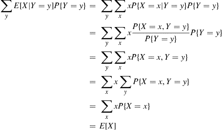
Proof of Equation (3.2) When X and Y Are Discrete. We must show that
E[X]=∑yE[X∣Y=y]P{Y=y} (3.3)
 (3.3)
(3.3)
Now, the right side of the preceding can be written
∑yE[X∣Y=y]P{Y=y}=∑y∑xxP{X=x∣Y=y}P{Y=y}=∑y∑xxP{X=x,Y=y}P{Y=y}P{Y=y}=∑y∑xxP{X=x,Y=y}=∑xx∑yP{X=x,Y=y}=∑xxP{X=x}=E[X]
and the result is obtained. ■
One way to understand Equation (3.3) is to interpret it as follows. It states that to calculate E[X] we may take a weighted average of the conditional expected value of X
 given that Y=y
 , each of the terms E[X∣Y=y]
 being weighted by the probability of the event on which it is conditioned.
The following examples will indicate the usefulness of Equation (3.2).
Example 3.9
Sam will read either one chapter of his probability book or one chapter of his history book. If the number of misprints in a chapter of his probability book is Poisson distributed with mean 2 and if the number of misprints in his history chapter is Poisson distributed with mean 5, then assuming Sam is equally likely to choose either book, what is the expected number of misprints that Sam will come across?
Solution: Letting X denote the number of misprints and letting
Y=1,if Sam chooses his history book2,if Sam chooses his probability book
then
E[X]=E[X∣Y=1]P{Y=1}+E[X∣Y=2]P{Y=2}=512+212=72■
Example 3.10
The Expectation of the Sum of a Random Number of Random Variables
Suppose that the expected number of accidents per week at an industrial plant is four. Suppose also that the numbers of workers injured in each accident are independent random variables with a common mean of 2. Assume also that the number of workers injured in each accident is independent of the number of accidents that occur. What is the expected number of injuries during a week?
Solution: Letting N denote the number of accidents and Xi
 the number injured in the i
 th accident, i=1,2,…
 , then the total number of injuries can be expressed as ∑i=1NXi
 . Now,
E∑1NXi=EE∑1NXi∣N
But
E∑1NXi∣N=n=E∑1nXi∣N=n=E∑1nXiby the independence ofXiandN=nE[X]
which yields
E∑i=1NXi∣N=NE[X]
and thus
E∑i=1NXi=ENE[X]=E[N]E[X]
Therefore, in our example, the expected number of injuries during a week equals 4×2=8 . ■
. ■
The random variable ∑i=1NXi , equal to the sum of a random number N
 of independent and identically distributed random variables that are also independent of N
 , is called a compound random variable. As just shown in Example 3.10, the expected value of a compound random variable is E[X]E[N]
 . Its variance will be derived in Example 3.19.
Example 3.11
The Mean of a Geometric Distribution
A coin, having probability p of coming up heads, is to be successively flipped until the first head appears. What is the expected number of flips required?
Solution: Let N be the number of flips required, and let
Y=1,if the first flip results in a head0,if the first flip results in a tail
Now,
E[N]=E[N∣Y=1]P{Y=1}+E[N∣Y=0]P{Y=0}=pE[N∣Y=1]+(1-p)E[N∣Y=0] (3.4)
 (3.4)
(3.4)
However,
E[N∣Y=1]=1,E[N∣Y=0]=1+E[N] (3.5)
 (3.5)
(3.5)
To see why Equation (3.5) is true, consider E[N∣Y=1] . Since Y=1
 , we know that the first flip resulted in heads and so, clearly, the expected number of flips required is 1. On the other hand if Y=0
 , then the first flip resulted in tails. However, since the successive flips are assumed independent, it follows that, after the first tail, the expected additional number of flips until the first head is just E[N]
 . Hence E[N∣Y=0]=1+E[N]
 . Substituting Equation (3.5) into Equation (3.4) yields
E[N]=p+(1-p)(1+E[N])
or
E[N]=1/p■
Because the random variable N is a geometric random variable with probability mass function p(n)=p(1-p)n-1
 , its expectation could easily have been computed from E[N]=∑1∞np(n)
 without recourse to conditional expectation. However, if you attempt to obtain the solution to our next example without using conditional expectation, you will quickly learn what a useful technique “conditioning” can be.
Example 3.12
A miner is trapped in a mine containing three doors. The first door leads to a tunnel that takes him to safety after two hours of travel. The second door leads to a tunnel that returns him to the mine after three hours of travel. The third door leads to a tunnel that returns him to his mine after five hours. Assuming that the miner is at all times equally likely to choose any one of the doors, what is the expected length of time until the miner reaches safety?
Solution: Let X denote the time until the miner reaches safety, and let Y
 denote the door he initially chooses. Now,
E[X]=E[X∣Y=1]P{Y=1}+E[X∣Y=2]P{Y=2}+E[X∣Y=3]P{Y=3}=13E[X∣Y=1]+E[X∣Y=2]+E[X∣Y=3]
However,
E[X∣Y=1]=2,E[X∣Y=2]=3+E[X],E[X∣Y=3]=5+E[X], (3.6)
 (3.6)
(3.6)
To understand why this is correct consider, for instance, E[X∣Y=2] , and reason as follows. If the miner chooses the second door, then he spends three hours in the tunnel and then returns to the mine. But once he returns to the mine the problem is as before, and hence his expected additional time until safety is just E[X]
 . Hence E[X∣Y=2]=3+E[X]
 . The argument behind the other equalities in Equation (3.6) is similar. Hence,
E[X]=132+3+E[X]+5+E[X]orE[X]=10■
Example 3.13
Multinomial Covariances
Consider n independent trials, each of which results in one of the outcomes 1,…,r
 , with respective probabilities p1,…,pr,
 ∑i=1rpi=1
 . If we let Ni
 denote the number of trials that result in outcome i
 , then (N1,…,Nr)
 is said to have a multinomial distribution. For i≠j
 , let us compute
Cov(Ni,Nj)=E[NiNj]-E[Ni]E[Nj]
Because each trial independently results in outcome i with probability pi
 , it follows that Ni
 is binomial with parameters (n,pi)
 , giving that E[Ni]E[Nj]=n2pipj
 . To compute E[NiNj]
 , condition on Ni
 to obtain
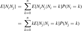
E[NiNj]=∑k=0nE[NiNj∣Ni=k]P(Ni=k)=∑k=0nkE[Nj∣Ni=k]P(Nj=k)
Now, given that k of the n
 trials result in outcome i
 , each of the other n-k
 trials independently results in outcome j
 with probability
P(j∣noti)=pj1-pi
thus showing that the conditional distribution of Nj , given that Ni=k
 , is binomial with parameters (n-k,pj1-pi)
 . Using this yields
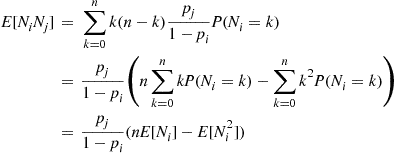
E[NiNj]=∑k=0nk(n-k)pj1-piP(Ni=k)=pj1-pin∑k=0nkP(Ni=k)-∑k=0nk2P(Ni=k)=pj1-pi(nE[Ni]-E[Ni2])
Because Ni is binomial with parameters (n,pi)
E[Ni2]=Var(Ni)+(E[Ni])2=npi(1-pi)+(npi)2
Hence,
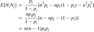
E[NiNj]=pj1-pi[n2pi-npi(1-pi)-n2pi2]=npipj1-pi[n-npi-(1-pi)]=n(n-1)pipj
which yields the result
Cov(Ni,Nj)=n(n-1)pipj-n2pipj=-npipj■
Example 3.14
The Matching Rounds Problem
Suppose in Example 2.31 that those choosing their own hats depart, while the others (those without a match) put their selected hats in the center of the room, mix them up, and then reselect. Also, suppose that this process continues until each individual has his own hat.
Solution: (a) It follows from the results of Example 2.31 that no matter how many people remain there will, on average, be one match per round. Hence, one might suggest that E[Rn]=n . This turns out to be true, and an induction proof will now be given. Because it is obvious that E[R1]=1
 , assume that E[Rk]=k
 for k=1,…,n-1
 . To compute E[Rn]
 , start by conditioning on Xn
 , the number of matches that occur in the first round. This gives
E[Rn]=∑i=0nE[Rn∣Xn=i]P{Xn=i}
Now, given a total of i matches in the initial round, the number of rounds needed will equal 1 plus the number of rounds that are required when n-i
 persons are to be matched with their hats. Therefore,
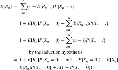
E[Rn]=∑i=0n(1+E[Rn-i])P{Xn=i}=1+E[Rn]P{Xn=0}+∑i=1nE[Rn-i]P{Xn=i}=1+E[Rn]P{Xn=0}+∑i=1n(n-i)P{Xn=i}by the induction hypothesis=1+E[Rn]P{Xn=0}+n(1-P{Xn=0})-E[Xn]=E[Rn]P{Xn=0}+n(1-P{Xn=0})
where the final equality used the result, established in Example 2.31, that E[Xn]=1 . Since the preceding equation implies that E[Rn]=n
 , the result is proven. (b) For n⩾2
 , conditioning on Xn
 , the number of matches in round 1, gives
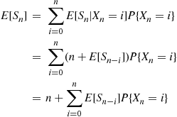
E[Sn]=∑i=0nE[Sn∣Xn=i]P{Xn=i}=∑i=0n(n+E[Sn-i])P{Xn=i}=n+∑i=0nE[Sn-i]P{Xn=i}
where E[S0]=0 . To solve the preceding equation, rewrite it as
E[Sn]=n+E[Sn-Xn]
Now, if there were exactly one match in each round, then it would take a total of 1+2+⋯+n=n(n+1)/2
 selections. Thus, let us try a solution of the form E[Sn]=an+bn2
 . For the preceding equation to be satisfied by a solution of this type, for n⩾2
 , we need
an+bn2=n+Ea(n-Xn)+b(n-Xn)2
or, equivalently,
an+bn2=n+a(n-E[Xn])+bn2-2nE[Xn]+EXn2
Now, using the results of Example 2.31 and Exercise 72 of Chapter 2 that E[Xn]=Var(Xn)=1 , the preceding will be satisfied if
an+bn2=n+an-a+bn2-2nb+2b
and this will be valid provided that b=1/2,a=1 . That is,
E[Sn]=n+n2/2
satisfies the recursive equation for E[Sn] .
.
The formal proof that E[Sn]=n+n2/2,n⩾2 , is obtained by induction on n
 . It is true when n=2
 (since, in this case, the number of selections is twice the number of rounds and the number of rounds is a geometric random variable with parameter p=1/2
 ). Now, the recursion gives
E[Sn]=n+E[Sn]P{Xn=0}+∑i=1nE[Sn-i]P{Xn=i}
Hence, upon assuming that E[S0]=E[S1]=0,E[Sk]=k+k2/2 , for k=2,…,n-1
 and using that P{Xn=n-1}=0
 , we see that
E[Sn]=n+E[Sn]P{Xn=0}+∑i=1n[n-i+(n-i)2/2]P{Xn=i}=n+E[Sn]P{Xn=0}+(n+n2/2)(1-P{Xn=0})-(n+1)E[Xn]+E[Xn2]/2

 and
and  , the conditional probability of
  given
given  is defined, as long as
  , by
, by
 and
and  are discrete random variables, then it is natural to define the conditional probability mass function of
  given that
  , by
, by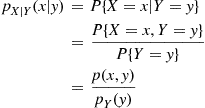
 such that
  . Similarly, the conditional probability distribution function of
  given that
  is defined, for all
  such that
  , by
, by
 given that
  is defined by
 . If
. If  is independent of
  , then the conditional mass function, distribution, and expectation are the same as the unconditional ones. This follows, since if
  is independent of
  , then

 and
and  have a joint probability density function
  , then the conditional probability density function of
  , given that
  , is defined for all values of
  such that
  , by
, by
 and the right side by
  to get
 and
and  ,
,  is approximately the conditional probability that
  is between
  and
and  given that
  is between
  and
and  .
. , given that
  , is defined for all values of
  such that
  , by
, by
 that function of the random variable
  whose value at
  is
is  . Note that
  is itself a random variable. An extremely important property of conditional expectation is that for all random variables
  and
and 
 (3.2)
(3.2) is a discrete random variable, then Equation (3.2) states that
 (3.2a)
 is continuous with density
  , then Equation (3.2) says that
 (3.2b)
 and
and  are both discrete random variables.
 (3.3)
(3.3)
 we may take a weighted average of the conditional expected value of
  given that
  , each of the terms
  being weighted by the probability of the event on which it is conditioned.
 , equal to the sum of a random number
  of independent and identically distributed random variables that are also independent of
  , is called a compound random variable. As just shown in Example 3.10, the expected value of a compound random variable is
  . Its variance will be derived in Example 3.19.
 is a geometric random variable with probability mass function
  , its expectation could easily have been computed from
  without recourse to conditional expectation. However, if you attempt to obtain the solution to our next example without using conditional expectation, you will quickly learn what a useful technique “conditioning” can be.


