
Method 2 Conditional Distribution of the Arrival Times
Recall the result for a Poisson process having rate  that given the number of events by time
  the set of event times are independent and identically distributed uniform
  random variables. Now suppose that each of these events is independently counted with a probability that is equal to
  when the event occurred at time
  . Hence, given the number of counted events, it follows that the set of times of these counted events are independent with a common distribution given by
  , where
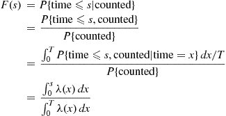
The preceding (somewhat heuristic) argument thus shows that given  events of a nonhomogeneous Poisson process by time
  the
the  event times are independent with a common density function
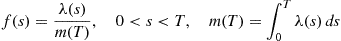 (11.10)
Since  , the number of events by time
  , is Poisson distributed with mean
  , we can simulate the nonhomogeneous Poisson process by first simulating
  and then simulating
  random variables from the density function of (11.10).
Example 11.12
If  , then we can simulate the first
  time units of the nonhomogeneous Poisson process by first simulating
  , a Poisson random variable having mean
 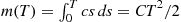 , and then simulating
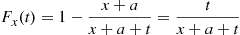
  random variables having distribution
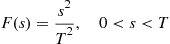
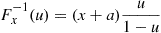
Random variables having the preceding distribution either can be simulated by use of the inverse transform method (since  ) or by noting that
  is the distribution function of
  when
when  and
and  are independent random numbers. ■
If the distribution function specified by Equation (11.10) is not easily invertible, we can always simulate from (11.10) by using the rejection method where we either accept or reject simulated values of uniform  random variables. That is, let
  . Then
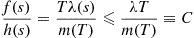
where  is a bound on
  . Hence, the rejection method is to generate random numbers
  and
and  then accept
  if
if
or, equivalently, if

Method 3 Simulating the Event Times
The third method we shall present for simulating a nonhomogeneous Poisson process having intensity function  is probably the most basic approach—namely, to simulate the successive event times. So let
  denote the event times of such a process. As these random variables are dependent we will use the conditional distribution approach to simulation. Hence, we need the conditional distribution of
  given
given  .
.
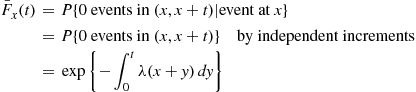
To start, note that if an event occurs at time  then, independent of what has occurred prior to
  , the time until the next event has the distribution
  given by
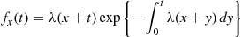
Differentiation yields that the density corresponding to  is
is
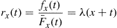
implying that the hazard rate function of  is
is
We can now simulate the event times  by simulating
  from
from  ; then if the simulated value of
  is
is  , simulate
  by adding
  to a value generated from
  , and if this sum is
  simulate
  by adding
  to a value generated from
  , and so on. The method used to simulate from these distributions should depend, of course, on the form of these distributions. However, it is interesting to note that if we let
  be such that
  and use the hazard rate method to simulate, then we end up with the approach of Method 1 (we leave the verification of this fact as an exercise). Sometimes, however, the distributions
  can be easily inverted and so the inverse transform method can be applied.
Example 11.13
Suppose that  . Then
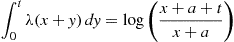
Hence,
and so
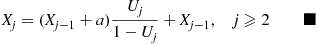
We can, therefore, simulate the successive event times  by generating
  and then setting
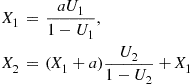
and, in general,
11.5.2 Simulating a Two-Dimensional Poisson Process
A point process consisting of randomly occurring points in the plane is said to be a two-dimensional Poisson process having rate  if
if
(a) the number of points in any given region of area  is Poisson distributed with mean
  ; and
; and
(b) the numbers of points in disjoint regions are independent.
For a given fixed point O in the plane, we now show how to simulate events occurring according to a two-dimensional Poisson process with rate  in a circular region of radius
  centered about
  . Let
. Let  , denote the distance between
  and its
  th nearest Poisson point, and let
  denote the circle of radius
  centered at
  . Then
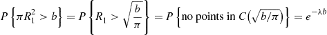
Also, with  denoting the region between
  and
and  :
:
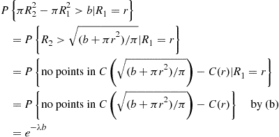
In fact, the same argument can be repeated to obtain the following.
Proposition 11.6
With  ,
,
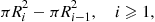
are independent exponentials with rate  .
.
In other words, the amount of area that needs to be traversed to encompass a Poisson point is exponential with rate  . Since, by symmetry, the respective angles of the Poisson points are independent and uniformly distributed over
  , we thus have the following algorithm for simulating the Poisson process over a circular region of radius
  about
about  :
:
Step 1 Generate independent exponentials with rate 1,  , stopping at

Step 2 If  , stop. There are no points in
  . Otherwise, for
 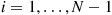 , set
, set
Step 3 Generate independent uniform  random variables
  .
.
Step 4 Return the  Poisson points in
  whose polar coordinates are

The preceding algorithm requires, on average,  exponentials and an equal number of uniform random numbers. Another approach to simulating points in
  is to first simulate
  , the number of such points, and then use the fact that, given
  , the points are uniformly distributed in
  . This latter procedure requires the simulation of
  , a Poisson random variable with mean
  ; we must then simulate
  uniform points on
  , by simulating
  from the distribution
  (see Exercise 25) and
  from uniform
  and must then sort these
  uniform values in increasing order of
  . The main advantage of the first procedure is that it eliminates the need to sort.
The preceding algorithm can be thought of as the fanning out of a circle centered at  with a radius that expands continuously from 0 to
  . The successive radii at which Poisson points are encountered is simulated by noting that the additional area necessary to encompass a Poisson point is always, independent of the past, exponential with rate
  . This technique can be used to simulate the process over noncircular regions. For instance, consider a nonnegative function
  , and suppose we are interested in simulating the Poisson process in the region between the
  -axis and
  with
with  going from 0 to
  (see Figure 11.4). To do so we can start at the left-hand end and fan vertically to the right by considering the successive areas
  . Now if
  denote the successive projections of the Poisson points on the
  -axis, then analogous to Proposition 11.6, it will follow that (with
  )
)  , will be independent exponentials with rate 1. Hence, we should simulate
  , independent exponentials with rate 1, stopping at
and determine  by
by
If we now simulate  —independent uniform
  random numbers—then as the projection on the
  -axis of the Poisson point whose
  -coordinate is
  is uniform on (0,
  ), it follows that the simulated Poisson points in the interval are
  .
.

Of course, the preceding technique is most useful when  is regular enough so that the foregoing equations can be solved for the
  . For instance, if
  (and so the region of interest is a rectangle), then

and the Poisson points are

11.6 Variance Reduction Techniques
Let  have a given joint distribution, and suppose we are interested in computing

where  is some specified function. It is often the case that it is not possible to analytically compute the preceding, and when such is the case we can attempt to use simulation to estimate
  . This is done as follows: Generate
  having the same joint distribution as
  and set
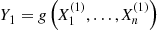
Now, simulate a second set of random variables (independent of the first set)  having the distribution of
  and set
Continue this until you have generated  (some predetermined number) sets, and so have also computed
  . Now,
  are independent and identically distributed random variables each having the same distribution of
  . Thus, if we let
  denote the average of these
  random variables—that is,

then
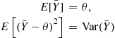
Hence, we can use  as an estimate of
  . As the expected square of the difference between
  and
and  is equal to the variance of
  , we would like this quantity to be as small as possible. In the preceding situation,
  , which is usually not known in advance but must be estimated from the generated values
  . We now present three general techniques for reducing the variance of our estimator.
11.6.1 Use of Antithetic Variables
In the preceding situation, suppose that we have generated  and
and  , identically distributed random variables having mean
  . Now,
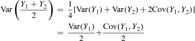
Hence, it would be advantageous (in the sense that the variance would be reduced) if  and
and  rather than being independent were negatively correlated. To see how we could arrange this, let us suppose that the random variables
  are independent and, in addition, that each is simulated via the inverse transform technique. That is,
  is simulated from
  where
where  is a random number and
  is the distribution of
  . Hence,
  can be expressed as

Now, since  is also uniform over
  whenever
  is a random number (and is negatively correlated with
  ) it follows that
  defined by

will have the same distribution as  . Hence, if
  and
and  were negatively correlated, then generating
  by this means would lead to a smaller variance than if it were generated by a new set of random numbers. (In addition, there is a computational savings since rather than having to generate
  additional random numbers, we need only subtract each of the previous
  from 1.) The following theorem will be the key to showing that this technique—known as the use of antithetic variables—will lead to a reduction in variance whenever
  is a monotone function.
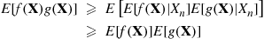
Theorem 11.1
If  are independent, then, for any increasing functions
  and
and  of
of  variables,
 (11.11)
where  .
.
Proof
The proof is by induction on  . To prove it when
  , let
, let  and
and  be increasing functions of a single variable. Then, for any
  and
and  ,
,

since if  then both factors are nonnegative (nonpositive). Hence, for any random variables
  and
and  ,
,

implying that

or, equivalently,

If we suppose that  and
and  are independent and identically distributed, as in this case, then

and so we obtain the result when  .
.
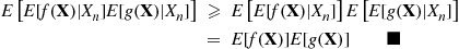
So assume that (11.11) holds for  variables, and now suppose that
  are independent and
  and
and  are increasing functions. Then

Hence,

and, upon taking expectations of both sides,
The last inequality follows because  and
and  are both increasing functions of
  , and so, by the result for
  ,
,
Corollary 11.7
If  are independent, and
  is either an increasing or decreasing function, then

Proof
Suppose  is increasing. As
  is increasing in
  , then, from Theorem 11.1,

When  is decreasing just replace
  by its negative. ■
Since  is increasing in
  (as
(as  , being a distribution function, is increasing) it follows that
  is a monotone function of
  whenever
  is monotone. Hence, if
  is monotone the antithetic variable approach of twice using each set of random numbers
  by first computing
  and then
  will reduce the variance of the estimate of
  . That is, rather than generating
  sets of
  random numbers, we should generate
  sets and use each set twice.
Example 11.14
Simulating the Reliability Function
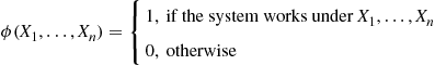
Consider a system of  components in which component
  , independently of other components, works with probability
  . Letting
suppose there is a monotone structure function  such that
We are interested in using simulation to estimate

Now, we can simulate the  by generating uniform random numbers
  and then setting

Hence, we see that

where  is a decreasing function of
  . Hence,

and so the antithetic variable approach of using  to generate both
  and
and  results in a smaller variance than if an independent set of random numbers was used to generate the second
  . ■
. ■
Example 11.15
Simulating a Queueing System
Consider a given queueing system, let  denote the delay in queue of the
  th arriving customer, and suppose we are interested in simulating the system so as to estimate

Let  denote the first
  interarrival times and
  the first
  service times of this system, and suppose these random variables are all independent. Now in most systems
  will be a function of
  —say,
—say,

Also,  will usually be increasing in
  and decreasing in
  . If we use the inverse transform method to simulate
  —say,
—say,  where
where  are independent uniform random numbers—then we may write

where  is increasing in its variates. Hence, the antithetic variable approach will reduce the variance of the estimator of
  . (Thus, we would generate
  and set
  and
and  for the first run, and
  and
and  for the second.) As all the
  and
and  are independent, however, this is equivalent to setting
  in the first run and using
  for
for  and
and  for
for  in the second. ■
11.6.2 Variance Reduction by Conditioning
Let us start by recalling (see Proposition 3.1) the conditional variance formula
 (11.12)
Now suppose we are interested in estimating  by simulating
  and then computing
  . Now, if for some random variable
  we can compute
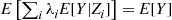
  then, as
  , it follows from the conditional variance formula that

implying, since  , that
  is a better estimator of
  than is
  .
.
In many situations, there are a variety of  that can be conditioned on to obtain an improved estimator. Each of these estimators
  will have mean
  and smaller variance than does the raw estimator
  . We now show that for any choice of weights
  is also an improvement over
  .
.

Proof
The proof of (a) is immediate. To prove (b), let  denote an integer valued random variable independent of all the other random variables under consideration and such that

Applying the conditional variance formula twice yields

Example 11.16
Consider a queueing system having Poisson arrivals and suppose that any customer arriving when there are already  others in the system is lost. Suppose that we are interested in using simulation to estimate the expected number of lost customers by time
  . The raw simulation approach would be to simulate the system up to time
  and determine
  , the number of lost customers for that run. A better estimate, however, can be obtained by conditioning on the total time in
  that the system is at capacity. Indeed, if we let
  denote the time in
  that there are
  in the system, then

where  is the Poisson arrival rate. Hence, a better estimate for
  than the average value of
  over all simulation runs can be obtained by multiplying the average value of
  per simulation run by
  . If the arrival process were a nonhomogeneous Poisson process, then we could improve over the raw estimator
  by keeping track of those time periods for which the system is at capacity. If we let
  denote the time intervals in
  in which there are
  in the system, then
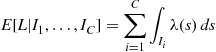
where  is the intensity function of the nonhomogeneous Poisson arrival process. The use of the right side of the preceding would thus lead to a better estimate of
  than the raw estimator
  . ■
. ■
Example 11.17
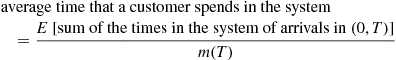
Suppose that we wanted to estimate the expected sum of the times in the system of the first  customers in a queueing system. That is, if
  is the time that the
  th customer spends in the system, then we are interested in estimating

Let  denote the “state of the system” at the moment at which the
  th customer arrives. It can be shown§ that for a wide class of models the estimator
  has (the same mean and) a smaller variance than the estimator
  . (It should be noted that whereas it is immediate that
  has smaller variance than
  , because of the covariance terms involved it is not immediately apparent that
  has smaller variance than
  .) For instance, in the model
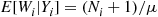
where  is the number in the system encountered by the
  th arrival and
  is the mean service time; the result implies that
 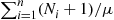 is a better estimate of the expected total time in the system of the first
  customers than is the raw estimator
  . ■
. ■
Example 11.18
Estimating the Renewal Function by Simulation
Consider a queueing model in which customers arrive daily in accordance with a renewal process having interarrival distribution  . However, suppose that at some fixed time
  , for instance 5 P.M., no additional arrivals are permitted and those customers that are still in the system are serviced. At the start of the next and each succeeding day customers again begin to arrive in accordance with the renewal process. Suppose we are interested in determining the average time that a customer spends in the system. Upon using the theory of renewal reward processes (with a cycle starting every
  time units), it can be shown that
where  is the expected number of renewals in (0,
  ).
).
If we were to use simulation to estimate the preceding quantity, a run would consist of simulating a single day, and as part of a simulation run, we would observe the quantity  , the number of arrivals by time
  . Since
  , the natural simulation estimator of
  would be the average (over all simulated days) value of
  obtained. However, Var
 is, for large
  , proportional to
  (its asymptotic form being
  , where
  is the variance and
  the mean of the interarrival distribution
  ), and so, for large
  , the variance of our estimator would be large. A considerable improvement can be obtained by using the analytic formula (see Section 7.3)
 (11.13)
where  denotes the time from
  until the next renewal—that is, it is the excess life at
  . Since the variance of
  does not grow with
  (indeed, it converges to a finite value provided the moments of
  are finite), it follows that for
  large, we would do much better by using the simulation to estimate
  and then using Equation (11.13) to estimate
  .
.
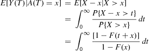
However, by employing conditioning, we can improve further on our estimate of  . To do so, let
  denote the age of the renewal process at time
  —that is, it is the time at
  since the last renewal. Then, rather than using the value of
  , we can reduce the variance by considering
  . Now, knowing that the age at
  is equal to
  is equivalent to knowing that there was a renewal at time
  and the next interarrival time
  is greater than
  . Since the excess at
  will equal
  (see Figure 11.5), it follows that
which can be numerically evaluated if necessary.
As an illustration of the preceding note that if the renewal process is a Poisson process with rate  , then the raw simulation estimator
  will have variance
  ; since
  will be exponential with rate
  , the estimator based on (11.13) will have variance
  . On the other hand, since
  will be independent of
  (and
(and  ), it follows that the variance of the improved estimator
  is 0. That is, conditioning on the age at time
  yields, in this case, the exact answer. ■
Example 11.19
Consider the  queueing system where customers arrive in accordance with a Poisson process with rate
  to a single server having service distribution
  with mean
  . Suppose that, for a specified time
  , the server will take a break at the first time
  at which the system is empty. That is, if
  is the number of customers in the system at time
  , then the server will take a break at time

To efficiently use simulation to estimate  , generate the system to time
  ; let
; let  denote the remaining service time of the customer in service at time
  , and let
  equal the number of customers waiting in queue at time
  . (Note that
  is equal to
  if
if  , and
, and  .) Now, with
  equal to the number of customers that arrive in the remaining service time
  , it follows that if
  and
and  , then the additional amount of time from
  until the server can take a break is equal to the amount of time that it takes until the system, starting with
  customers, becomes empty. Because this is equal to the sum of
  busy periods, it follows from Section 8.5.3 that
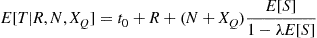
Consequently,

Thus, rather than using the generated value of  as the estimator from a simulation run, it is better to stop the simulation at time
  and use the estimator
  . ■
. ■


11.6.3 Control Variates
Again suppose we want to use simulation to estimate  where
where  . But now suppose that for some function
  the expected value of
  is known—say,
  . Then for any constant
  we can also use

as an estimator of  . Now,