INTRODUCTION
This chapter uses neoclassical and classical economic growth models to explain patterns of productivity under the commune (1958–1983). It reveals how China revived agricultural production after the Great Leap Forward (GLF) famine and lackluster productivity in the 1960s and generated sizable increases in food output in the 1970s. High rates of income extraction from households (i.e., forced savings), productive investment, and technological progress drove increased food output under the commune. This process was akin to the “transformation in techniques” that E. L. Jones argued English agriculture experienced before that country’s industrial revolution.1 As detailed in chapter 3, between 1970 and 1979, higher savings rates underwrote investments in more and better agricultural capital and technologies (see chapter 3, figures 3.6–3.20) that increased agricultural production (see chapter 1, figures 1.1–1.3).
The key question for a developing country with an extremely large or fast-growing population is how to increase savings rates and make productive investments that take advantage of high returns to capital. The commune extracted an increasing percentage of household savings to finance productive capital and technology, thus kick-starting a continuous development process that produced rapid growth in food production. Through the extraction of household savings, Chinese communes funded investments that increased agricultural productivity. The workpoint remuneration system constituted a “kabuki theater” that used a multitude of meetings about job allocations, work evaluations, and workpoints to attract members’ attention toward the size of their portion relative to others and away from the system’s extraction of their savings. The agricultural research and extension system, which was covered in chapter 3, targeted investments into land and labor-saving capital improvements and technical innovations and rewarded locally appropriate, results-driven investments. Meanwhile, the formal recognition of household—the basic accounting unit before 1958 and again after decollectivization—private plots, cottage industries, and rural markets (i.e., the Three Small Freedoms) ensured at least a minimum consumption floor to prevent the return of famine.
I use a neoclassical economic growth model (i.e., the Solow–Swan model) to identify six distinct phases of savings and investment during China’s collective agriculture era:
1. Pre-commune: undersaving
2. GLF Commune (1958–1961): oversaving with unproductive investment and high capital depreciation rates
3. The Rightist Commune (1962–1964): return to undersaving
4. The Leftist Commune (1965–1969): high savings rates but without increases in investment productivity
5. The Green Revolution Commune (1970–1979): high savings rates with increases in productive investment
6. Decollectivization (1980–1983): a return to undersaving
Phases 2–5 correspond with the four phases of commune development examined in chapters 2 and 3. This analysis reveals, among other things, how decollectivization delivered a consumption boost to impoverished rural households.
This chapter has two sections. The first section uses the Solow–Swan neoclassical economic growth model and the Lewis modified classical model to explain how a country like commune-era China—that is, a closed economy with an essentially unlimited and fast-growing labor supply, scarce land, quickly depreciating capital, and rising savings rates—could have generated sustained increases in agricultural output. These theories of economic growth clarify how changes in per capita rates of savings (s), consumption (c), population growth (n), capital (k), and relative capital productivity (α), as well as total factor productivity (A) and capital depreciation (δ), affect levels of per capita agricultural output (y).
The second section explains how the commune could increase savings rates without pushing households below minimum levels of consumption. It identifies variations in savings rates over the life of the commune and explains how household resources were extracted: the workpoint system, ad hoc equality-promoting policies, and rural credit cooperatives (RCCs). The chapter concludes with a discussion of the Three Small Freedoms and how they helped prevent a return to the overextraction that occurred under the GLF Commune.
THE TRANSITIONAL DYNAMICS OF PRODUCTIVITY GROWTH UNDER THE COMMUNE
This section applies insights from both the Solow–Swan neoclassical economic growth model and the Lewis modified classical model to explain how extracting household savings and investing them in productive capital and technology can generate long-run increases in agricultural output. These economic models identify explanatory variables—rates of savings, population growth, capital accumulation and depreciation, and technological progress—and their influence on agricultural output during the commune period. Note that when applying any theory to a complex empirical phenomenon, questions of “fit” inevitably arise. Being mindful that a perfect fit is not possible, it is important to recall that the limited aim of this exercise is to apply basic insights from the Solow–Swan model and the Lewis model to organize and explain patterns observed in the empirical data. These economic growth models provide internally consistent structures that may explain the long-run consequences of policies adopted during the commune period. They help identify causal variables that explain the trajectory of economic growth over time. With the help of my colleague at the University of Texas at Austin, economist Richard Lowery, I was able to represent these stylized displays using consistent numerical specifications.
These two models are particularly well suited for this case for two reasons. First, both assume a closed economy in which households cannot buy foreign goods or sell their goods abroad. Chinese communes were highly self-reliant and, with rare exceptions, were entirely insulated from foreign trade. In a closed economy, output equals income, and the amount invested equals the amount saved. Indeed, in 1970s China, the resources communes extracted from households (i.e., labor, grain, cash) were almost always spent or invested within the locality itself, such that savings and investment were practically identical.2 Communes lacked access to outside equity or debt markets, sustained deficit spending was impossible, and local financial institutions (e.g., the RCCs) could not lend beyond their deposits.
Second, both models assume one-sector production (i.e., agriculture) in which output is a homogeneous good that can be consumed or invested to create new units of capital. Again, this condition fits with the commune’s “grain first” mandate and its reliance on animal husbandry, especially swine. Thus, both the simple Solow–Swan neoclassical economic growth model and the Lewis modified classical model are well suited to explain why the commune was successful in increasing productivity.
The Solow–Swan Neoclassical Economic Growth Model
According to the neoclassical economic growth model, if an economy experiences increased rates of population growth and capital depreciation and responds with policies that increase the savings rate and channel resources into productive capital and technology, then returns to capital will remain relatively high and output will likely increase over a sustained period of time. To observe this, consider an aggregate production function including total factor productivity,3 which is given by:

Equation (4.1) represents total output, Y, as a function of the level of technological progress, A, capital input, K, and labor input, L. The level of technological progress is assumed in the Solow–Swan model to change at a steady rate that is exogenously given. I argue that there was an increase in the pace of technological advance attributable to institutional changes in the commune system introduced by the Communist Party in the 1970s.4 K is an aggregate index of capital goods and should be interpreted broadly to include both human and physical capital.5 L varies over time based on population growth. The Solow–Swan model assumes population growth is exogenous and occurs at a constant rate, n = ΔL/L ≥ 0. An increase in A, K, or L will lead to an increase in output. Multiplying both sides by  yields an expression in per capita terms given by:

This differential ∂k/∂t refers to the derivative of the per worker capital stock with respect to time. In steady state, k is constant so that ∂k/∂t = 0. In steady state, the levels of K, L, and C grow at the same rate as population growth, n, so that the per capita quantities k, y, and c do not grow. In figure 4.1, this point is determined by the intersection of the s * A * f(k) curve and the (n + δ) * k line. The curve reflects the increase in capital per worker from saving that is invested, whereas the line reflects the decrease in capital per worker resulting from a growing population and capital depreciation. The capital stock is constant at the point at which the curve and line intersect. Any given positive level of s and A has a steady-state equilibrium.
According to neoclassical economic theory, the savings rate, s, is determined by households through a cost–benefit analysis of the utility of consuming today versus consuming at a future time. Thus, s is the fraction of output saved and 1-s is the fraction of output consumed. The determination of s is complex; Robert Barro and Xavier Sala-i-Martin claim it is “a complicated function for which there are typically no closed-form solutions.”6 Under the commune, cadres determined the level of extraction, not the households themselves. Thus, in the current application, I assume s is given exogenously, such that 0 < s < 1.
At any point in time, a constant fraction of capital stock is exhausted and becomes unproductive so that capital depreciates at rate δ. If s were zero, k would decline because of a combination of capital depreciation at rate, δ, and growth in the labor force, L, at rate n. Because a constant proportion of output (i.e., the portion saved) is invested, we can represent the change in capital per worker as:
Equation (4.4) constitutes the Solow–Swan model’s fundamental nonlinear differential equation determining the change in capital per worker. At any time, the change in capital per worker is equal to gross investment minus the effective depreciation rate.
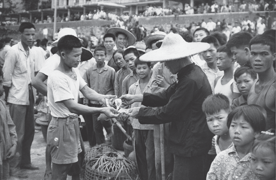
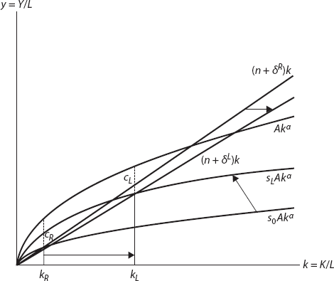
Figure 4.1 illustrates the workings of equation (4.4). The upper curve is the production function, Af(k), which determines total output. The curve for gross investment, sAf(k), reflects the share of total output that is saved, s, and invested as capital. This capital accumulation curve begins at the origin: if the capital stock is zero, then output is zero so that savings and investment are also zero. For any given level of k, gross output is given by Af(k). Gross per capita investment is equal to the height of the sAf(k) curve, and per capita consumption, represented by the dotted line, is equal to the vertical difference between the Af(k) and sAf(k) curves. Reflecting the model’s assumption of diminishing marginal returns to capital, the sAf(k) curve has a positive slope, but it flattens out as k increases. The right-hand term in equation (4.4) determines the effective rate of capital depreciation, (n +δ)k, needed to maintain a constant capital stock per worker. It appears in figure 4.1 as a straight line from the origin with positive slope n + δ. If the capital stock is zero, effective depreciation is zero. The constant slope reflects the constant rate of effective depreciation per unit of capital per worker.
Figure 4.1 represents the stated objective of the GLF Commune (1958–1961): increase savings rates, capital formulation, and capital productivity to lift per capita consumption. The impact of these actions is indicated by an increase from α to α′, which lifts the production curve, and by an increase in s0 to sGLF, which rotates the savings function upward. Equilibrium k now increases from ko to kgoal. GLF planners had hoped the capital built during the GLF would be of consistent quality with previous investments; hence, the depreciation line does not rotate. Planners had intended for the level of capital accumulation to increase from ko to kgoal and for the level of consumption to rise from co to cgoal.
Figures 4.2–4.5 provide a stylized graphic representation of the five-stage transitional dynamics that I argue occurred throughout the commune era and decollectivization (1958–1983).
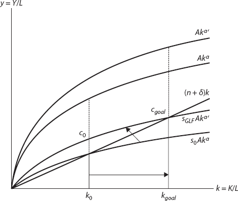
Tragically, the GLF Commune did not work as expected. Figure 4.2 captures the resulting famine. As planned, savings rates increased from s0 to sGLF, while households saw their share of total collective income (i.e., consumption) fall 13 percent—from 63.7 percent in 1956 to 50.7 percent in 1959 (figure 4.8). However, the poor quality of capital constructed and the maltreatment of skilled workers during the GLF produced a sizeable counterclockwise rotation in the constant capital stock per worker line around the axis. This caused a collapse in the capital stock, represented by the decrease from ko to kGLF. The GLF famine, represented by a sizable reduction in per capita consumption from co to cGLF, was caused by over extraction combined with poor quality investments that pushed consumption below minimum caloric levels. However, because a large portion of the 15–30 million people who perished during the GLF were either old or young—that is, not of childbearing age—population growth rate fell only briefly.7
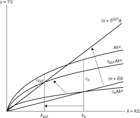
During the Rightist Commune (1962–1964; captured in figure 4.3), China, led by Liu Shaoqi and Deng Xiaoping, pursued a strategy to increase consumption to alleviate the famine. To guarantee a consumption floor for households, the government introduced contract farming, household-administered private plots, and cottage industries and expanded free markets. By 1961, households had returned to consuming more than 60 percent of total collective income, and between 1962 and 1965, household consumption remained relatively high, averaging 57.3 percent (figure 4.8.) Lowering the GLF high savings rates shifted the saving function downward to its original position. The result of this strategy was an increase in per capita consumption (as indicated in figure 4.3) because cR, the vertical distance between Akα and s0Akα evaluated at kR, exceeds cGLF, the vertical distance between Akα and sGLFAkα evaluated at kGLF. This increase in consumption was made possible by a reduction in capital formation, as indicated by the fall from kGLF to kR.
Although less capital was built during this period, what was built was of better quality and depreciated less rapidly than shoddy GLF capital. Meanwhile, after the famine subsided, population growth rates rebounded (chapter 3, figure 3.3). Considered together, these effects offset each other, such that the constant capital per worker line remained unchanged. As capital per worker and output per worker fell, a collateral effect was an increase in the marginal product of capital (given by the slope of the production function). That increase had important future consequences: it meant investment became more productive, in the sense that it had a higher yield.
During the Leftist Commune (1965–1969; depicted in figure 4.4), the Maoists regained control of rural policy and increased the savings rates (figure 4.8). This policy is represented as an increase in the rate of saving from s0 to sL, which shifted the investment curve upward. The results of this increased investment included an increased rate of capital accumulation, a slower rate of capital depreciation, and a rise in both steady-state capital per worker and output per worker. During this phase, the Cultural Revolution and the overhaul of the agricultural research and extension system (described in chapter 3) initially slowed new capital formulation; however, the farm implements and simple machines that were made during the Leftist Commune period were of better quality than those made during the Rightist Commune period. Meanwhile, the population growth rate remained high, thus offsetting much (but not all) of the effect of falling capital depreciation rates. As a result, throughout this period of rapid investment (indicated by the rise in capital stock from kR to kL), we observe a transitional period of continued low consumption, culminating in a slight reduction from cR to cL.
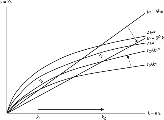
The Green Revolution Commune (1970–1979), which was initiated after policy reforms adopted at the 1970 Northern Agricultural Conference, is represented in figure 4.5. Household savings rates increased in the 1970s as represented by a return from sL to sG. By 1971, households’ share of gross collective income had dipped to 55.9 percent and it continued to fall to a low of 50.7 percent in 1976—the same rate as in 1959, the height of the GLF (figure 4.8). The primary reason for the reduction in the members’ share appears to be an increase in the percentage of collective income used for production costs (shengchan feiyong). Meanwhile, as shown in chapter 3, successful institutional changes in the workpoint remuneration system and the agricultural research and extension system contributed substantially to the expanded use of hybrid seed varieties, chemical fertilizers, mechanization, and irrigation. Figure 4.5 depicts how these institutional changes combined to increase the rate of technological innovation and improve capital productivity from a to ag, which caused both the production function and aggregate saving function to rotate counterclockwise. With capital more productive, a given saving rate now generated more productive investments. The higher quality capital built during this period, together with the nationwide introduction of birth control, produced a clockwise rotation of the constant capital per worker line around the axis. Taken together, high savings rates, more productive capital, rapid technological progress, lower depreciation rates, and reduced population growth rates had the cumulative effect of increasing the steady-state equilibrium capital stock per worker from kL to kG, while consumption per worker rose only modestly, from cL to cG. Although the transition path during this period involves spells of reduced consumption, the result is a slightly higher consumption level because the capital stock was more productive and of superior quality. Under China’s Green Revolution Commune, output per worker rose, enabling a simultaneous acceleration of capital formation along with a small increase in consumption per capita.
Decollectivization (figure 4.6), that is, the nationwide reintroduction of household-based agriculture, began in earnest with the power transition at the Fifth Plenum of the Eleventh Party Congress in February 1980 and ended in October 1983 with the “Circular on separating the local government from communes and establishing township governments” (see appendix C). During this period, savings rates fell back to approximately precommune levels, from sG to s0, thus causing the savings function, which drives capital accumulation, to shift downward. As communes were dissolved, although the depreciation and population growth rates remained constant, the pace of rural capital construction fell off considerably, which reduced the stock of per capita rural capital from kG to kD. This fall can also be observed in the amount of total investment in agriculture (chapter 3, figure 3.1), machine cultivated land (figure 3.15), irrigation systems (figure 3.14), technical and teacher training (figure 3.6), and pesticide production (figure 3.12).8 If we compare figure 4.1 with figure 4.5, it appears that between 1970 and 1979 Chinese policymakers achieved the goals promulgated during the GLF. They were able to induce higher savings rates and invest wisely in more and better agricultural capital and technologies that increased agricultural production.
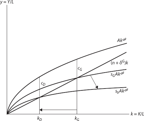
Politically, the most important aspect of this period is the transition path of increased per capita consumption from cG to cD, which consolidated the reformist faction’s political control by securing grassroots support for additional anti-Maoist reforms while also keeping as many farmers as possible in the countryside.9 Between 1980 and 1983, as the workpoint system was gradually ended, household consumption increased as a percentage of collective income from 53.1 percent to 73.9 percent (see figure 4.8). This consumption increase was accompanied by a rise in the procurement price of grain purchased from now-independent household producers, and the widespread privatization of formerly collective lands and property, which often went to former commune and brigade cadres-turned-entrepreneurs. In economic terms, the early 1980s was a transitional period during which decollectivization allowed rural localities to consume the output of the existing capital stock without reinvesting.
To summarize, the transitional dynamics of growth during the commune were as follows: Initially, excessive extraction of rural household labor and savings was coupled with large-scale investments in poor quality capital and techniques, which caused the GLF catastrophe. Reforms taken in 1962 increased consumption rates, but at the expense of capital investment. After 1970, consumption was again constrained but, unlike during the GLF and the Leftist Commune period, the funds were put toward productive investments, while sideline private plots helped prevent the overextraction of household resources. Finally, during decollectivization, household consumption returned to pre-commune levels, a change illustrated in figure 4.6 by a return from sG to s0. That boosted per capita consumption from cG to cD while reducing capital investment from kG to kD.
In the next section, I examine how China—a poor county with a large and growing population—was able to increase savings rates to fund productive investments and innovations. But first, I will show how, under the same conditions, the modified classical economic growth model yields similar predictions to the neoclassical framework.
The Lewis Modified Classical Model10
The Lewis modified classical model assumes unlimited labor supplies and can explain the sustained output growth in commune-era China. “An unlimited supply of labour,” writes Lewis, “exists in those countries where population is so large relative to capital and natural resources, that there are large sectors of the economy where the marginal productivity of labour is negligible, zero, or even negative.” Lewis observes that the assumption of unlimited labor supplies best explains “the greater part of Asia [where] labour is unlimited in supply, and economic expansion certainly cannot be taken for granted.” Under such conditions, “new industries can be created or old industries expanded without limit at the existing wage; or, to put it more exactly, shortage of labour is no limit to the creation of new sources of employment.” This is because, despite surplus labor supplies in traditional rural economies like precommune China, “the family holding is so small that if some members of the family obtained other employment the remaining members could cultivate the holding just as well.”11
According to the Lewis model, an unlimited pool of labor means that returns to capital would not diminish over time, as the Solow–Swan neoclassical model predicts would occur without technical innovation. Instead, in the classical model, returns to capital continue to grow unabated until surplus labor is used up. Lewis theorized how sustained high savings rates under conditions of unlimited labor supplies can kick-start a continuous cycle of capital accumulation:
The key to this process is the use which is made of the capitalist surplus. In so far as this is reinvested in creating more capital, the capitalist sector expands, taking more people into capitalist employment out of the subsistence sector. The surplus is then larger still, capital formation is still greater, and so the process continues until the labour surplus disappears.12
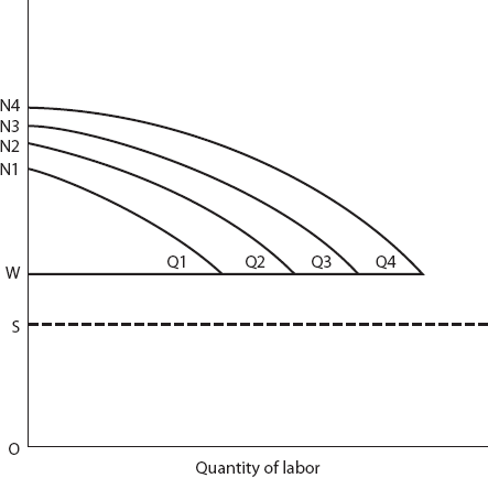
This development process is illustrated in figure 4.7, which is reproduced from Lewis’ original text. OS represents average subsistence earnings levels, and OW represents actual earnings levels after providing for additions to productive capital. The marginal productivity of labor is captured by the curves denoted NQ, with higher curves corresponding to production with a larger capital stock. The economic surplus available for investment is the area above the OW line and below the marginal productivity of labor schedule.
Because a fixed percentage of the economic surplus is reinvested, the quantity of capital increases at a constant rate, causing the marginal productivity of labor schedule to shift right from N1Q1 to N2Q2. Both the surplus and the percentage of workers earning income at OW are now larger. Further investment pushes the marginal productivity of labor to N3Q3 and then to N4Q4 and beyond, until all surplus labor is exhausted. At this stage, known as the Lewis turning point, wages start to rise above OW because of the emergence of labor scarcity.13 This simple diagrammatic framework reveals how, once started, China was able to maintain continuous and sizeable increases in agricultural output throughout the 1970s.
As with the Solow–Swan neoclassical model, the classical model considers that investments in both agriculture capital and technology are determined by savings. This savings requires refraining from consuming a portion of current output today and investing it in “capital goods which the introduction of new technology requires.”14 The big difference, however, is that the classical model assumes unlimited labor supplies at a constant real wage, which means capital per worker (k) can increase at a constant rate in perpetuity. This is because, for any quantity of K, a corresponding amount of L can be made available at the current subsistence wage rate. Income remains stable throughout the economic expansion and practically the whole profit generated by capital accumulation goes back to capital holders—or, in China’s case, the commune. Labor welfare improves because more workers benefit from being employed at a wage above subsistence. Agricultural workers may also benefit from skills training they receive during the development process and from a higher caloric intake thanks to improved food quality. In this fashion, an economy with unlimited labor and a growing capital stock can experience unlimited capital widening, while aggregate output continues to grow. This contrasts with the Solow–Swan neoclassical growth model, in which growth raises the capital-to-labor ratio, thereby raising the marginal productivity of labor and compelling capital holders to pay a higher wage.
According to Lewis, capital holders consume a portion of their profits and use the rest to support further capital formulation to generate continued returns, which, in turn, increases their capacity to make future productive investments. This means that if an agricultural revolution led by capital expansion and technical innovations were to occur in times of sustained high savings and unlimited labor supplies—as occurred in 1970s China—practically the whole surplus would become available to capital holders (i.e., the commune) for subsequent rounds of productive investment.15
The classical framework takes capital accumulation and technical progress as part of a unified development process and does not distinguish between the distinctive effects of each. Lewis argues that capital and technological progress come together with new capital embodying the latest technology. Thus, Lewis directly incorporates technical innovation into his model and stresses its importance as a source of sustained returns to capital that is inseparable from capital itself: “If we assume technical progress in agriculture, no hoarding, and unlimited labour at a constant wage, the rate of profit on capital cannot fall. On the contrary it must increase, since all the benefit of technical progress in the capitalist sector accrues to the capitalists.”16
Building on this, Nicholas Kaldor explains that technology is regularly applied in tandem with agricultural capital in ways that increase the productivity of both labor and land:
Since land is scarce, increases in production, using the same technology, are subject to diminishing returns to capital and labour, but with the passing of time, agricultural output per acre rises as a result of land-saving changes in technology (which does not exclude that many of the inventions or innovations are labour-saving as well as land-saving) and their adoption requires capital investment for their exploitation (a tractor, or a combine harvester, or even a new type of seed which promises higher yields but it more costly than previous types).17
The problem of increasing land scarcity worried David Ricardo, who observes that economic development inevitably increases the relative scarcity of land.18 According to Kaldor, in a land-scarce country with unlimited labor, unless “offset by land-saving innovations,” increasing capital investment in agriculture will cause marginal productivity of labor to decline.19 Thus, assuming that most surplus labor is employed in agriculture, the objective of technological innovation is to increase output per unit land. Agricultural economist Bruce Stone operationalizes this concept for China, arguing that “yield growth of principal staple food crops” is among “the principal criteria for judging technical change at the initial stage of modern agricultural development in a large but land-scarce peasant economy.”20 Expanding on Lewis, innovations that increase output per unit land are the only type of technological progress necessary to explain “a constant rate of growth [when] labour exists in super-abundance,” argues Kaldor.
The critical factor in continued economic growth is the persistence or continuance of land-saving innovations—man’s ability to extract more things, and a greater variety of things, from nature. Thus, in the simple model just presented, land-saving technical progress in agriculture is the only kind of technical change assumed, and this is sufficient to keep the system growing at a constant rate of growth, at least as long as growth is not hampered by the scarcity of labour—so long as labour exists in super-abundance.21
In both the neoclassical and classical models discussed previously, increased savings rates are essential to support capital accumulation. The problem for countries that have scarce capital and land but an abundant and fast-growing labor supply living near subsistence levels is how to generate the savings rates necessary to take advantage of high returns to capital. If an economy has unlimited workers living at subsistence and very little capital—as China did when the communes were created—how can it extract the resources necessary to kick-start development? Thus, “the central problem in the theory of economic development,” according to Lewis, is how an economy with an unlimited labor force living at or just above subsistence can cut consumption and save more. “People save more because they have more to save,” he concludes. “We cannot explain any industrial revolution until we can explain why saving increased.”22
INVESTMENT UNDER THE COMMUNE
Increased Savings Rates
The commune’s coercive extraction of the savings of participating households funded the 1970s agricultural modernization scheme. It removed resources from total income ex ante—that is, before the remuneration of commune members. First costs—both managerial and production—were removed, next state taxes were removed, and then a portion was set aside for public services and good works. Only after the collective took its share was the remainder distributed to members based on the number of workpoints they earned that season. By taxing households before remuneration, this process disguised austerity; it reduced consumption and ensured the high savings rates necessary to finance agricultural modernization.
During team meetings, commune members were informed of relevant agricultural modernization plans—such as mechanization and infrastructural, educational, and technological improvements—and were obliged to “vote” for them. The only agricultural investments controlled by households were those on their small sideline private plots, which accounted for 5–7 percent of total agricultural lands. These household-administered private plots, which were first introduced after the GLF and reaffirmed in 1970, guaranteed a consumption floor for households by preventing the overextraction that had pushed them below subsistence levels during the GLF. Placed in terms of the neoclassical model, during the GLF (figure 4.2), overzealous policymakers extracted too much and pushed consumption below minimum caloric levels, thus causing millions to starve. By guaranteeing household control over small private plots, officials helped reassure households that overextraction would not happen again.
Over the course of three years in the mid- to late 1950s, farmers saw their share of total collective income (i.e., consumption) fall 13 percent—from 63.7 percent in 1956 to 50.7 percent in 1959.23 By 1961, households had returned to consuming more than 60 percent of total income, and between 1962 and 1965, household consumption remained relatively high, averaging 57.3 percent. Data are unavailable for the 1966–1969 period, but by 1971, the members’ share of gross income had dipped to 55.9 percent. This share continued to fall to a low of 50.7 percent in 1976, which was the same rate as in 1959 at the height of the GLF. Consumption remained low at 51.4 percent in 1977, but beginning that year (the year after Mao’s death) the percentage of income allocated to commune members rose quickly, until it peaked at 73.9 percent in 1983, the commune’s last year (figure 4.8).24
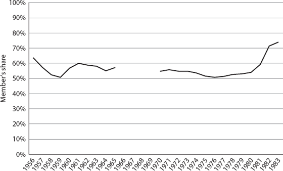
Source: Agricultural Economic Statistics 1949–1983 [Nongye jingji ziliao, 1949–1983] (Beijing: Ministry of Agriculture Planning Bureau), 515.
The primary reason for the reduction in the members’ share between 1961 and 1977 was the increase in production costs (shengchan feiyong). For a decade, between 1956 and 1965, production costs remained constant at about 25–26 percent of total income. Statistics are unavailable for 1966–1969, but they were 27.9 percent in 1970, before jumping from 27.3 percent to 30.1 percent between 1971 and 1972. Production costs continued to rise, peaking in 1978 at 32.3 percent, before falling precipitously to a nadir of 22.9 percent in 1983.25
Decollectivization, begun in earnest in 1980, marked a return not only to traditional patterns of organization (i.e., village, township, county) but also to traditional rates of rural undersaving and high consumption.26 Between 1979 and 1983, the percentage of household consumption of total collective income rose 20.8 percent—from 53.1 percent to 73.9 percent (figure 4.8). As early as January 1978, in response to “low standards of living,” farmers were again favoring “immediate consumption as against collective savings to be devoted to agricultural innovations,” observes agricultural economist Lau Siukai.
One of the most important reasons for the resistance to innovations encountered in the rural areas in China is the preference of many peasants for immediate consumption as against collective savings to be devoted to agricultural innovations in the future and this phenomenon can be readily evidenced in the controversy over agricultural mechanization within the communes. Given the low standard of living of the peasants at the present moment, it is understandable that they would opt for a higher consumption/saving ratio.27
The excessive extraction of rural household labor and savings coupled with large-scale investments in poor-quality capital and techniques caused the GLF catastrophe. Consumption was again constrained in the 1970s, but unlike during the GLF, the funds were put toward productive investments, and sideline private plots helped prevent the overextraction of household resources. During decollectivization, household consumption increased as a percentage of total income. This change is illustrated in figure 4.6 by a return from sGto s0, which boosts per capita consumption from cG to cD.28
THE WORKPOINT SYSTEM
Workpoints ensured that the rural economy remained autarkic. People worked locally, received and redeemed points locally, and consumed locally. In the 1970s, the workpoint remuneration system served as both a cure for collective action problems common to communes everywhere and as a scheme for distracting households’ attention away from the extraction of their savings. The former function, which is discussed in chapter 5, is among the incentive-generating mechanisms adopted to counter the impulse of members to shirk collective labor or slack off. The latter function, which is explained just below, was essential to extracting household savings to fund agricultural investment.
The value of the workpoint was a function of income after the commune extracted all costs, taxes, fees, and community funds. Regardless of how many workpoints were awarded to members or which method was used to disburse points, about half of gross collective income was extracted before members were allowed to squabble over the remainder (figure 4.8). Workpoints were important to members because what they could control of their household incomes depended on their point allotment relative to other members. Collective funds, however, remained unaffected by the number of workpoints or their relative allocation among members.
Introduced in 1965, the Dazhai remuneration system, which factored collective commitment and enthusiasm into workpoint calculations, was the Maoist ideal. After 1970, however, implementing the system was accepted as an evolutionary process and could vary considerably among communes and their subunits. Material incentives and performance-based compensation could determine the size of each member’s slice of the collective pie, as Leslie Kuo observed in 1976: “Material incentive schemes that had been branded a ‘capitalist trend’ during the Cultural Revolution were officially vindicated and recommended as a means to boasting peasants’ initiative and production in rural areas. Much was said about concern for people’s livelihood.”29
With the initial introduction of the Dazhai model in 1965, task rate remuneration, which awarded workpoints based on a specific assignment (e.g., plowing a field or moving a pile of earth), had been repudiated, but this remuneration was reintroduced in 1970 and 1971. Still, some teams were “reluctant to go out on a limb [for] fear of plunging into a dangerous political blunder,” Jonathan Unger explains. To push risk-adverse cadres to return to task rates, in 1973, the Guangdong provincial authorities announced the slogan “Repudiate Liu Shaoqi’s task rates; permit Mao Zedong’s task rates.”30
Commune farmwork, unlike factory work, included dozens of different tasks during different seasons that varied substantially in complexity. The 1970s workpoint system encouraged communes to choose the desired mixture of task, time, and piece rates as well as overtime rates and countless other impromptu compensatory arrangements that produced the most output under local conditions.31 A piece rate awarded workpoints based on the amount completed, such as seed planted, corn husked, or baskets made; a time rate awarded workpoints for the amount of time spent on a specific job, like tending cattle or herding sheep; and a task rate awarded workpoints based on a particular job, such as plowing a field or transporting materials.32
Workpoints also could be awarded on an ad hoc basis, using an individual labor contract (lianchan daolao) or through a specialized task agreement (zhuanye chengbao).33 Any work or training that might increase agricultural productivity could be eligible for workpoint compensation (e.g., road or canal construction, attending tractor repair or driving lessons, testing seed varieties, or serving as a schoolteacher for a neighboring brigade or commune).34 The most difficult jobs received the most points, making it possible for stronger or ambitious members to earn more income. Occasionally, competition among members for assignments that allotted more workpoints or were considered relatively easier became heated.35 After the work was finished, recorders would review and award workpoints based on the applicable remuneration rate.36
Methods for awarding workpoints and the criteria used varied among different locations and could change over time.37 Local cadres continued to tinker with their workpoint systems throughout the 1970s, and most adopted hybrid remuneration systems intended to maximize agricultural productivity. Gordon Bennett has observed that after 1970 many teams in Huadong Commune abandoned the original Dazhai remuneration system, and Unger has noted that by 1973 Chen Village in Guangdong had also returned to task rates.38 Steven Butler reports that Dahe Commune in Hebei used the Dazhai system until 1979.39 Li Huaiyin explains that “many production teams in Henan” adopted a variable time rate system called lunsheng.40
Peggy Printz and Paul Steinle’s 1973 account describes how workpoint remuneration took place in Guang Li Commune’s Sui Kang Brigade in Guangdong. First, agricultural workers were ranked in three grades: A for the best workers, B for slower workers, and C for older workers. Those in the same category made the same amount for an average day’s work in the fields. During the busy season, workers assigned to the same level would earn varying amounts of workpoints depending on how much labor they performed and what they did. These grades and specific jobs were assigned four times a year at “self-education sessions.” Members also gathered twice a year at lengthy mass meetings to assess each job’s workpoint value. According to Printz and Steinle, who attended one such session: “It was a painstaking process. The leaders would read aloud the name and work grade evaluation of each worker, and a lengthy discussion would follow.”41 In Nan Huang Commune in Weihai, Shandong, members depicted themselves as drowning in “ocean meetings” (huihai) that were as numerous as they were tedious.42
To ensure active participation, workpoints were awarded on a daily basis, thus requiring an endless and “bewilderingly complex array of accounts,” according to Bennett.43 The team accountant posted each member’s workpoints outside the team office for all to see. Li describes the close attention team members paid to this bulletin:
All team members checked the bulletin frequently. Some women checked it almost every day to make sure that their hard-earned points were credited. Barely literate, they were nevertheless able to identify their name on the form or at least remember the line where their names were located. They also had no problem reading Arabic numerals and therefore could check their workpoints for any date. Once a team member found that his or her work was not credited, the person would immediately complain to the accountant.44
Although tedious, detailed public accounts on workpoint allocations did provide a check on team leaders who may have wanted to favor their relatives and friends, while assigning tough or dirty jobs to those they disliked. After conducting extensive survey research in Henan, Li found that such preferentialism was rare because the aggrieved team members “would lose their interest in working hard and with care, and would even rebel.”45 He identified three checks that deterred team leaders from playing favorites: long-term reputational costs among other team members, the recurrent political campaigns against grassroots cadre corruption, and remuneration transparency under the workpoint system.46
The meetings and accounting of the 1970s workpoint remuneration system constituted a “kabuki theater” that distracted the attention of commune members from the extraction of their savings. Job allocations, subjective work evaluations, and the final exchange of points for cash or grain payments required countless hours of long, dull, numerous, and mandatory team meetings. These meetings diverted members’ attention away from total team income relative to the members’ collective share and directed it toward the size of their portion relative to other members—that is, the relative difficulty of their job and how many workpoints they received compared with other team members. Team accountants were agnostic about the total number of workpoints awarded or who received them. The important question was which rate system—time, task, or piece—best incentivized workers, a decision generally taken based on the type of work being performed. But no matter how many total points were awarded or which remuneration method was used, roughly half of total income (50–55 percent during the 1970s) had already been removed from the collective pot before their value in cash or kind was calculated (see figure 4.8).
REDISTRIBUTIVE POLICIES
Policies ostensibly established to promote more equal resource distribution gave commune cadres an additional smorgasbord of mechanisms to ensure that every possible fen of household savings was extracted for agricultural modernization. Although there were countless local schemes, two that appear to have been particularly common were the requisition of household or team resources by higher units and arbitrary income limits. Everyone had to work, but authorities could require wealthier households to contribute funds based on the principle of “mutual benefit and equivalent exchange” (ziyuan huli, dengjia jiaohuan), which required large-scale capital construction projects be completed based on “voluntary participation.” In practice, however, each commune’s functional autonomy and official mandate to build productive capital increased cadres’ temptation to violate the “equal exchange” principle and extract more household resources in the name of “mutual benefit.”47
Arbitrary income limits lowered disparities among households by capping the incomes of relatively better-off families and investing the excess resources in collectively owned capital. Peter Nolan and Gordon White explain how the requisitioning of wealthier household resources in the name of redistribution—a process known as “equalization and transfer” (yiping erdiao)—occurred in Laixi, Shandong: “Alarmed by a pattern of uneven per-capita income distribution ranging from 150 yuan in the rich brigades to 60 yuan in the poor. [Laixi cadres] therefore set an upper limit of 150 yuan and ordered that the residuum be channeled into public accumulation.”48
Some commune leaders compelled wealthier brigades to provide interest-free loans to impoverished brigades and repaid these loans using profits from the commune tractor station.49 Nolan and White explain how excess income was skimmed off and reinvested: “The residual income of the rich brigades was fed into their public accumulation funds. If these funds were well invested and managed, they would in fact lay the basis for even higher future incomes.”50 After decollectivization, by contrast, the commune and its subunits disappeared, and households kept all their income, thus increasing inequality and total consumption, but reducing the funds available for investment.
RURAL CREDIT COOPERATIVES
The RCC, according to Barry Naughton, was one of the commune’s “surrounding institutions which both supported and taxed the rural economy.”51 It was a functionally independent subinstitution that accepted household deposits and lent them to the commune and its subunits for productive investments. After the growing season and any ad hoc income equalization schemes were applied, members exchanged their workpoints for cash or kind. To ensure the “safety” of their savings, households were strongly encouraged to deposit any excess funds with their local RCC, which aimed to absorb any resources that remained after the collective extracted its share and households consumed theirs.52 RCCs also helped ensure that profits from sideline plots and cottage enterprises were reinvested rather than consumed or squirrelled away by risk-adverse households.
“By the late 1960s,” Naughton observes, “the rural credit system had become fairly linked to rural savings.” The RCCs were localized such that loans were increased apace with household deposits, which kept profits local and incentivized borrowers to repay their loans and encouraged households to increase deposits. RCC loans were essentially “good” if they could be paid back and “bad” if they could not be. This localization of lending is consistent with the implementation of the post-1970 agricultural modernization campaign, which decentralized agricultural investment decisions to better utilize local knowledge—in this case, credit worthiness.53
During the late 1960s and 1970s, RCCs “played a vigorous, continuous, and increasing role in the development of rural economy,” according to Naughton, who estimated that they received about 3 percent of household income annual.54 This estimate suggests that if households received about half of total collective income (50.7 percent in 1976, as seen in figure 4.8), then only about 1.5 percent of all collective income was deposited in RCCs that year; if a portion saved came from income earned on the household’s private plot, then a lower percentage of collective income was deposited. The small size of RCC deposits, as compared with the overwhelming percentage of the total collective income captured by the workpoint system, underscores the effectiveness of the commune’s ex ante extraction of household savings. It seems that the collective remuneration system simply did not leave much behind for households to deposit in their RCC accounts. As Harry Harding observes, the system stressed, “the mobilization of every possible available resource—be it human, monetary or material.”55
The Three Small Freedoms
“The commune and later the production teams replaced the family as the basic unit of farming,” Kate Xiao Zhou observes.56 While this, strictly speaking, is true, it also overlooks the importance of household sideline farming, animal husbandry and cottage enterprises, and rural markets (i.e., the Three Small Freedoms) under the commune system. Throughout the 1960s and 1970s, the household remained a legally recognized accounting unit charged with managing private sideline production. Household production and the rural markets it supplied were organized and regulated under commune auspices. They provided households with a baseline food security guarantee. By the mid-1970s, household production that took place on 5–7 percent of arable land accounted for about 10–25 percent of total household income.57 Any attempt to remove household plots would have faced pushback from team leaders or risked widespread household noncompliance. Particularly in those provinces that suffered the most during the GLF famine, shared memories created a strong social and political inertia in favor of the Three Small Freedoms.58
Sideline plots were allotted by the team and were usually, but not always, adjacent to the family home. In 1961 and 1962, they were allocated on a per capita basis, but probably because of increasing land scarcity and a desire to avoid arguments, they generally remained unchanged despite births, marriages, or deaths. On the collective fields, the team’s production plan determined which crops were grown and the methods used; on the private plots, the household decided. The primary collective crop was grain, and households planted mostly vegetables, although each family could grow anything, including grain, fruit, mulberry trees, and tobacco. Sometimes, to cut costs, several families planted or harvested their private plots together or pooled their resources to purchase inputs or rent farm equipment from the team or brigade to aid production or transport their produce to market.59
Given the commune’s collectivist ethos, one might reasonably ask why authorities tolerated private household sideline plots, cottage businesses, and markets—even small ones under their supervision? Although some more radical Chinese leaders maintained the fig leaf of eventually eliminating all household private sideline plots and cottage industries, after the GLF, such policies were never officially sanctioned. One reason was to avoid waste, the cardinal sin amid conditions of land and capital scarcity and population growth. To ensure that all productive factors were used, cadres encouraged household to employ any remaining resources (e.g., older or disabled members, productive inputs, or sideline lands) that could not be collectivized or were left over from collective production. Households made better use of these small-scale or scrap resources than larger collective enterprises.
Unlike grain production, which was collectivized and modernized, small-scale vegetable cultivation and animal husbandry benefited from the daily hands-on oversight that households could provide.60 The elderly often were excused from fieldwork, and they increased household income by making traditional handicrafts, tending household private plots and animals, watching their grandchildren, and selling their products, produce, or small livestock at regularly scheduled brigade or commune free markets (see figures 4.9–4.11). In this way, the household private sector could increase productivity without competing with the collective for scarce productive inputs. Because communes and brigade enterprises were primarily engaged in light industrial goods production, expanding cottage enterprises made basic consumer products cheaper and more widely available throughout the vast countryside. The household private sector also helped reduce local income inequality, because households with many dependents normally received less income from collective work.61
Team payments were often made in grain, making the households’ sideline plots and cottage enterprises an important source of cash for home construction or health-care expenses. Sometimes the amount of cash a household earned from its private production would equal or exceed its total annual cash payments from the collective. Figures 4.9–4.11 depict scenes from a commune or brigade market in Guangdong taken by Printz and Steile in 1973. An indoor market in Hebei in 1971 was captured by Michelangelo Antonioni in his documentary Cina.62 These images reveal that these were not black markets. They were public venues organized at regular intervals and supervised by commune and brigade cadres, who decided what could and could not be sold. During an interview, the former leader of Shangguan Xiantang Brigade, Yuhui County, Jiangxi, explained the rules regarding the sale of agricultural products in his commune:
Teams and households could sell excess household production at the free market for cash. But they could sell some things but not others. There were three types of agricultural products: grains, which could not be sold at all; poultry and fish, which could be sold if there was excess beyond the production quota; and fruits, vegetables and eggs, which could be sold freely.63
Throughout the 1970s, China permitted labor-intensive cottage industries, including tailoring, basket weaving, embroidering, knitting, shoe repair, fishing, hunting, bee raising, baby sitting, and firewood collecting. The most popular sideline enterprise was small-scale animal husbandry, which often included raising a pig or two, or a few chickens or ducks, for both meat and eggs. Often, the chickens of several households would live together in one coop, which if large enough could be operated by the team.64 Throughout the commune era, eggs, in addition to being an essential source of protein, were among the most important exchange commodities for households.65
Source: Photo provided by Peggy Printz.
Source: Photo provided by Peggy Printz.
Source: Photo provided by Peggy Printz.
Raising a hog—the most common sideline animal—was a simple and economical source of household income and natural fertilizer. In 1969, through a combination of collective and private production, China produced 172.5 million swine, which by 1979 had reached 319.7 million (appendix A). In 1975, an official press article instructed cadres to support household pig raising, lest productive factors went untapped. This article pointed out that households had the labor, experience, scraps, and space necessary for pigs, making them well suited to the task.66 Household-reared pigs lived in a small sty, often attached to the family home. Because of individual care, protection from the cold, and better food, they attained market weight more quickly than pigs raised by collective units.67 Although their average weight was substantially below that of their U.S. counterparts, by 1979, up to 90 percent of red meat consumption per capita was pork.68
Families could purchase piglets, chicks, or ducklings using cash or on credit. Depending on the locality, these micro credit loans might come from the team or brigade. To support small-scale animal husbandry, brigades often supplied households with feed and breeding, veterinary, and immunization services.69 After the animal was brought to market, the family would repay the team or brigade the purchase price plus any additional costs. In addition to its sale price, households gained income by selling pig manure or using it on their sideline plot.70 In a 1975 article in Science magazine, George Sprague describes how household animal husbandry helped make use of scrap food materials:
In China, swine are raised primarily as a private household enterprise, although some are raised in large-production brigade units. In the private sector, swine are valued almost as much for their manure as for their meat. They are fed on waste materials not suitable for human food: vegetable refuse, ground and fermented rice hulls, corn husks, sweet potato and soybean vines, water hyacinths, and so forth.71
The economic role of the household and the proper size of the private sector remained contentious issues throughout the 1970s. Brigade and team leaders struggled to maintain the proper balance and relationship between the collective and household private sector. A mix of competition and cooperation was ever present between collective production and household private production. To limit the household private sector’s ability to compete with the collective, teams restricted the scope of eligible products and prohibited them from hiring workers. In 1975, the Communist Party of China reiterated its longstanding policy protecting household private production and rural markets, which was first acknowledged in point five of the Urgent Directive Concerning Present Policy Problems in Rural People’s Communes issued in November 1960, and later expanded on in detail in article forty of the Sixty Articles (see appendix C):
Under conditions which guarantee that the commune’s collective economy progress and that it occupy a decisively superior position, commune members may operate, in small amounts, private plots and household sidelines. As for the household sidelines products, except for the first and second category goods, other products may be taken to the free market and sold. But Party policy also prescribes that as much as possible household sidelines be coordinated with the collective economy or the state economy; moreover, that market management be strengthened.72 (Italics added for emphasis)
The average male commune member was officially supposed to work twenty-eight days per month on the collective fields and women were to work twenty-four days. Private sideline plots and enterprises were to be tended only on days off, in the morning before work, and in the evening after work or by those who did not participate in collective labor. By the mid-1970s, however, the expansion of agricultural modernization, rapid population growth, and falling arable land had left rural workers with less and less to do. Falling labor demand in the collective agricultural sector as a result of mechanization and overpopulation was partially alleviated by household cottage enterprises, which used any remaining productive factors to create various income-generating opportunities to supplement their collective income.
As rural sideline income rose, both the supply and the demand for consumer goods and services increased faster than communes could accommodate. In more lucrative sectors—brickmaking, for instance—tensions arose between the collective and private sectors. In the Shanghai suburbs, families built private kilns, and individual artisans hired out their brickmaking and carpentry skills.73 In 1978, as household contracts were being introduced in some communes in Anhui and Sichuan, Butler observes that “burgeoning rural industries have overloaded rural transportation networks and peasants can earn ready cash by leaving the collective and hauling goods.”74 In some regions, new sayings emerged to capture the concept of increasing private household income relative to stagnant collective remuneration. They included the following: “If the horse doesn’t eat night grass it won’t get fat; if people don’t obtain wealth from outside they won’t prosper”; or “rely on the collective for grain; rely on yourself for spending money.”75
This chapter explains how post-GLF China—an economy with an essentially unlimited, fast-growing population; scarce and rapidly depreciating capital stocks; and falling arable land—successfully funded a nationwide agricultural modernization program that substantially increased agricultural output. The key question for a developing country with unlimited or fast-growing labor supplies is how to increase savings rates to the level necessary to take advantage of high returns to capital. Thus, before launching a nationwide agricultural modernization scheme, China first needed a way to pay for it. Under the commune, rural wage rates were suppressed and coercive measures (e.g., restrictions on labor mobility) kept labor at essentially unlimited levels. Investments in agricultural modernization, made amid essentially unlimited labor supplies, produced commensurate increases in output without suffering diminishing marginal returns.
During the GLF, China undertook a disastrous overextraction of household savings and invested in poor-quality capital that depreciated quickly. After the famine, China’s leaders prioritized increased household consumption, but by the end of the decade, the leftists had returned to power and reinstituted high savings rates. Throughout the 1970s, communes used the workpoint remuneration system to extract household savings and channel them into productive agricultural capital and innovations that increased output. Ad hoc measures ostensibly to increase income equality were also used to increase savings rates, and households were encouraged to deposit any unconsumed resources in their local RCC. The commune, in short, extracted an increasing percentage of household savings to finance agricultural capital and technology, thus kick-starting a continuous development process that produced rapid growth in food production.
The improved agricultural productivity experienced during the early 1980s was not primarily the result of “big-bang” market reforms; instead, it was largely the result of the previous decade of painful, forced household austerity that underwrote agricultural modernization. Productive investments also freed up workers to move, first into rural industry and later into coastal factories. Decollectivization not only increased household consumption but also destroyed the rural savings and investment systems nested within the commune that had improved agricultural productivity throughout the 1970s and that had laid the foundation for continued growth in the decades that followed.