Chapter 6
Risk analysis methods

This chapter presents a selection of methods that can be used when carrying out a risk analysis. These methods are described in detail in the literature and in a number of textbooks within this professional field (Rausand and Høyland 2004, Bedford and Cooke 2001, Vose 2008, to mention a few). In this book, we present a short summary of the most fundamental methods, partly based on Aven (1992).

6.1 Coarse risk analysis

A coarse risk analysis (often also referred to as a preliminary risk analysis) is a common method for establishing a crude risk picture, with a relatively modest effort. The analysis covers selected parts of, or the entire, bow-tie (see Figure 1.1), that is, the initiating events, the cause analysis and the consequence analysis. The analysis team typically consists of 3–10 persons.

Often, the coarse risk analysis is performed by dividing the analysis subject into sub-elements and then by carrying out the risk analysis for each of these sub-elements in turn. This applies regardless of whether the analysis focuses on a section of a highway, a production system, an offshore installation or other analysis subjects. Checklists may be used as a tool for identifying and analysing hazards and threats for each sub-element to be analysed.

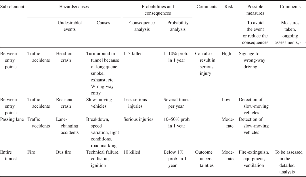
The form used to document the risk analysis is often standardised. An example of an analysis form for a risk analysis of a road tunnel is shown in Table 6.1. We see from the table that the risk is described by using categories. The categories cover possible undesirable events, along with the probability and expected consequence if such an event should occur. We see from the table that, in the case of a bus fire, we expect that there will be 10 people killed. The number can be 0, 1 or 30, but the expectation is 10.

Table 6.1 Example of an analysis form for a coarse risk analysis of a road tunnel

In stating probabilities, terms such as often and seldom should be avoided as they are open to different interpretations. A better alternative is to say directly what we mean, for example, % probability that an event will occur within the period of 1 year. Some people will perhaps say that it is difficult for the analysis group to express that there is a % probability or a % probability, for example. The answer to this is ‘yes’, it can be difficult to assign probabilities. However, it does not help ‘hiding’ behind expressions such as ‘often’ or ‘seldom’ without explaining what one means by these terms. Also, the consequence categories should be precisely defined, rather than using terms such as high, low and so on.

A coarse risk analysis is often combined with other analysis methods. The coarse analysis identifies the most important risk contributors, and then the causal picture and/or the consequence picture can be assessed in detail using more detailed analyses.

Example: workplace accidents

The working environment committee at the Packing Factory Ltd has found that in the bag department, which has about 90 employees, the number of injuries is too high. The committee therefore decides to implement some injury preventive measures to reduce the injury rate in the department. It is, however, not clear where such measures should be directed and which measures would most effectively prevent injuries. Opinions in the working environment committee differ widely.

In the bag department, production is a series production of large, multiple ply paper bags. Each production line comprises several machines. The raw material is paper rolls. The main operator task in the department is to monitor and adjust the machines. Some operators deal with manual handling of products. It is the operators who are operating the machines that are most exposed to injuries.

The working environment committee instructs the safety delegate of the company to work out a basis for decisions on preventing measures. The safety delegate is familiar with risk analyses and uses such an analysis to establish the desired decision basis.

By means of the risk analysis, the safety delegate will identify possible injuries that might occur in the department, where they might occur, possible causes and the severity of the injuries. Table 6.2 presents a summary of the analysed hazards. With respect to probability/frequency, the following classification is used:

1. 1. Very unlikely: less than once per 1000 years (yearly probability 1:1000)
2. 2. Unlikely: once per 100 years (yearly probability 1:100)
3. 3. Quite likely: once per 10 years (yearly probability 1:10)
4. 4. Likely: once per year
5. 5. Frequently: once per month or more frequently.

Table 6.2 Summary of identified hazards

No	Event	Cause	Consequence	Probability	Consequence category
1.	Crushing in cutting machinery	Hand in running machine, e.g., due to inattention	Finger/hand injury	4	III
2.	Crushing in pulling machinery	As in 1	Finger/hand injury	4	III
3.	Crushing at intermediate station	As in 1	Finger/hand injury	3	III
4.	Damage at guillotine	As in 1	Finger/hand injury	3	III
5.	Being caught at the glue station	Inattention	Hand/arm injury	3	III
6.	Being caught in folding station	Missing cover inattention	Significant body injuries	3	IV
7.	Crushing between rollers	As 1	Finger/hand injury	4	III
8.	Damage from machinery splinter	Rupture during operation	Major wounds	4	II
9.	Knocks from edge, machine part, etc.	Inattention	Wounds, cuts	4	I
10.	Hair or clothes being caught between rollers	Inattention	Significant body injuries	2	IV
11.	Bodily damage from unobserved machinery start-up	Technical failure, noise, inattention	Significant body injuries	2	IV
12.	Crushing when lifting roll	Inattention	Finger/hand injuries	4	III
13.	Damage due to roll coming loose	Rupture of spindle, carelessness	Severe injuries, fatalities	2	V
14.	Damage due to dropping roll	Failure of tackle, inadequate fastening	Severe injuries, fatalities	4	V
15.	Paper fire	Ignition of paper dust oil, weld sparks, smoking	Loss of casings/sacks, destruction of machines	3	I

Also for the consequences five categories are used:

1. I. Does not result in injuries
2. II. Minor injuries
3. III. Major injuries
4. IV. Death or total disability
5. V. Death or total disability for several persons.

The starting point for the hazard identification was the injury reports for the whole department for the last 9 years. Data on near misses were also available. In addition, the system description was studied to identify other hazards. For the hazards based on the injury reports, the classification is based on this statistics. For example, two injuries caused by crushing in the cutting machinery are registered. This gives a classification ‘likely’. Judgement has been used for the hazards that are not based on the injury statistics.

In Figure 6.1, the hazards have been placed in a consequence probability diagram. The consequence categories are marked along the horizontal axis with consequences increasing to the right. Similarly, frequency/probability is marked along the vertical axis, with frequency increasing downwards. The following conclusions are drawn:

• Highest risk: hazard number 14, which equals ‘paper roll falls from tackle’
• Other contributors to high risk are: events that include crushing and catching in the machinery.

The events with the lowest risk are numbers 9 and 15. Thus, in general, for this type of consequence probability diagram, the events with the highest risk are those in the bottom right corner, whereas the events with the lowest risk are placed in the upper left corner. We should, however, be very careful when drawing conclusions from the matrix since it is based on a rough classification and is based a probability–consequence description only, not for example expressing the strength of knowledge on which the assignments are based.

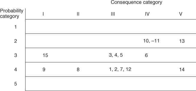
Figure 6.1 Probability (frequency)–consequence diagram.

Note that hazard 15 (paper fire) has low risk in relation to personnel. If we focus on material assets or economic values, this hazard would contribute much more to risk.

Based on the risk analysis, the safety delegate can now identify and rank measures to prevent accidents, as a basis for the decision-making on which measures to implement.

6.2 Job safety analysis

A job safety analysis is a simple qualitative risk analysis methodology used to identify the hazards that are associated with a work assignment that is to be executed. A job safety analysis is usually checklist-based. Normally, the persons planning/executing the work assignment are part of the analysis team. By carrying out a job safety analysis, we ensure the following:

• It is clarified whether the work assignment is a ‘standard’ operation that can be carried out according to procedures and normal practice or whether it is a non-standard case that requires special measures or studies. The latter case may lead to postponement until more detailed studies are carried out.
• Possible conflicts between different jobs may be identified; for example, painting and welding jobs close to each other at the same time.
• The persons carrying out the work assignment will think through what they should do and consider each work assignment in a risk-related perspective. The mere act of thinking through and planning the work assignments can, in itself, be a risk-reducing measure.
• What can go wrong at the various steps of the job will be assessed. Through this process, those carrying out the job will become aware of the most risky aspects of the work assignment, and adequate risk-reducing measures can then be implemented.

A job safety analysis is carried out by dividing the job into a number of sub-jobs or tasks and then performing an analysis for each task. The division into tasks is illustrated by the following example:

1. Change of a car wheel
   1. 1. Set the hand brake.
   2. 2. Take out the spare wheel from the boot.
   3. 3. Check the air pressure.
   4. 4. Remove the hub cap.
   5. 5. Ensure that the jack fits and is stable.
   6. 6. Jack up the car, but not so much that the wheels leave the ground.
   7. 7. Loosen the wheel nuts.
   8. 8. Jack up the car further, but not more than is necessary.
   9. 9. Remove the wheel and so on.

The identification of hazards includes a check of the following:

• What type of injuries that may occur, for example, crushing?
• Are special problems or deviations likely to occur?
• Is the task difficult or uncomfortable to carry out?
• Are there alternative ways of carrying out the task?

The identified hazards are assessed and the conclusions categorised, for example, in the following way:

1. 0 insignificant risk
2. 1 acceptable risk; actions unnecessary
3. 2 the risk should be reduced
4. 3 the risk must be reduced; there is a need for immediate actions.

When evaluating the risk and the need for actions/risk-reducing measures, considerations should be given to, for example:

• violation of statutory requirements;
• violation of requirements set by the company;
• high risk documented by means of accident statistics;
• high energy concentration;
• unreasonable requirements with respect to attention and vigilance for the operator;
• low tolerance for human errors in the technical system;
• whether the solution of the problem is known and available.

Special sheets have been developed for job safety analysis. Such sheets will typically include the following main points:

• Description of the job
• Accident experience (statistics)
• Accident potential
• Requirements
• Job sequence (tasks)
• Risk assessment
• Actions/measures.

Often, the sheets include a list of possible actions that are to be considered. The actions may, for example, be related to improved equipment and tools, better work instructions, improved education and training and so on.

6.3 Failure modes and effects analysis

Failure Modes and Effects Analysis (FMEA) is an analysis method to reveal possible failures and to predict the failure effects on the system as a whole. The method is inductive; for each component of the system, we investigate what happens if this component fails. The method represents a systematic analysis of the components of the system to identify all significant failure modes and to see how important they are for the system's performance. Only one component is considered a time, and the other components are then assumed to function perfectly. FMEA is therefore not suitable for revealing critical combinations of component failures.

FMEA was developed in the 1950s and was one of the first systematic methods used to analyse failures in technical systems. The method has appeared with different names and with somewhat different content. If we describe or rank the criticality of the various failures in the FMEA, the analysis is often referred to as an FMECA (Failure Modes, Effects and Criticality Analysis). The criticality is a function of the failure effect and the frequency/probability as seen below. The difference between an FMEA and an FMECA is not distinct, and in this book, we do not distinguish between these two methods. In the following, we also use the term FMEA when the analysis includes a description/ranking of criticality.

In several enterprises, it is nowadays a requirement that an FMEA be included as part of the design process and that the results from the analysis be part of the system documentation.

To ensure a systematic study of the system, a specific FMEA form is used. The FMEA form may, for example, include the following columns:

1. Identification (column 1). Here the specific component is identified by a description and/or number. It is also common to refer to a system drawing or a functional diagram.

   Function, operational state (column 2). The function of the component, that is, its working tasks in the system, is briefly described.

   The state of the component when the system is in normal operation, is described, for example, whether it is in a continuous operation mode or in a stand-by mode.

   Failure modes (column 3). All the possible ways the components can fail to perform its function are listed in this column. Only the failure modes that can be observed from ‘outside’ are included. The internal failure modes are to be considered as failure causes. These causes can possibly be listed in a separate column. In some cases, it will also be of interest to look at the basic physical and chemical processes that can lead to failure (failure mechanisms), such as corrosion.

   Often we also state how the different failure modes of the component are detected and by whom.

   Example: In a chemical process plant, a specific valve is considered as a component in the system. The function of the valve is to open and close on demand. ‘The valve does not open on a demand’ and ‘the valve does not close on a demand’ are relevant failure modes, as well as ‘the valve opens when not intended’ and ‘the valve closes when not intended’. However, ‘washer bursts’ is an example of a cause of a specific failure mode.

2. Effect on other units in the system (column 4). In those cases where the specific failure mode affects other components in the system, this is stated in this column. Emphasis should be given to identification of failure propagation, which does not follow the functional chains of the functional diagrams. For example, increased load on the remaining pillars that are supporting a common load when a pillar collapses; vibration in a pumping house may induce failure of the driving unit of the pump and so on.
3. Effect on system (column 5). In this column, we describe how the system is influenced by a specific failure mode. The operational state of the system as a result of failure is to be expressed, for example, whether the system is in the operational state, changed to another operational mode or not in an operational state.
4. Corrective measures (column 6). Here, we describe what has been done or what can be done to correct the failure, or possibly to reduce the consequences of the failure. We may also list the measures that are aimed at reducing the probability that failure will occur.
5. Failure frequency (column 7). In this column, we state the assigned frequency (probability) for a specific failure mode and consequence. Instead of presenting frequencies for all the different failure modes, we may give a total frequency and relative frequencies (in percentages) for the different failure modes.
6. Failure effect ranking (column 8). A failure is ranked according to its effect with respect to reliability and safety, possibilities of mitigating the failure, length of the repair time, production loss and so on. We might, for example, use the following grouping of failure effects:
   1. Small: A failure that does not reduce the functional ability of the system more than normally is accepted.
   2. Large: A failure that reduces the functional ability of the system beyond the acceptable level, but the consequences can be corrected and controlled.
   3. Critical: A failure that reduces the functional ability of the system beyond the acceptable level and that creates an unacceptable condition, either operational or with respect to safety.

   Remarks (column 9). Here we state, for example, assumptions and suppositions.

   By combining the failure frequency (probability) and the failure effect (consequence), the criticality of a specific failure mode is determined.

Example: storage tank

Figure 6.2 shows a tank that functions as a buffer storage for the transport of fluid from the source to the consumer. The consumption of fluid is not constant, and the liquid level will therefore vary. The control of avoiding overfilling of the buffer storage is automatic and can be described as follows: when the liquid level reaches a certain height—‘normal high’, then the Level Switch High (LSH) will be activated and LSHH sends a closure signal to valve V1. The fluid supply to the tank then stops. If this mechanism does not function, and the liquid level continues to increase to ‘abnormally high level’, then the Level Switch High High (LSHH) will be activated and LSHH sends a closure signal to valve V2. The fluid supply to tank then stops. At the same time, the LSHH sends an opening signal to valve V3 so that the fluid is drained. The draining pipe has higher capacity than that of the supply pipe.

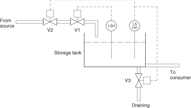
Figure 6.2 Storage tank example.

A simple FMEA has been carried out for this system. Tables 6.3 and 6.4 show the completed forms for the components LSH, LSHH, V1, V2 and V3. The following ranking of the failure effects is used:

1. 1. There is no fluid supply.
2. 2. The fluid in the tank is drained.
3. 3. The liquid level may increase to an abnormal height.
4. 4. The tank is overfilled if valve V1 does not close.

The consequence categories are crude. For example, there is no indication of the length of a stop in the fluid supply. Only failure modes related to the normal operational state have been included. For example, the failure mode ‘does not open’ is not included for valves V1 and V2.

Table 6.3 Completed FMEA form for storage tank example components LSH, LSHH and V1

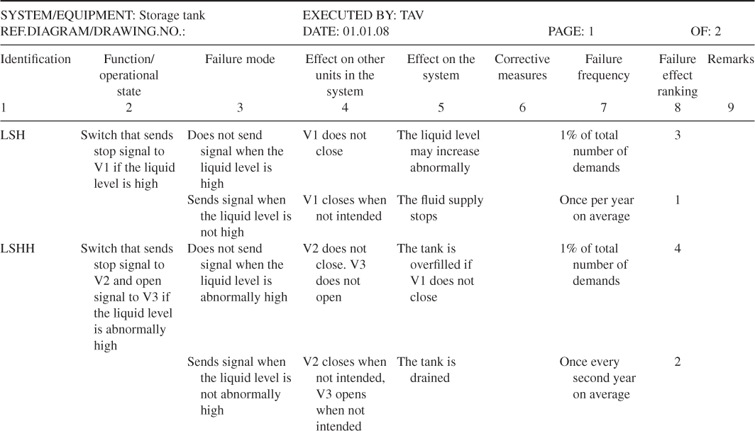
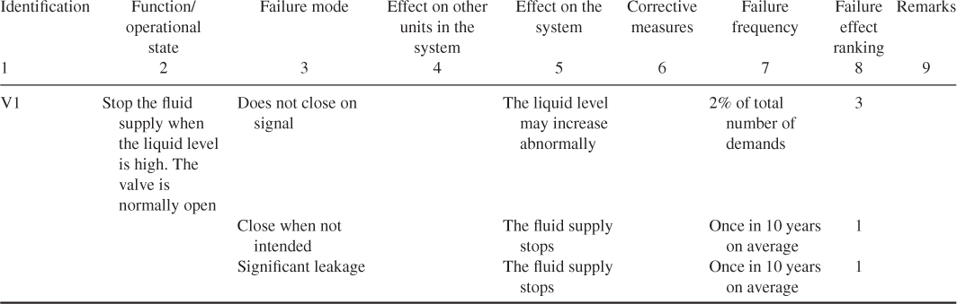
Table 6.4 Completed FMEA form for storage tank example components V2 and V3

Now, what are the results of the analysis? First, the analysis of the relevant components has given a good understanding of the type of component failures that might occur and their effects. The analysis demonstrates that the system has a high reliability. The probability that tank is overfilled is small. The component LSHH seems to be the most critical component in the system. We return to the criticality issue in Section 6.6.

6.3.1 Strengths and weaknesses of an FMEA

The strong points of the FMEA are that it gives a systematic overview of the important failures in the system and it forces the designer to evaluate the reliability of his/her system. In addition, it represents a good basis for more comprehensive quantitative analyses, such as fault tree analyses and event tree analyses. Of course, an FMEA gives no guarantee that all critical component failures have been revealed. Through a systematic review such as FMEA, most weaknesses of the system as a result of individual component failures will, however, be revealed.

In an FMEA, the attention is, in many cases, mostly on technical failures, whereas human failure contributions are often overlooked. This may, to some extent, be compensated by including the human functions as components in the system.

An FMEA can be unsuitable for analysing systems with much redundancy (several components that can perform the same function such that failure of one unit does not result in system failure). In such systems, it will not be so interesting to analyse individual component failures, since these cannot directly affect the function of the system. The interest is then focused on combinations of two or more events that together can cause system failure. The storage tank example shows, however, that an FMEA can give valuable information about the possible failures and their effects also for a system with some redundancy. The storage tank system is redundant in that to avoid overfilling of the tank, it is sufficient that valve 1 closes, or that valve 2 closes or valve 3 opens. The analysis is a good starting point for a fault tree analysis or an event tree analysis.

Perhaps the main disadvantage of using the FMEA method is that all components are analysed and documented, also the failures of little or no consequences. An FMEA can therefore be very demanding. The amount of documentation can be extensive. This problem can be reduced by proper component definitions. For the storage tank system, we could have defined the system components by the different parts of valves V1, V2 and V3, and the level switches LSH and LSHH. This would, however, have increased the extent of the analysis considerably, without obtaining more insights into possible undesirable events at the system level. For larger systems, it may be an advantage to define subsystems (system functions). An initial FMEA may be related to failures of these subsystems. Detailed FMEA studies can then be carried out for specific subsystems.

The standard FMEA does not address the strength of knowledge as discussed in Section 2.4, but the method (and the methods considered in the following sections) can easily be adjusted to also cover this aspect.

6.4 Hazard and operability studies

Hazard and Operability (HAZOP) studies is a qualitative risk analysis technique that is used to identify weaknesses and hazards in a processing facility; it is normally used in the planning phase (design). The HAZOP technique was originally developed for chemical processing facilities, but it can also be used for other facilities and systems. For example, it is widely used in Norway in the oil and gas industry.

A HAZOP study is a systematic analysis of how deviation from the design specifications in a system can arise and an analysis of the risk potential of these deviations. Based on a set of guidewords, scenarios that may result in a hazard or an operational problem are identified. The following guidewords are commonly used: NO/NOT, MORE OF/LESS OF, AS WELL AS, PART OF, REVERSE and OTHER THAN. The guidewords are related to process conditions, activities, materials, time and place. For example, when analysing a pipe from one unit to another in a process plant, we define the deviation ‘no throughput’ based on the guideword NO/NOT and the deviation ‘higher pressure than the design pressure’ based on the guideword MORE OF. Then causes and consequences of the deviation are studied. This is done by asking questions. For example, for the first-mentioned deviation in the pipe example above, the following questions would be asked:

• What must happen to ensure the occurrence of the deviation ‘no throughput’ (cause)?
• Is such an event possible (relevance/probability)?
• What are the consequences of no throughput (consequence)?

As a support in the work of formulating meaningful questions based on the guidewords, special forms have been developed.

The principle that is used in a HAZOP study can be illustrated in the following way:

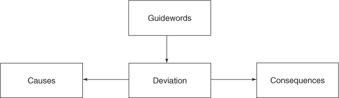
In a HAZOP study, worksheets are used to document deviations, causes, consequences and recommendations/decisions. These worksheets are to be considered as a type of FMEA forms.

A HAZOP study is undertaken by a group of personnel led by a HAZOP leader. The leader should be experienced in using the technique, but does not necessarily need to have thorough knowledge about the actual process. The group comprises persons who have detailed knowledge about the system to be analysed. Typically, the group will consist of five to six persons, in addition to the HAZOP leader.

Through a HAZOP study, critical aspects of the design can be identified, which requires further analysis. Detailed, quantitative reliability and risk analyses will often be generated in this way.

A HAZOP study of a planned plant will, in the same way as an FMEA, normally be most useful if the analysis is undertaken after the Process and Instrumentation Diagrams (PI&Ds) have been worked out. It is at this point in time that sufficient information about the way the plant is to be operated is available.

A HAZOP study is a time- and resource-demanding method. Nevertheless, the method has been widely used in connection with the review of the design of process plants for a safer, more effective and reliable plant.

6.5 SWIFT

Structured What-If Technique (SWIFT) is a risk analysis method in which one uses the lead question—What if—systematically in order to identify deviations from normal conditions. The method is similar to HAZOP in the sense that it utilises a pre-defined checklist of the elements that are to be reviewed. SWIFT is, however, somewhat more flexible than HAZOP, and the checklist can be easily adapted to the application. In a SWIFT analysis, the checklist is reviewed, and we ask, ‘what if’ the individual elements on the checklist should occur. In this way, hazardous situations, accident events and so on can be identified. An example of a checklist is shown in Table 6.5.

Table 6.5 Example of a checklist for use in SWIFT analyses

Question categories	Examples
Material problems	Flammability, reactivity, toxicity and so on
External effects/impacts	Natural effects (e.g. wind)
	Human-made effects (e.g. falling loads)
Operational failures/human errors	Information, time/sequence, organisation and so on
Supervisory errors/measurement errors	Testing, measurement, management and so on
Equipment/instrument failures	Pumps, valves, computers, power supply and so on
Wrong set-up	Omissions, concurrent operations and so on
Auxiliary system failures	Cooling, fire-fighting water supply, ventilation, communication and so on
Loss of integrity/capacity	Wear and tear, maintenance, overload and so on
Emergency operations	Fire, explosion, toxic spills and so on

The analysis is carried out in a manner similar to that used in HAZOP by an analysis team that typically has a variety of competencies, for example, in design, operations, maintenance, safety and so on. In the analysis, possible problems and combinations of conditions that can be problematic are described, and possible risk-reducing measures are identified.

6.6 Fault tree analysis

The fault tree analysis method was developed by Bell Telephone Laboratories in 1962 when they performed a safety evaluation of the Minuteman Launch Control System. The Boeing company further developed the technique and made use of computer programmes for both qualitative and quantitative fault tree analysis. Since the 1970s fault tree analysis has become widespread and is today one of the most used reliability and risk analysis methods. Its applications are found in most industries. The space industry and the nuclear power industry have perhaps been the two industries that have used fault tree analysis the most.

A fault tree is a logical diagram that shows the relation between system failure, that is, a specific undesirable event, for example, the initiating event of the bow-tie or the failure of a system barrier, and failures of the components of the system. The undesirable event constitutes the top event of the tree and the different component failures constitute the basic events of the tree. For example, for a production process, the top event might be that the process stops, and one basic event might be that a particular motor fails. A basic event does not necessarily represent a pure component failure; it may also represent human errors or failures that are due to external loads, such as extreme environmental conditions. A fault tree comprises symbols that show the basic events of a system, and the relation between these events and the state of the system. The graphical symbols that show the relation are called logical gates. The output from a logical gate is determined by the input states. The graphical symbols vary somewhat depending on the standard that is used. Figure 6.3 shows the most important symbols in a fault tree together with the interpretations of the symbols.

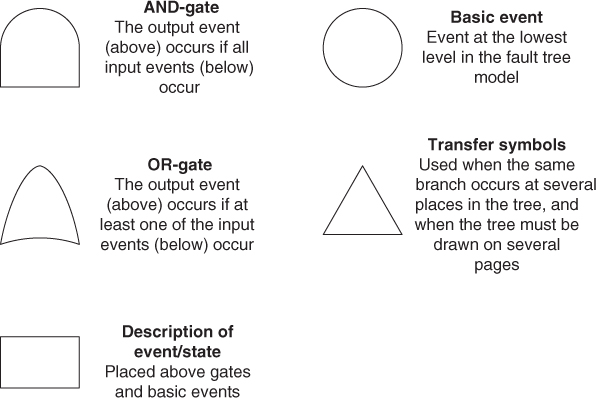
Figure 6.3 Fault tree symbols.

A fault tree that comprises only AND and OR gates can alternatively be represented by a reliability block diagram. This is a logical diagram showing the functional ability of a system. Each component in the system is illustrated by a rectangle as shown in Figure 6.4.

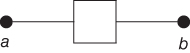
Figure 6.4 Functional element in a reliability block diagram.

If there is connection from a to b in Figure 6.4, this means that the component is functioning based on the criteria that apply for the particular analysis. Usually, ‘functioning’ means absence from one or more failure modes. A presentation of some equivalent fault trees and reliability block diagrams is shown in Figure 6.5.

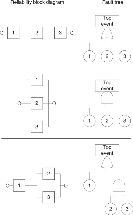
Figure 6.5 Correspondence between reliability block diagrams and fault trees.

The top event is the starting point when constructing the fault tree. Next, we must identify the possible failures (events) that can be the direct causes of the top event. These events are linked to the top event by a logical gate. Then, we work successively down to the basic events on the component level. The analysis is deductive and is carried out by repeatedly asking: ‘How can this happen?’ or ‘What are the causes of this event?’ The development of the causal sequence is stopped when we have reached the desired level of the detail. It is essential to ‘think locally’ and to develop the fault tree by using a step-by-step approach. Avoid gate-to-gate connections, that is, connecting one gate directly to the next without providing an intermediate event in between. A common mistake in fault tree construction is over-rapid development of one branch of a tree without proceeding down level by level systematically (tendency to want to reach the basic events too rapidly and not to use broad sub-event descriptions).

Example: tank storage

We consider the tank system described in Section 6.3. The task now is to construct a fault tree for the system with the top event ‘overfilling of the tank’ and basic events corresponding to failures of the components V1, V2, V3, LSH and LSHH. Figure 6.6 shows a fault tree for this top event, with an associated reliability block diagram (Figure 6.7). Note that we disregard the possibility of failure of the transfer of signals from LSH to V1 and from LSHH to V2 and V3.

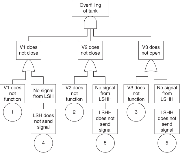
Figure 6.6 Fault tree for the top event ‘overfilling of the tank’.

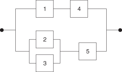
Figure 6.7 Reliability block diagram for the fault tree in Figure 6.6.

6.6.1 Qualitative analysis

A fault tree gives valuable information about which failure combinations that can result in an undesirable event. Such a failure combination is called a cut set:

A cut set in a fault tree is a set of basic events the occurrence of which ensure that the top event occurs. A cut set is minimal if it cannot be reduced and still ensures the occurrence of the top event.

For the corresponding reliability block diagram, this definition is equivalent to:

A cut set is a combination of components the failures of which ensure that the system fails. A cut set is minimal if it cannot be reduced without losing its status as a cut set.

For simple fault trees, the minimal cut sets can be determined directly from the fault tree or from the associated reliability block diagram. In most cases, it would be most convenient to use the reliability block diagram. For more complex fault trees, there is a need for an algorithm. The most known computer-based algorithm is MOCUS (Rausand and Høyland 2004).

Example (cont'd)

The minimal cut sets for the tree in Figure 6.6 are determined directly from the fault tree or its associated reliability diagram:

{1,5}, {4,5}, {1,2,3}, {2,3,4}.

A qualitative analysis of the fault tree is based on an identification of the minimal cut sets. Since system failure occurs when all the events in at least one minimal cut sets occur, the system can be viewed as a series structure of the minimal cut-parallel structures, as shown in Figure 6.8.

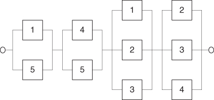
Figure 6.8 The minimal cut set representation of the system in Figure 6.7.

The number of events in a cut set is called the order of the cut set. The minimal cut sets are ranked according to their order. It may be argued that single-event cut sets (single jeopardy) are highly undesirable as only one failure can lead to the top event, two-event cut sets (double jeopardy) are better and so on. Further ranking based on human errors and active/passive equipment failure is also common. The qualitative approach is however potentially misleading. It may be that larger cut sets have a higher failure probability than smaller ones; this requires a quantitative analysis. Common-cause failures are due to a single event affecting multiple events in the fault tree. This might be a power failure miscalibrating all sensors. Less obviously, elements such as common manufacturer, common location and so on may also lead to common-cause failures.

6.6.2 Quantitative analysis

If we can determine probabilities for the basic events of the fault tree, then we can perform a quantitative analysis. Usually, we would like to calculate

• the probability that the top event will occur;
• the importance (criticality) of the basic events (components) of the tree.

To compute the top event probability, it is common to use the following approximation method: for each minimal cut set, compute the probability that it fails and then sum over all minimal cut sets.

Example (cont'd)

Again we look at the tank example, see the fault tree in Figure 6.6. Assume that the probabilities of the basic events are as given in the FMEA, that is, 2%, 2%, 2%, 1% and 1%. Then using the representation in Figure 6.8, we find that the probability that the top event ‘overfilling of the tank’ will occur is approximately equal to

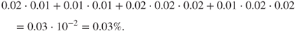
This means that if the liquid level increases and reaches a high level about 25 times a year, then the probability of overfilling of the tank during a 1-year period would be approximately 0.75% (). The percentage can be viewed as a risk index for the activity. We are allowed to sum the unreliabilities for the 25 cases because the probability that the top event will occur two or more times during 1 year is negligible compared to 0.75%.

We see from these calculations of the probability of the top event that the component 5 (LSHH) is the most important component from a reliability point of view, in the sense that the probability of the top event would be reduced the most by an improvement in the reliability of this component.

The approximation produces accurate results if the probability of the top event is small and the basic events are independent. The basic events are independent if the probability that a basic event will occur does not depend on whether one or more of the other basic events have occurred. Using this approximation method, we disregard the possibility that two or more minimal cut sets will be in the failure state at the same time. For this particular example, the error term is negligible. Alternatively, we can carry out an exact computation, using the fact that the system is a combination of series and parallel structures. The calculations go like this (refer to Appendix B). The components are judged independent. Let be the probability that component functions as required, and let . We refer to and as the reliability and unreliability of component , respectively. Components 1 and 4 are in series; hence, the reliability of this substructure is . Components 2 and 3 are in parallel, and, hence, the unreliability of this substructure is . Combining this substructure and component 5 gives a series structure having reliability . This structure is again in parallel with the structure of components 1 and 4, and we find that the unreliability of the system is equal to

This exact formula gives an unreliability of 0.03% as above.

Some final remarks concerning the fault tree analysis: the fault tree is easy to understand for persons with no prior knowledge about the technique. The fault tree analysis is well documented and simple to use. One of the advantages of using the technique is that the persons undertaking the analysis is forced to understand the system. Many weak points in the system are revealed and corrected already in the construction phase of the tree. The fault tree analysis gives a static ‘picture’ of the failure combinations that can cause the top event tooccur. The fault tree analysis method is not suitable for analysing systems with dynamic properties. Another problem is treatment of common-mode failures.

There exist many other methods for cause analysis. We would like to mention the cause-and-effect analysis (also called Ishikawa diagram), which has some similarities to the fault tree analysis but is less structured and does not have the same two-state restriction as a fault tree (Rausand and Høyland 2004). The cause-and-effect analysis is not suited for quantitative analyses.

6.7 Event tree analysis

An event tree analysis is used to study the consequences of the initiating event of a bow-tie diagram. What type of event sequences (scenarios) can the initiating event produce? The method may be used both qualitatively and quantitatively. In the former case, the method provides a picture of the possible scenarios. In the latter case, probabilities are linked to the various event sequences and their consequences.

An event tree analysis is carried out by posing a number of questions where the answer is either ‘yes’ or ‘no’. See the simple example in Figure 6.9. We may interpret the tree as follows: a gas leakage may occur, and depending on the events (ignition) and (escalation), the outcome becomes , or , where represents the number of fatalities or costs (or both). The number of gas leakages in a time interval is denoted . If an initiating event occurs, it leads to fatalities if both the events and occur, if the event occurs and the event does not occur, and if the event does not occur. Here, is equal to zero if and do not occur and so on.

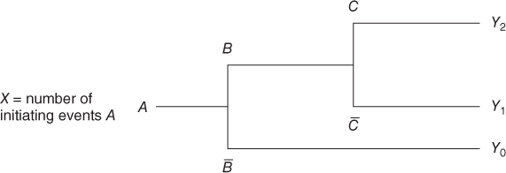
Figure 6.9 Event tree example. Here means ‘not ’ and so on.

From the tree branches, a set of scenarios are generated, as shown by the aforementioned example. It is common to pose the branch questions in such a way that the ‘desired’ answer is either up (yes) or down (no) for all the branch questions. In this way, the ‘best’ scenario will come out at one end and the worst scenario, at the other end. If we have many branch questions, we will end up with a large number of event sequences. Often, many of these are almost identical, and it is common to group the various event sequences prior to processing them further in the risk analysis.

The branch questions can be divided into two main categories:

1. 1. Those related to physical phenomena such as explosions and fires
2. 2. Those related to barriers in the system, such as a fire-fighting system.

Often, the event tree analysis covers both categories. If we wish to reflect the use of various risk-reducing measures, category 2 should be highlighted.

The next step in the analysis will be to draw up a so-called consequence matrix, which describes the consequences arising from each terminating event or group of terminating events. In Figure 6.9, the consequences are restricted to the number of fatalities () and/or costs. The matrix is generated by considering categories of losses. For fatalities we use categories 0, 1 and 2, and for costs categories , say. The maximum number of fatalities is two in this case.

For each scenario , we need to specify the consequences. This can either be done by using a fixed number, say 2, or expected values, for example, the expected number of fatalities ( say), or alternatively by determining a probability distribution for the possible outcome categories, for example, 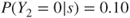, and .

If probabilities are assigned for branch questions, then a probability can be determined for each terminating event (scenario) by multiplying the probabilities for events in the chain. Let us look at the example of Figure 6.9. Here,

and unconditionally

We have assumed that is small so that we can ignore the probability of two or more events during the time interval considered. In the case of more frequent events, we can use the formula

It is important to be aware that all the probabilities are conditioned on the earlier events in the event sequence. The probability of two fatalities is not the same in scenario as in scenario .

To simplify the analysis, it is common to assume that the outcome is fixed for a specific scenario, and in the following, we assume that , and . Whether this new model is sufficiently accurate has to be evaluated of course.

Suppose that we arrive at a probability , either using modelling or a direct argument using experience data and knowledge about the phenomena and system in question.

Similarly, we determine a probability . Let us suppose that we arrive at . Then, we can calculate the probability distribution for the number of fatalities . Approximation formulae such as

6.1

are used, which are utilising the probability that the event two or more ignited leakages in 1 year has a negligible probability compared to that of one ignited leakage. Suppose that . We then obtain and and a FAR value equal to

assuming 8760 hours of exposure per year for two persons. Remember that the Fatal Accident Rate (FAR) value is defined as the expected number of fatalities per 100 million exposed hours.

6.7.1 Barrier block diagrams

There exist several alternative tools to event trees. Some of the examples are event sequence diagrams and barrier block diagrams. The former is much in use, for example, in the aviation and aerospace industries. We will not discuss it in any further detail in this book. Barrier diagrams are widely used, for example, in the Norwegian oil and gas industry. By this approach, initiating events, barrier functions and terminating events are shown along a horizontal line. The barrier systems are shown as boxes below this line; see the example in Figure 8.1. Barrier functions are functions to prevent the occurrence of an initiating event or to reduce the damage by interrupting an undesirable event sequence. Barrier systems are solutions that will ensure that the actual barrier function is carried out. One of the strengths of barrier block diagrams is that they clearly show the difference between barrier functions and barrier systems.

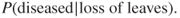
6.8 Bayesian networks

A Bayesian network consists of events (nodes) and arrows. The arrows indicate dependencies, that is, causal connections. Each node can be in various states; the number of states is selected by the risk analyst. A Bayesian network is not limited to two states, as are event trees and fault trees. In a quantitative analysis, we must determine conditional probabilities for these states given the causal connections. This can be done by a direct argument or using some type of specified procedures. A simple Bayesian network is presented in Figure 6.10. This example will be used to explain what a Bayesian network is and how it is used. The example was obtained from the software supplier Hugin.

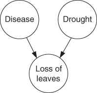
Figure 6.10 Example of a Bayesian network.

Example

John has an apple tree in the garden and one day he discovers that the tree is losing its leaves. He knows that apple trees can lose their leaves if they are not adequately watered. But it can also be an indication of a disease.

The network in Figure 6.10 models the causal links. The network consists of three nodes: disease, drought and loss of leaves. As a simplification, each node has two states only; the apple tree is either diseased or not, it is impacted by drought or not and it is either losing leaves or not. We see from the arrows in the Bayesian network that disease and drought are possible causes of the tree losing its leaves. It is common to use the designation ‘parent’ and ‘child’ for the two different levels of the nodes in the network. For the three nodes in the example, we will thus say that ‘disease’ and ‘drought’ are the parent nodes for ‘loss of leaves’. A quantitative analysis requires that we specify the conditional probabilities. This is often done in tables called CPT or Conditional Probability Tables. The probabilities that the tree will lose leaves, given various combinations of disease and drought, are given in Table 6.6.

Table 6.6 Conditional probabilities

	Drought Yes		Drought No
	Disease Yes %	Disease No %	Disease Yes %	Disease No %
Loss of leaves Yes	95	85	90	2
Loss of leaves No	5	15	10	98

The probabilities could be based on available experience data or determined by expert judgements. All probabilities in Table 6.6 are conditioned on the state of the parent nodes. In addition, we need to specify the unconditional probabilities for disease and drought. Let us assume that John, after consulting a botanist, specifies a probability of 10% that the tree is diseased. He also assigns a probability of 10% that the tree is suffering from drought.

We have thus constructed a Bayesian network and established the probabilities for the various quantities (events) in the network. The task is now to calculate the probability of the apple tree being diseased, given that we have observed that it is losing leaves, or in other words,

To find this probability, we make use of the so-called Bayes' formula. To simplify, we introduce events , and , expressing disease (), drought () and loss of leaves (). The complementary events are denoted and so on. The task is to compute .

Bayes' formula gives

where has been assigned the value 0.10. Hence, it remains to determine and . Let us first look at .

The arrows in the Bayesian network show that in addition to being dependent on , is also dependent on . Using the law of total probability, we can write

Assuming independence between and (in line with the network model shown in Figure 6.10), we obtain

Hence, according to Bayes' formula . Similarly, we obtain , as

By summing and , we obtain .

We can then compute the desired probability:

In other words, there is a 49% probability that the tree is diseased when we see that it is losing leaves.

Bayesian networks can be used for many types of applications, for example:

• Shipping accidents: Modelling of what causes the responsible officer on a ship to make an error leading to a collision. Factors such as the time of day, stress, experience, knowledge, shift arrangements and weather are factors that may be considered in the cause modelling.
• Financial considerations: Credit assessments of customers. Factors that are deemed to influence the capacity to pay, such as age and income, are modelled. In discussions with customers, individual nodes are locked, the model is updated and a probability of the customer not being able to pay within a given period is calculated.
• Medicine: Assistance in making diagnoses. A model for the relationship between various symptoms and analysis results is drawn up (once by experts within the profession). Subsequently, other physicians may submit analysis results and symptoms for individual patients into the model (lock some of the nodes) and calculate the probability of the patient having a disease or being healthy.

Bayesian networks have been regularly used in fields such as the aviation and aerospace industries, but have not been very common in, for example, the offshore industry. We see, however, that the method is becoming more and more commonly used in a number of different fields, such as offshore operations, health, transport, banking and financial areas.

Bayesian networks have been shown to be appropriate in connection with analyses of complex causal relationships. In risk analyses, however, there will always be a need for simple methods such as event and fault trees. Obviously, different situations call for different methods.

6.9 Monte Carlo simulation

Monte Carlo simulation represents an alternative to analytical calculation methods. The technique is to generate a computer model of the system to be investigated, for example, represented as a reliability block diagram, and then to simulate the operation of the system for a specific period of time. Using the computer, we generate realisations of the system performance. The sojourn times in the various states are determined by sampling from appropriate probability distributions. For example, for a two-state component, the operating times (uptimes) are sampled from a lifetime distribution and the downtimes are sampled from a repair time distribution. If represents the lifetime of a component, the probability distribution is given by ; see Appendix B. The system state is computed and logged as time elapses. For each realisation of the system performance, we can compute, for example, the uptime of the system. Simulating the system performance a number of times, say times, we can estimate the probability distribution for the uptime and the probability that the system is functioning at a particular point in time. For example, the probability is estimated by the average value of the realisations where the system is functioning. By increasing , the estimation error can be made negligible.

With a Monte Carlo simulation model, the time aspect is more easily handled than with an analytical method. A Monte Carlo simulation model may be a fairly good representation of the real world. This is one of the greatest attractions of Monte Carlo simulation over analytical methods.

Monte Carlo Simulation requires in general detailed input data. For example, the lifetime and repair time distributions must be specified. Mean values, as used in many analytical models, are not sufficient. On the other hand, the output from a Monte Carlo simulation model is very extensive and informative.

The main disadvantage of the Monte Carlo simulation technique compared with an analytical approach is the time and expense involved in the development and execution of the model. To obtain accurate results using simulation, a large number of trials is usually required, especially when the system is functioning most of the time. The time and expense aspect is very important if the model is to be used to study the effects of changes in system configurations, or if sensitivity analyses are to be performed.

With a complex Monte Carlo simulation model, it is difficult to check if the program has been written correctly and, therefore, if the result can be relied upon. For further details on Monte Carlo simulation, see Zio (2013).