10.10. Two-Dimensional Jets

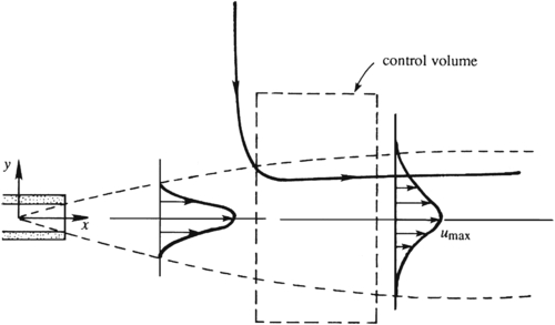
The previous nine sections have considered boundary layers over solid surfaces. The concept of a boundary layer, however, is more general, and the approximations involved are applicable whenever the vorticity in the flow is confined in thin layers, even in the absence of a solid surface. Such a layer can be in the form of a jet of fluid ejected from an orifice, a wake (where the velocity is lower than the upstream velocity) behind a solid object, or a thin shear layer (vortex sheet) between two uniform streams of different speeds. As an illustration of the method of analysis of these free shear flows, we shall consider the case of a laminar two-dimensional jet, which is an efflux of fluid from a long and narrow orifice that issues into a large quiescent reservoir of the same fluid. Downstream from the orifice, some of the ambient fluid is carried along with the moving jet fluid through viscous vorticity diffusion at the outer edge of the jet (Figure 10.30). The process of drawing reservoir fluid into the jet by is called entrainment.

The velocity distribution near the opening of the jet depends on the details of conditions upstream of the orifice exit. However, because of the absence of an externally imposed length scale in the downstream direction, the velocity profile in the jet approaches a self-similar shape not far from where it emerges into the reservoir, regardless of the velocity distribution at the orifice.

For large Reynolds numbers, the jet is narrow and the boundary-layer approximation can be applied. Consider a control volume with sides cutting across the jet axis at two sections (Figure 10.30); the other two sides of the control volume are taken at large distances from the jet axis. No external pressure gradient is maintained in the surrounding fluid so dp/dx is zero. According to the boundary-layer approximation, the same zero pressure gradient is also impressed upon the jet. There is, therefore, no net force acting on the surfaces of the control volume, and this requires the x-momentum flux at the two sections across the jet to be the same.

Figure 10.30 Simple laminar two-dimensional free jet. A narrow slot injects fluid horizontally with an initial momentum flux J (per unit span) into a nominally quiescent reservoir of the same fluid. The region of horizontally moving fluid slows and expands as x increases. A typical streamline showing entrainment of surrounding fluid is indicated.

Let u₀(x) be the stream-wise velocity on the x-axis and assume Re = u₀x/ν is sufficiently large for the boundary-layer equations to be valid. The flow is steady, two-dimensional (x, y), without body forces, and with constant properties (ρ, μ). Then ∂/∂y ≫ ∂/∂x, v ≪ u, ∂p/∂y = 0, so the fluid equations of motion are the same as for the Blasius boundary layer: (7.2) and (10.18). However, the boundary conditions are different here:

u=0fory→±∞andx>0,

(10.53)

v=0ony=0forx>0,and

(10.54)

u=u˜(y)onx=x0,

(10.55)

where u˜ is a known flow profile. Now partially follow the derivation of the von Karman boundary-layer integral equation. Multiply (7.2) by u and add it to the left side of (10.18) but this time integrate over all y to find:

∫−∞+∞2u∂u∂xdy+∫−∞+∞[u∂v∂y+v∂u∂y]dy=∫−∞+∞∂τ∂ydy,orddx∫−∞+∞u2dy+[uv]−∞+∞=[τ]−∞+∞.

(10.56)

Since u(y = ±∞) = 0, all derivatives of u with respect to y must also be zero at y = ±∞. Thus, since τ = μ(∂u/∂y), the second and third terms in the second equation of (10.56) are both zero. Hence, (10.56) reduces to:

ddx∫−∞+∞u2dy=0,

(10.57)

a statement that the stream-wise momentum flux is conserved. Thus, when integrated, (10.57) becomes:

∫−∞+∞u2dy=const.=∫−∞+∞u˜2(y)dy=J/ρ,

(10.58)

where the second equality follows from (10.55). Here, the constant is the momentum flux in the jet per unit span, J, divided by the fluid density, ρ.

A similarity solution is obtained far enough downstream so that the boundary-layer equations are valid and u˜(y) has been forgotten. Thus, we can seek a solution in the form of (9.32) or (10.19):

ψ=u0(x)δ(x)f(η),whereη=y/δ(x),δ(x)=[νx/u0(x)]1/2,

(10.59)

and u₀(x) is the stream-wise velocity on y = 0. The stream-wise velocity throughout the field is obtained from differentiation:

u=∂ψ/∂y=[νxu0(x)]1/2(df/dη)[νx/u0(x)]−1/2=u0(x)(df/dη).

(10.60)

The final equality here implies that f′ = 1 on η = 0. When (10.60) is substituted into (10.58), the dependence of u₀(x) on x is determined:

Jρ=∫−∞+∞u2dy=u02(x)∫−∞+∞f′2(η)dy=u02(x)δ(x)∫−∞+∞f′2(η)dη.

(10.61)

Since the integral is a dimensionless constant (=C), we must have:

Cuo2(x)δ(x)=Cuo3/2(x)·(νx)1/2=J/ρ,

so:

u0(x)=[J2/C2ρ2νx]1/3,andδ(x)=[Cρν2x2/J]1/3.

(10.62, 10.63)

Thus, (10.59) becomes:

ψ=[Jνx/Cρ]1/3f(η)whereη=y/[Cρν2x2/J]1/3.

(10.64)

In terms of the stream function, (10.18) becomes:

∂ψ∂y∂∂x(∂ψ∂y)−∂ψ∂x∂∂y(∂ψ∂y)=ν∂2∂y2(∂ψ∂y).

(10.65)

Evaluating the derivatives using (10.64) and simplifying produces a differential equation for f:

3f‴+f″f+f′2=0.

The boundary conditions for x > 0 are:

f′=0forη→±∞,f′=1onη=0,andf=0onη=0.

(10.66, 10.67, 10.68)

Integrating the differential equation for f once produces:

3f″+f′f=C1.

Evaluating at η = ±∞ implies C₁ = 0 from (10.66) since f′ = 0 implies f′′= 0 too. Integrating again yields:

3f′+f2/2=C2.

(10.69)

Evaluating on η = 0 implies C₂ = 3 from (10.67) and (10.68). The independent and dependent variables in (10.69) can be separated and integrated:

3dfdη=3−f22or∫df1−f2/6=∫dη.

The integral on the left in the second equality can be evaluated via the variable substitution f=6tanhβ, and leads to:

tanh−1(f6)=η6+C3,orf=6tanh(η6+C3).

(10.70)

Evaluating the final expression on η = 0 implies C₃ = 0 from (10.68). Thus, using (10.60), (10.62), and (10.70), the stream-wise velocity field is:

u(x,y)=u0(x)f′(η)=(J2C2ρ2νx)1/3sech2(y6[JCρν2x2]1/3),

(10.71)

and the dimensionless constant, C, is determined from:

C=∫−∞+∞f′2(η)dη=∫−∞+∞sech4(η6)dη=463.

(10.72)

The mass flux of the jet per unit span is:

m˙=∫−∞+∞ρu0(x)f′(η)dy=ρu0(x)δ(x)∫−∞+∞f′(η)dη=ρu0(x)δ(x)[f]−∞+∞=ρu0(x)δ(x)·26.

Using (10.62), (10.63), and (10.72), this simplifies to:

m˙=(36Jρ2νx)1/3,

(10.73)

which shows that the jet's mass flux increases with increasing downstream distance as the jet entrains ambient reservoir fluid via the action of viscosity. The jet's entrainment induces flow toward the jet within the reservoir. The vertical velocity is:

v=−∂ψ∂x=−13(JνCρx2)1/3[f−2ηf′],orvu0(x)=−[f−2ηf′]3RexwhereRex=xu0(x)ν.

(10.74)

Here, f(η)→±6 and 2ηf′(η)=2ηsech2(η/6)→0 as η → ±∞, so:

vu0(x)→∓63Rexasη→±∞.

(10.75)

Thus, the jet's entrainment field is a flow of reservoir fluid toward the jet from above and below.

The jet spreads as it travels downstream, and this can be deduced from (10.71). Following the definition of δ₉₉ in Section 10.2, the 99% half width of the jet, h₉₉, may be defined as the y-location where the horizontal velocity falls to 1% of its value at y = 0. Thus, from (10.71) we can determine:

sech2(h996[JCρν2x2]1/3)=0.01→h996[JCρν2x2]1/3≅2.2924→h99≅5.6152[Cρν2x2J]1/3,

(10.76)

which shows the jet width grows with increasing downstream distance like x^2/3. Viscosity increases the jet's thickness but higher momentum jets are thinner. The Reynolds numbers based on the stream-wise (x) and cross-stream (h₉₉) dimensions of the jet are:

Rex=xu0(x)ν=(3Jx46ρν2)2/3andReh99=h99u0(x)ν=5.6152(3Jx46ρν2)1/3.

Unfortunately, this steady-flow, two-dimensional laminar jet solution is not readily observable because the flow is unstable when Re ≫ 1. The low critical Reynolds number for instability of a jet or wake is associated with the existence of one or more inflection points in the stream-wise velocity profile, as discussed in Chapter 11. Nevertheless, the laminar solution has revealed at least two significant phenomena – constancy of jet momentum flux and increase of jet mass flux through entrainment – that also apply to round jets and turbulent jets. However, the cross-stream spreading rate of a turbulent jet is found to be independent of Reynolds number and is faster than the laminar jet, being more like h₉₉ ∝ x rather than h₉₉ ∝ x^2/3 (see Chapter 12).

A second example of a two-dimensional jet that also shares some boundary-layer characteristics is the wall jet. The solution here is due to Glauert (1956). We consider fluid exiting a narrow slot with its lower boundary being a planar wall taken along the x-axis (see Figure 10.31). Near the wall (y = 0) the flow behaves like a boundary layer, but far from the wall it behaves like a free jet. For large Re_x the jet is thin (δ/x ≪ 1) so ∂p/∂y ≈ 0 across it. The pressure is constant in the nearly stagnant outer fluid so p ≈ const. throughout the flow. Here again the fluid mechanical equations of motion are (7.2) and (10.18). This time the boundary conditions are:

u=v=0ony=0forx>0,andu(x,y)→0asy→∞.

(10.77, 10.78)

Figure 10.31 The laminar two-dimensional wall jet. A narrow slot injects fluid horizontally along a smooth flat wall. As for the free jet, the thickness of the region of horizontally moving fluid slows and expands as x increases but with different dependencies.

Here again, a similarity solution valid for Re_x → ∞ can be found under the assumption that the initial velocity distribution is forgotten by the flow. However, unlike the free jet, the momentum flux of the wall jet is not constant; it diminishes with increasing downstream distance because of the wall shear stress. To obtain the conserved property in the wall jet, integrate (10.18) in the wall normal direction from y to ∞:

∫y∞u∂u∂xdy+∫y∞v∂u∂ydy=ν∫y∞∂2u∂y2dy=ν[∂u∂y]y∞=−ν∂u∂y,

multiply this by u, and integrate from 0 to ∞ in the wall normal direction:

∫0∞(u∂∂x∫y∞u22dy)dy+∫0∞(u∫y∞v∂u∂ydy)dy=−ν2∫0∞∂u2∂ydy=−ν2[u2]0∞=0.

The final equality follows from the boundary conditions (10.77) and (10.78). Integrating the interior integral of the second term on the left by parts and using (7.2) yields a term equal to the first term and one that lacks any differentiation:

∫0∞(u∂∂x∫y∞u2dy)dy−∫0∞u2vdy=0.

(10.79)

Now consider:

ddx∫0∞(u∫y∞u2dy)dy=∫0∞(∂u∂x∫y∞u2dy)dy+∫0∞(u∂∂x∫y∞u2dy)dy,

use (7.2) in the first term on the right side, integrate by parts, and combine this with (10.79) to obtain:

ddx∫0∞(u∫y∞u2dy)dy=0.

(10.80)

This says that the flux of exterior momentum flux remains constant with increasing downstream distance and is the necessary condition for obtaining similarity exponents.

As for the steady free laminar jet, the field equation is (10.65) and the solution is presumed to be in the similarity form specified by (10.59). Here u₀(x) is to be determined and this similarity solution should be valid when x ≪ x_o, where x_o is the location where the initial condition is specified, which we take to be the upstream extent of the validity of the boundary-layer momentum equation (10.18) or (10.65). Substituting u = ∂ψ/∂y = u₀(x)f′(η) from (10.59) into (10.80) produces:

ddx[u03(x)·νxu0(x)∫0∞(f′∫η∞f′2dη)dη]=0.

(10.81)

If the double integration is independent of x, then the factor outside the integral must be constant.

Therefore, set xu02(x)=C2, which implies u0(x)=Cx−1/2 so (10.59) becomes:

ψ(x,y)=[νCx1/2]1/2f(η)whereη=y/δ(x),δ(x)=[νx3/2/C]1/2,

(10.82)

After appropriately differentiating (10.82), substituting into (10.65), and canceling common factors, (10.65) reduces to:

f‴+ff″+2f′2=0,

subject to the boundary conditions (10.77) and (10.78): f(0) = 0; f′(0) = 0; f′(∞) = 0. This third-order equation can be integrated once after multiplying by the integrating factor f, to yield 4ff″−2f′2+f2f′=0, where the constant of integration has been evaluated at η = 0. Dividing by the integrating factor 4f3/2 allows another integration. The result is:

f−1/2f′+f3/2/6=C1≡f∞3/2/6,wheref∞=f(∞).

The final integration can be performed by separating variables and defining g2(η)=f/f∞:

∫dff∞3/2f−f2=16∫dη,or∫dg1−g3=f∞12∫dη.

The integration on the left may be performed via a partial fraction expansion using 1−g3=(1−g)·(1+g+g2) with the final result left in implicit form:

−ln(1−g)+3tan−1(2g+13)+ln(1+g+g2)1/2=f∞4η+3tan−1(13),

(10.83)

where the boundary condition g(0) = 0 was used to evaluate the constant of integration. The profiles of f and f′ are plotted vs. η in Figure 10.32. We can verify easily that f′ → 0 exponentially fast in η from this solution for g(η). As η → ∞, g → 1, so for large η the solution for g reduces to −ln(1−g)+3tan−13+(1/2)ln3≅f∞η/4+3tan−1(1/3). The first term on each side of this equation dominates, leaving 1−g≈e−(f∞/4)η. Thus, for η → ∞, we must have: f′=2f∞gg′≈12f∞2exp[−f∞η/4]. The mass flow rate per unit span in the steady laminar wall jet is:

m˙=∫0∞ρudy=ρu0(x)δ(x)∫0∞f′(η)dη=ρνCf∞x1/4,

(10.84)

indicating that entrainment increases the mass flow rate in the jet with x^1/4. The two constants, C and f_∞, can be determined from the integrated form of (10.81) in terms of Ψ, the flux of the exterior momentum flux (a constant):

u02(x)νx∫0∞(f′∫η∞f′2dη)dη=C2ν∫0∞(f′∫η∞f′2dη)dη=Ψ,

(10.85)

and knowledge of m˙ at one downstream location.

Figure 10.32 Variation of normalized mass flux (f) and normalized stream-wise velocity profile (f′) with similarly variable η for the laminar two-dimensional wall jet. Reprinted with the permission of Cambridge University Press.

The entrainment into the steady laminar wall jet is evident from the form of v=−∂ψ/∂x=−νC(f−3ηf′)/4x3/4, which simplifies to v ≈ −νCf∞/4x3/4 as η → ∞, so, far above the jet, the flow is downward toward the jet.