13.3. Equations of Motion for Geophysical Flows
From Section 4.7, the equations of motion for a stratified fluid, observed in a system of coordinates rotating at a constant angular velocity Ω with respect to the “fixed stars” are:
 (4.10, 13.2, 4.9)
where F is the friction force per unit mass of fluid, the centrifugal acceleration is combined into the body force acceleration gez (see Section 4.7), and diffusive effects in the density equation are omitted. This equation set embodies the Boussinesq approximation, discussed in Section 4.9, in which the density variations are neglected everywhere except in the gravity term and the vertical scale of the motion is assumed less than the “scale height” of the medium c2/g, where c is the speed of sound. This assumption is very good in the ocean, in which c2/g∼200 km. In the atmosphere it is less applicable, because c2/g∼10 km. Under the Boussinesq approximation, the principle of mass conservation is expressed by ∇ · u = 0  (4.10), and the density equation Dρ/Dt = 0 (4.9) follows from the non-diffusive heat or species equation DT/Dt = 0 or DS/Dt = 0 and an incompressible equation of state of the form δρ/ρ0 = −αδT or δρ/ρ0 = βδS, where S the concentration of a constituent such as water vapor in the atmosphere or the salinity in the ocean. Fortunately, (4.9) and (4.10) are consistent with each other, as described in Section 4.2, even if they occur together here for a different reason.
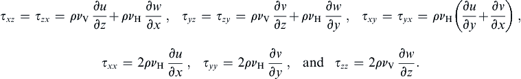
(4.10), and the density equation Dρ/Dt = 0 (4.9) follows from the non-diffusive heat or species equation DT/Dt = 0 or DS/Dt = 0 and an incompressible equation of state of the form δρ/ρ0 = −αδT or δρ/ρ0 = βδS, where S the concentration of a constituent such as water vapor in the atmosphere or the salinity in the ocean. Fortunately, (4.9) and (4.10) are consistent with each other, as described in Section 4.2, even if they occur together here for a different reason.For a closed set of equations, the friction force per unit mass, F in (13.2), must be appropriately related to the (average) velocity field. Geophysical flows are commonly turbulent and anisotropic with vertical velocities that are typically much smaller than horizontal ones. From Section 4.5, the friction force is given by Fi = ∂τij/∂xj, where τij is the viscous stress tensor. In large-scale geophysical flows, however, the frictional forces are typically provided by turbulent momentum exchange and viscous effects are negligible. Yet, the complexity of turbulence makes it impossible to relate the stress to the (average) velocity field in a simple way. Thus, to proceed in a rudimentary manner that includes anisotropy, the eddy viscosity hypothesis (12.115) is adopted but the turbulent viscosity is presumed to have directional dependence. In particular, geophysical fluid media are commonly in the form of stratified layers that inhibit vertical transport of horizontal momentum. This means that the exchange of momentum upward or downward across a horizontal surface is much weaker than that in either horizontal direction across a vertical surface. To reflect this phenomenology in F, the vertical eddy viscosity νV is assumed to be much smaller than the horizontal eddy viscosity νH, and the turbulent stress components are assumed to be related to the fluid velocity u = (u, v, w) by:
 (13.3)
There are two difficulties with the set (13.3). First, the expressions for τxz and τyz depend on the rotation of fluid elements in a vertical plane and not just their deformation. As stated in Section 4.5, a requirement for a constitutive equation for a fluid is that the stresses should be independent of fluid element rotation and should depend only on element deformation. Therefore, τxz should depend only on the combination (∂u/∂z+∂w/∂x), whereas the expression in (13.3) depends on both deformation and rotation. A tensorially correct geophysical treatment of the frictional terms is discussed, for example, in Kamenkovich (1967). Second, the eddy viscosity assumption for modeling momentum transport in turbulent flow is of questionable validity (Pedlosky (1971) describes it as a “rather disreputable and desperate attempt”). However, (13.3) provides a simple approximate formulation for viscous effects suitable for the current level of inquiry. So, using the set (13.3) and further assuming νV and νH are constants, the components of the frictional force Fi = ∂τij/∂xj become:
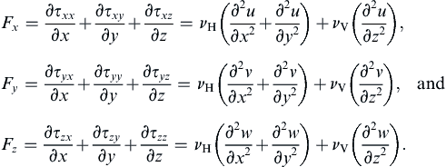 (13.4)
Estimates of the eddy coefficients vary greatly. Typical suggested values are νV∼10 m2/s and νH∼105 m2/s for the lower atmosphere, and νV∼0.01 m2/s and νH∼100 m2/s for the upper ocean. In comparison, the molecular values are ν = 1.5 × 10⁻⁵ m2/s for air and ν = 10−6 m2/s for water at atmospheric pressure and 20°C.
When (13.4) is used in (13.2), the set (4.9), (4.10) and (13.2) provides five equations for the five field variables u, v, w, p, and ρ. However, for most geophysical flows, these five equations are commonly solved after several additional simplifications and approximations.
In general, geophysical flow problems should be solved using spherical polar coordinates attached to earth. However, the vertical scales of the ocean and the troposphere are of order 5 to 15 km while their horizontal scales are of order of hundreds, or even thousands, of kilometers. Thus, the trajectories of fluid elements in atmospheric and oceanic flows are nearly horizontal, |u|, |v| ≫ |w|, and most geophysical flows can be considered to occur in thin layers. In fact, (4.10) suggests that:
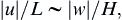
where H is the vertical scale and L is the horizontal length scale. Stratification and Coriolis effects usually constrain the vertical velocity to be even smaller than |u|H/L. If, in addition, the horizontal length scales of interest are much smaller than the radius of the earth (= 6371 km), then the curvature of the earth can be ignored, and the motion can be studied by adopting a local Cartesian system on a tangent plane. Figure 13.3 shows this tangent-plane xyz coordinate system: with x increasing eastward (into the page), y northward, and z upward. The corresponding velocity components are u (eastward), v (northward), and w (upward).

Figure 13.3 Tangent-plane Cartesian coordinates. The x-axis points into the plane of the paper. The y-axis is tangent to the earth's surface and points toward the north pole. The z-axis is vertical, opposing gravity. The earth's angular rotation vector has positive y and z components in the northern hemisphere. The angle θ is the geographic latitude and is defined with respect to the local surface normal; thus, it is not quite the same as the geocentric latitude indicated near the center of the figure.
The tangent-plane approximation allows the components of the Coriolis acceleration in (13.2) to be evaluated. The earth rotates at a rate:

around the polar axis, in a counterclockwise sense looking from above the north pole. From Figure 13.3, the components of angular velocity of the earth in the local tangent-plane Cartesian system are Ω = (Ωx, Ωy, Ωz) = (0, Ω cos θ, Ω sin θ), where θ is the geographic latitude. If the earth were perfectly spherical, θ would be the geocentric latitude as well. With this geometry, the Coriolis acceleration appearing in (13.2) is:
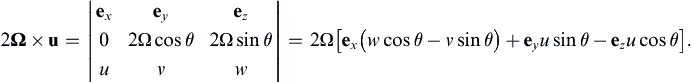
The thin-fluid layer approximation, |w| ≪ |v|, allows w cos θ to be ignored compared to v sin θ in the term multiplied by ex away from the equator (θ = 0). Thus, the three components of the Coriolis acceleration are:
 (13.5, 13.6)
is twice the local vertical component of Ω. Since vorticity is twice the angular velocity, f is referred to as the planetary vorticity, or, more commonly, as the Coriolis parameter or the Coriolis frequency. It is positive in the northern hemisphere and negative in the southern hemisphere, varying from ±1.45 × 10⁻⁴ s−1 at the poles to zero at the equator. This makes sense, since an object at the north pole spins around a vertical axis at a counterclockwise rate Ω, whereas a object at the equator does not spin around a vertical axis. The quantity, Ti = 2π/f, is called the inertial period, for reasons that will be clear in Section 13.9; it does not represent the components of a vector.
The pressure and gravity terms in (13.2) can also be simplified by writing them in terms of the pressure and density perturbations from a state of rest:
 (13.7)
where the static distribution of density, ρ ¯ ( z )  , and pressure,
 p ¯ ( z )  , follow the hydrostatic law (1.14). When (13.7) is substituted into (13.2), the first two terms inside parentheses on the right side become:
, and pressure, , follow the hydrostatic law (1.14). When (13.7) is substituted into (13.2), the first two terms inside parentheses on the right side become: (13.8)
because the terms in [,]-braces sum to zero from (1.14).
In addition, the vertical component of the Coriolis acceleration, namely −2Ωu cos θ, is generally negligible compared to the dominant terms in the vertical equation of motion, namely g ρ ′ / ρ 0  and
and ρ 0 − 1 ( ∂ p ′ / ∂ z )  . Thus, combining (13.2), (13.4), (13.5), (13.6), and (13.8) while ignoring −2Ωu cos θ in the vertical momentum equation, leads to the simplified equation set: (4.9), (4.10):
and . Thus, combining (13.2), (13.4), (13.5), (13.6), and (13.8) while ignoring −2Ωu cos θ in the vertical momentum equation, leads to the simplified equation set: (4.9), (4.10):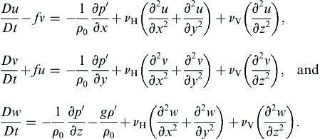 (13.9)
These are the equations for primarily horizontal fluid motion within a thin layer on a locally-flat rotating earth. Note that only the vertical component of the earth’s angular velocity appears as a consequence of the flatness of the fluid trajectories.
f-Plane Model
The Coriolis parameter f = 2Ω sin θ clearly varies with latitude θ. However, this variation is important only for phenomena having very long time scales (several weeks) or very long length scales (thousands of kilometers). For many purposes, f can be well approximated as constant, say f0 = 2Ω sin θ0, where θ0 is the central latitude of the region under study. A model using a constant Coriolis parameter is called an f-plane model.
β-Plane Model
The variation of f with latitude can be approximately represented by expanding (13.6) in a Taylor series about the central latitude θ0:
 (13.10)
Here, df/dθ = 2Ωcosθ and dθ/dy = 1/R, where R = 6371 km is the radius of the earth. A model that takes into account the variation of the Coriolis parameter in the simplified form given by the final quality of (13.10) with β as constant is called a β-plane model.
Example 13.3
Compute the magnitude of the vertical Coriolis acceleration for a 185 km/hr (100 knot) horizontal air speed at latitude 45°. What temperature fluctuation in an air mass at 300 K would produce an equivalent buoyant acceleration? Is neglect of the vertical Coriolis acceleration likely to be justified in most situations? Explain.
Solution
For the given speed and latitude, the magnitude of the vertical Coriolis acceleration is:

The vertical (or buoyant) acceleration term in the final equation of the set (13.9) is gρ′/ρ0. For constant air pressure, temperature and density fluctuations are related by δT/T0 = –δρ/ρ0, so an equivalent buoyant acceleration is will be produced by a temperature fluctuation T′ that satisfies:

In this case, with T0 = 300 K, T′ is just 0.16 K. Thus, as long as naturally occurring temperature fluctuations are several degrees Kelvin or more, the vertical Coriolis acceleration can be neglected in a simplified analysis involving this wind speed. However, a 100-knot wind represents an extreme situation; near the ground it corresponds to category-three hurricane force winds while aloft it corresponds to a strong jet stream. Thus, neglect of the vertical Coriolis acceleration is likely to be well justified in more ordinary atmospheric situations.