13.16. Geostrophic Turbulence

Two common modes of instability of a large-scale wind or current system were presented in the preceding sections. When the flow is strong enough, such instabilities can cause a flow to become chaotic or turbulent. A peculiarity of large-scale turbulence in the atmosphere or the ocean is that it is essentially two dimensional in nature. The existence of the Coriolis acceleration, stratification, and the relatively small thickness of geophysical media severely restricts the vertical velocity in large-scale flows, which tend to be quasi-geostrophic, with the Coriolis acceleration balancing the horizontal pressure gradient to the lowest order. Because vortex stretching, a key mechanism by which ordinary three-dimensional turbulent flows transfer energy from large to small scales, is absent in two-dimensional flow, one expects that the dynamics of geostrophic turbulence are likely to be fundamentally different from that of three-dimensional, laboratory-scale turbulence discussed in Chapter 12. However, such motion can still be considered turbulent because it is unpredictable and diffusive.

A key result on the subject was discovered by the meteorologist Fjortoft (1953), and since then Kraichnan, Leith, Batchelor, and others have contributed to various aspects of the problem. A good discussion is given in Pedlosky (1987), to which the reader is referred for a fuller treatment. The present discussion merely highlights a few important results.

In two-dimensional turbulence, the vorticity, ζ, normal to the plane of fluid motion is of special interest and its mean square value, ζ2¯, is known as enstrophy. In an isotropic turbulent field we can define an energy spectrum S(K) so that:

u2¯=∫0∞S(K)dK,

where K is the magnitude of the wave number. It can be shown that the enstrophy spectrum is K²S(K), so that:

ζ2¯=∫0∞K2S(K)dK,

which makes sense because vorticity involves the spatial derivatives of velocity.

Consider a freely evolving turbulent field in which the shape of the velocity spectrum changes with time. The large scales are essentially inviscid, so that both energy and enstrophy are conserved (or nearly so):

ddt∫0∞S(K)dK≅0,andddt∫0∞K2S(K)dK≅0,

(13.143, 13.144)

where terms proportional to the molecular viscosity v have been neglected on the right-hand sides of these equations. Enstrophy conservation is unique to two-dimensional turbulence because of the absence of vortex stretching.

Suppose that the energy spectrum initially contains all its energy at wave number K₀. Nonlinear interactions transfer this energy to other wave numbers, so that the sharp spectral peak smears out. For the sake of argument, suppose that all of the initial energy goes to two neighboring wave numbers K₁ and K₂, with K₁ < K₀ < K₂. Conservation of energy and enstrophy requires that:

S(K0)=S(K1)+S(K2)andK02S(K0)=K12S(K1)+K22S(K2).

From this we can find the ratios of energy and enstrophy spectra after the transfer:

S(K1)S(K2)=K2−K0K0−K1K2+K0K1+K0,andK12S(K1)K22S(K2)=K12K22K22−K02K02−K12.

(13.145)

As an example, suppose that nonlinear smearing transfers energy to wave numbers K₁ = K₀/2 and K₂ = 2K₀. Then (13.145) shows that S(K₁)/S(K₂) = 4 and K12S(K1)/K22S(K2) = 1/4, so that more energy goes to lower wave numbers (large scales), whereas more enstrophy goes to higher wave numbers (smaller scales). This important result for two-dimensional turbulence was derived by Fjortoft (1953). Clearly, the constraint of enstrophy conservation in two-dimensional turbulence has prevented a symmetric spreading of the initial energy peak at K₀.

The unique character of two-dimensional turbulence is evident here. In three-dimensional turbulence, the primary topic of Chapter 12, the energy goes to smaller and smaller scales until it is dissipated by viscosity. In geostrophic turbulence, on the other hand, the energy goes to larger scales, where it is less susceptible to viscous dissipation. Numerical calculations are indeed in agreement with this behavior and show that energy-containing eddies grow in size by coalescing. On the other hand, the vorticity becomes increasingly confined to thin shear layers on the eddy boundaries; these shear layers contain very little energy. The backward (or inverse) energy cascade and forward enstrophy cascade are represented schematically in Figure 13.34. It is clear that there are two inertial regions in the spectrum of a two-dimensional turbulent flow, namely, the energy cascade region and the enstrophy cascade region. If energy is injected into the system at a rate ε, then the energy spectrum in the energy cascade region has the form S(K)∝ε^2/3K^−5/3; the argument is essentially the same as in the case of the Kolmogorov spectrum in three-dimensional turbulence (Section 12.7), except that the transfer is (backward) to lower wave numbers. A dimensional argument also shows that the energy spectrum in the enstrophy cascade region is of the form S(K)∝α^2/3K⁻³, where α is the forward enstrophy flux to higher wave numbers. There is negligible energy flux in the enstrophy cascade region.

As the eddies grow in size, they become increasingly immune to viscous dissipation, and the inviscid assumption implied in (13.143) becomes increasingly applicable. (This would not be the case in three-dimensional turbulence in which the eddies continue to decrease in size until viscous effects drain energy out of the flow.) In contrast, the corresponding assumption in the enstrophy conservation equation (13.144) becomes less and less valid as enstrophy goes to smaller scales, where viscous dissipation drains enstrophy out of the system. At later stages in the evolution, then, (13.144) may not be a good assumption. However, it can be shown (see Pedlosky, 1987) that the dissipation of enstrophy actually intensifies the process of energy transfer to larger scales, so that the red cascade (that is, transfer to larger scales) of energy is a general result of two-dimensional turbulence.

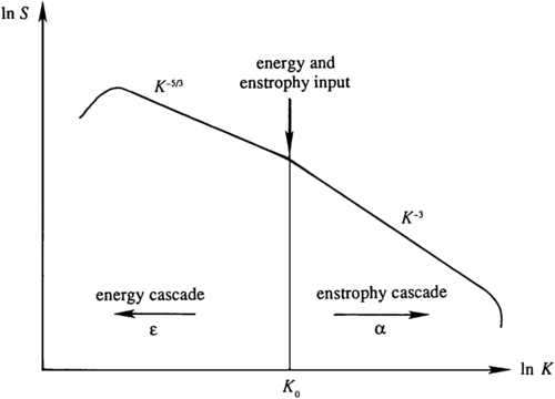
Figure 13.34 Energy and enstrophy cascade in two-dimensional turbulence. Here the two-dimensional character of the turbulence causes turbulent kinetic energy to cascade to larger scales, while enstrophy cascades to smaller scales.

The eddies, however, do not grow in size indefinitely. They become increasingly slower as their length scale l increases, while their velocity scale u remains constant. The slower dynamics makes them increasingly wavelike, and the eddies transform into Rossby-wave packets as their length scale becomes of order (Rhines, 1975):

l∼u/β(Rhineslength),

where β = df/dy and u is the rms fluctuating speed. The Rossby-wave propagation results in an anisotropic elongation of the eddies in the east–west (“zonal”) direction, while the eddy size in the north–south direction stops growing at u/β. Finally, the velocity field consists of zonally directed jets whose north–south extent is of order u/β. This has been suggested as an explanation for the existence of zonal jets in the atmosphere of the planet Jupiter (Williams, 1979). The inverse energy cascade regime may not occur in the earth’s atmosphere and the ocean at mid-latitudes because the Rhines length (about 1000 km in the atmosphere and 100 km in the ocean) is of the order of the internal Rossby radius, where the energy is injected by baroclinic instability. (For the inverse cascade to occur, u/β needs to be larger than the scale at which energy is injected.)

Eventually, however, the kinetic energy has to be dissipated by molecular effects at the Kolmogorov microscale η, which is of the order of a few millimeters in the ocean and the atmosphere. A fair hypothesis is that processes such as internal waves drain energy out of the mesoscale eddies, and breaking internal waves generate three-dimensional turbulence that finally cascades energy to molecular scales.

Example 13.14

Equations (13.145) describe the reverse energy cascade of geostropic turbulence in spectral terms. Redo this analysis by considering the merger of two large-scale cyclones idealized as identical disks of air with radius r_o rotating as solid bodies with rate Ω_o. Estimate the radius r_f and rotation rate Ω_f of the final cyclone if it also rotates as a solid body. How are these answers changed if half of the enstrophy is lost during the merger?

Solution

For an atmosphere of height H, the kinetic energy of one disk of air with radius r_o undergoing solid body rotation with rate Ω_o is:

12∫volumeρ|u|2dV=12∫0Hρ∫0ro(Ωor)22πrdrdz=π4ρ¯oHΩo2ro4.

 

where ρ¯o is the altitude-averaged density. Thus, conservation of energy for two such disks merging into one implies:

2·π4ρ¯oHΩo2ro4=π4ρ¯oHΩf2rf4.

 

The vorticity inside each of the two initial disks is 2Ω_o, so conservation of enstrophy requires:

2·πro2A(2Ωo)2=πrf2A(2Ωf)2.

 

where A is the relevant horizontal area for averaging the square of the vorticity. Simultaneous solution of these two equations leads to:

rf=roandΩf=2Ωo.

 

Thus, the single merged cyclone is the same size as the original two but it rotates more quickly. From a spectral point of view, this merger represents a reduction in the wave number – even though the merged cyclone is the same size – because the final flow field contains one cyclonic event in a nominal horizontal distance of A^1/2 while the initial field contained two cyclonic events in the same distance.

When only half the enstrophy survives the merging process, the prior steps may be redone to find that the final cyclonic disk is larger and rotates slower that either of the original cyclonic disks.

rf=2roandΩf=Ωo/2.