As mentioned in the introductory section of this chapter, turbulence rapidly dissipates kinetic energy, and an understanding of how this happens is possible via a term-by-term inspection of the equations that govern the kinetic energy in the mean flow and the average kinetic energy of the fluctuations.
An equation for the mean-flow's kinetic energy per unit mass, E¯=12Ui2, can be obtained by multiplying (12.30) by Ui, and averaging (Exercise 12.15). With Sij¯=12(∂Ui/∂xj+∂Uj/∂xi) defining the mean strain-rate tensor, the resulting energy-balance or energy-budget equation for E¯ is:
The left side is merely the total time derivative of E¯ following a mean-flow fluid particle, while the right side represents the various mechanisms that bring about changes in E¯.
The first three divergence terms on the right side of (12.46) represent transport of mean kinetic energy by pressure, viscous stresses, and Reynolds stresses. If (12.46) is integrated over the volume occupied by the flow to obtain the rate of change of the total (or global) mean-flow kinetic energy, then these transport terms can be transformed into a surface integral by Gauss’ theorem. Thus, these terms do not contribute to the total rate of change of E¯ if Ui = 0 on the boundaries of the flow. Therefore, these three terms only transport or redistribute mean-flow kinetic energy from one region to another; they do not generate it or dissipate it.
The fourth term is the product of the mean flow's viscous stress (per unit mass) 2νS¯ij and the mean strain rate S¯ij. It represents the direct viscous dissipation of mean kinetic energy via its conversion into heat.
The fifth term is analogous to the fourth term. It can be written as uiuj¯(∂Ui/∂xj)=uiuj¯S¯ij so that it is a product of the turbulent stress (per unit mass) and the mean strain rate. Here, the doubly contracted product of a symmetric tensor uiuj¯ and the tensor ∂Ui/∂xj is equal to the product of uiuj¯ and the symmetric part of ∂Ui/∂xj, namely S¯ij, as proved in Section 2.10. If the mean flow is given by U(y) alone, then uiuj¯(∂Ui/∂xj)=uv¯(dU/dy). From the preceding section, uv¯ is likely to be negative if dU/dy is positive. Thus, the fifth term is likely to be negative in shear flows. So, by analogy with the fourth term, it must represent a mean-flow kinetic energy loss to the fluctuating velocity field. Indeed, this term appears on the right side of the equation for the rate of change of the turbulent kinetic energy, but with the sign reversed. Therefore, this term generally results in a loss of mean kinetic energy and a gain of turbulent kinetic energy. It is commonly known as the shear production term.
The sixth term represents the work done by gravity on the mean vertical motion. For example, an upward mean motion results in a loss of mean kinetic energy, which is accompanied by an increase in the potential energy of the mean field.
The two viscous terms in (12.46), namely, the viscous transport 2ν∂(UiS¯ij)/∂xj and the mean-flow viscous dissipation −2νS¯ijS¯ij, are small compared to the equivalent turbulence terms in a fully turbulent flow at high Reynolds numbers. To see this, compare the mean-flow viscous dissipation and the shear-production terms:
where U is the velocity scale for the mean flow, L is a length scale for the mean flow (e.g., the overall thickness of a boundary layer), and urms is presumed to be of the same order of magnitude as U, a presumption commonly supported by experimental evidence. The direct influence of viscous terms is therefore negligible on the mean kinetic energy budget. However, this is not true for the turbulent kinetic energy budget, in which viscous terms play a major role. What happens is as follows: The mean flow loses kinetic energy to the turbulent field by means of the shear production term and the turbulent kinetic energy so generated is then dissipated by viscosity.
An equation for the mean kinetic energy e¯=12ui2 of the turbulent velocity fluctuations can be obtained by setting i = j in (12.35) and dividing by two. With Sij′¯=12(∂ui/∂xj+∂uj/∂xi) defining the fluctuation strain-rate tensor, the resulting energy-budget equation for e¯ is:
The first three terms on the right side are in divergence form and consequently represent the spatial transport of turbulent kinetic energy via turbulent pressure fluctuations, viscous diffusion, and turbulent stresses.
The fourth term ε¯=2νSij′Sij′¯ is the viscous dissipation of turbulent kinetic energy, and it is not negligible in the turbulent kinetic energy budget (12.47), although the analogous term 2νS¯ijS¯ij is negligible in the mean-flow kinetic energy budget (12.46). In fact, the viscous dissipation ε¯ is always positive and its magnitude is typically similar to that of the turbulence-production terms in most locations.
The fifth term uiuj¯(∂Ui/∂xj) is the shear-production term and it represents the rate at which kinetic energy is lost by the mean flow and gained by the turbulent fluctuations. It appears in the mean-flow kinetic energy budget (12.46) with the other sign.
The sixth term gαu3T′¯ can have either sign, depending on the nature of the background temperature distribution T¯(x3). In a stable situation in which the background temperature increases upward (as found, e.g., in the atmospheric boundary layer at night), rising fluid elements are likely to be associated with a negative temperature fluctuation, resulting in u3T′¯<0, which means a downward turbulent heat flux. In such a stable situation gαu3T′¯ represents the rate of turbulent energy loss via work against the stable background density gradient. In the opposite case, when the background density profile is unstable, the turbulent heat flux correlation u3T′¯ is positive upward, and convective motions cause an increase of turbulent kinetic energy (Figure 12.11). Thus, gαu3T′¯ is the buoyant production of turbulent kinetic energy; it can also be a buoyant destruction when the turbulent heat flux is downward. In isotropic turbulence, the upward thermal flux correlation u3T′¯ is zero because there is no preference between the upward and downward directions.
The buoyant generation of turbulent kinetic energy lowers the potential energy of the mean field. This can be understood from Figure 12.11, where it is seen that the heavier fluid has moved downward in the final state as a result of the heat flux. This can also be demonstrated by deriving an equation for the mean potential energy, in which the term gαu3T′¯ appears with a negative sign on the right-hand side. Therefore, the buoyant generation of turbulent kinetic energy by the upward heat flux occurs at the expense of the mean potential energy. This is in contrast to the shear production of turbulent kinetic energy, which occurs at the expense of the mean kinetic energy.
Figure 12.11 Heat flux in an unstable environment. Here warm air from below may rise and cool air may sink thereby generating turbulent kinetic energy by lowering the mean potential energy. In the final state, the upper air is warmer and less dense, and the lower air is cooler and denser.
The kinetic energy budgets for constant density flow are recovered from (12.46) and (12.47) by dropping the terms with gravity and re-interpreting the mean pressure as the deviation from hydrostatic (see Section 4.9 “Neglect of Gravity in Constant Density Flows”).
The shear-production term represents an essential link between the mean and fluctuating fields. For it to be active (or non-zero), the flow must have mean shear and the turbulence must be anisotropic. When the turbulence is isotropic, the off-diagonal components of the Reynolds stress uiuj¯ are zero (see Section 12.6) and the on-diagonal ones are equal (12.36). Thus, the double sum implied by uiuj¯(∂Ui/∂xj) reduces to:
where the final equality holds from (12.27). Experimental observations suggest the largest eddies in a turbulent shear flow generally span the cross-stream distance L between those locations in a turbulent flow giving the maximum average velocity difference ΔU (Figure 12.12). In a layer with only one sign for the mean shear, L spans the layer as in Figure 12.12a, but for consistency when the shear has both signs, such as in turbulent pipe flow, L is the pipe radius as in Figure 12.12b. These largest eddies feel the mean shear – which must be of order ΔU/L – and are distorted or made anisotropic by it. Energy is provided to these largest eddies by the mean flow as it forces them to deform and turn over. In this situation, turbulent velocity fluctuations are also of order ΔU, so the energy input rate W˙ to a region of turbulence by the mean flow (per unit mass of fluid) is:
W˙∼uiuj¯(∂Ui/∂xj)∼(ΔU)2[ΔU/L]=(ΔU)3/L,
(12.48)
where L and ΔU are commonly called the outer length scale and velocity difference. Of course the details of W˙ will vary with flow geometry but its parametric dependence is set by (12.48). In reaching (12.48), it was implicitly assumed that the outer scale Reynolds number ReL = ΔUL/ν is so large that viscosity plays no role in the interaction between the mean flow and the largest eddies of the turbulent shear flow.
Figure 12.12 Schematic drawings of a turbulent flow without boundaries (a), and one with boundaries (b). Here the outer scale of the turbulence L spans the cross-stream distance over which the outer scale velocity difference ΔU occurs. Here, L may be the half width of the flow when the flow is symmetric as in (b). This choice of L and ΔU ensures that mean-flow velocity gradients will be of order ΔU/L.
In temporally stationary turbulence, the turbulent kinetic energy e¯ cannot build up (or shrink to zero) so the work input at the largest scales from the mean flow must be balanced by the kinetic energy dissipation rate:
W˙=ε¯,soε¯∼(ΔU)3/L.
(12.49)
Thus, ε¯ does not depend on ν – in spite of its definition (see 12.42) – but is determined instead by the inviscid properties of the largest eddies, which extract energy from the mean flow. Second-tier eddies that are somewhat smaller than the largest ones are distorted and forced to roll over by the strain field of the largest eddies, and these thereby extract energy from the largest eddies by the same mechanism that the largest eddies extract energy from the mean flow. Thus the average turbulent-kinetic-energy cascade pattern is set, and third-tier eddies extract energy from second-tier eddies, fourth-tier eddies extract energy from third-tier eddies, and so on. So, turbulent kinetic energy is on average cascaded down from large to small eddies by interactions between eddies of neighboring size. Small eddies are essentially advected in the velocity field of large eddies, since the scales of the strain-rate field of the large eddies are much larger than the size of a small eddy. Therefore, small eddies do not interact directly with the large eddies or the mean field, and are therefore nearly isotropic. The turbulent kinetic-energy cascade process is essentially inviscid with decreasing eddy scale size l′ and eddy-velocity u′ as long as the eddy Reynolds number u′l′/ν is much greater than unity. The cascade terminates when the eddy Reynolds number becomes of order unity and viscous effects are important. This average cascade process was first discussed by Richardson (1922), and is a foundational element in the understanding of turbulence.
In 1941, Kolmogorov suggested that the dissipating eddies are essentially homogeneous and isotropic, and that their size depends on those parameters that are relevant to the smallest eddies. These parameters are ε¯, the rate at which kinetic energy is supplied to the smallest eddies, and ν, the kinematic viscosity that smears out the velocity gradients of the smallest eddies. Since the units of ε¯ are m2/s3, dimensional analysis only allows one way to construct a length scale η and a velocity scale uK from ε¯ and ν:
η=(ν3/ε¯)1/4anduK=(νε¯)1/4.
(12.50)
These are called the Kolmogorov microscale and velocity scale, and the Reynolds number determined from them is:
ηuK/ν=(ν3/ε¯)1/4(νε¯)1/4/ν=1,
which appropriately suggests a balance of inertial and viscous effects for Kolmogorov-scale eddies. The relationship (12.50) and the recognition that ν does not influence ε¯ suggests that a decrease of ν merely decreases the eddy size at which viscous dissipation takes place. In particular, the size of η relative to L can be determined by eliminating ε¯ from (12.49) and the first equation of (12.50) to find:
η/L∼ReL−3/4,whereReL=ΔUL/ν,
(12.51)
which is the result in Example 12.2. Therefore, the sizes of the largest and smallest eddies in high Reynolds number turbulence potentially differ by many orders of magnitude. For flow in a fixed-size device, the length scale L is fixed, so increasing the input velocity that leads to shear (or decreasing ν) leads to an increase in ReL and a decrease in the size of the Kolmogorov eddies. In the ocean and the atmosphere, the Kolmogorov microscale η is commonly of order millimeters. However, in engineering flows η may be much smaller because of the larger power densities and dissipation rates. Landahl and Mollo-Christensen (1986) give a nice illustration of this. Suppose a 100-W kitchen mixer is used to churn 1 kg of water in a cube 0.1 m (= L) on a side. Since all the power is used to generate turbulence, the rate of energy dissipation is ε¯ = 100 W/kg = 100 m2/s3. Using ν = 10−6 m2/s for water, we obtain η = 10–5 m from (12.50).
Interestingly, the path that leads to (12.51) can also be used for either of the Taylor microscales (generically labeled λT here). Eliminating ε¯ from (12.43) and (12.49) produces:
where the final two proportionalities are valid when the fluctuation velocity is proportional to the ΔU. The negative half-power of the outer-scale Reynolds number matches that for laminar boundary-layer thicknesses (see (10.30)). Thus, the Taylor microscale can be interpreted as an internal boundary-layer thickness that develops at the edge of a large eddy during a single rotational movement having a path-length length L. However, it not a distinguished length scale in the partition of turbulent kinetic energy even though (12.43) associates λT with ε¯. The reason for this anonymity is that the velocity fluctuation appearing in (12.43) is not appropriate for eddies that dissipate turbulent kinetic energy. The appropriate dissipation-scale velocity is given by the second equality of (12.50). Thus, in high Reynolds number turbulence, λT is larger than η, as is clear from a comparison of (12.51) and (12.52) with Re→∞. In addition, (12.52) implies Reλ ∼ (ReL)1/2, so a nominal condition for fully turbulent flow is ReL > 104 (Dimotakis, 2000). Above such a Reynolds number, the following ordering of length scales should occur: η < λT < Λ(forg) < L.
Richardson's cascade, Kolmogorov's insights, the simplicity of homogeneous isotropic turbulence, and dimensional analysis lead to perhaps the most famous and prominent feature of high Reynolds number turbulence: the universal power law form of the energy spectrum in the inertial sub-range. Consider the one-dimensional energy spectrum S11(k1) – it is the one most readily determined from experimental measurements – and associate eddy size l with the inverse of the wave number: l ∼ 2π/k1. For large-eddy sizes (small wave numbers), the energy spectrum will not be universal because these eddies are directly influenced by the geometry-dependent mean flow. However, smaller eddies a few tiers down in the cascade may approach isotropy. In this case the mean shear no longer matters, so their spectrum of fluctuations S11(k1) can only depend on the kinetic energy cascade rate ε¯, the fluid's kinematic viscosity ν, and the wave number k1. From (12.45), the units of S11 are found to be m3/s2; therefore dimensional analysis using S11, ε¯, ν, and k1 requires:
where Φ is an undetermined function, and both parts of (12.50) have been used to reach the second form of (12.53). Furthermore, for eddy sizes somewhat less than L, but also somewhat greater than η, 2π/L ≪ k1 ≪ 2π/η, the spectrum must be independent of both the mean shear and the kinematic viscosity. This wave number range is known as the inertial sub-range. Turbulent kinetic energy is transferred through this range of length scales without much loss to viscosity. Thus, the form of the spectrum in the inertial sub-range is obtained from dimensional analysis using only S11, ε¯, and k1:
S11(k1)=const·ε¯2/3·k15/3for2π/L≪k1≪2π/η.
(12.54)
The constant has been found to be universal for all turbulent flows and is approximately 0.25 for S11(k1) subject to a double-sided normalization:
∫−∞+∞S11(k1)dk1=u12¯=∫0+∞2S11(k1)dk1.
(12.55)
Equation (12.54) is usually called Kolmogorov’s k–5/3law and it is one of the most important results of turbulence theory. When the spectral form (12.54) is subject to the normalization:
e¯=∫0+∞S(K)dK,
where K is the magnitude of the three-dimensional wave-number vector, the constant in the three-dimensional form of (12.54) is approximately 1.5 (see Pope 2000). If the Reynolds number of the flow is large, then the dissipating eddies are much smaller than the energy-containing eddies, and the inertial sub-range is broad.
Figure 12.13 shows a plot of experimental spectral measurements of 2S11 from several different types of turbulent flows (Chapman, 1979). The normalizations of the axes follow (12.53), ε¯ is calculated from (12.43), η is calculated from (12.50), and the Taylor-Reynolds numbers (labeled Rλ in the figure) come from the longitudinal autocorrelation f(r). The collapse of the data at high wave numbers to a single curve indicates the universal character of (12.53) at high wave numbers. The spectral form of Pao (1965) adequately fits the data and indicates how the spectral amplitude decreases faster than k–5/3 as k1η approaches and then exceeds unity. The scaled wave number at which the data are approximately a factor of two below the –5/3 power law is k1η ≈ 0.2 (dashed vertical line), so the actual eddy size where viscous dissipation is clearly felt is lD ≈ 30η. The various spectra shown on Figure 12.13 turn horizontal with decreasing k1η where k1L is of order unity.
Because very large Reynolds numbers are difficult to generate in an ordinary laboratory, the Kolmogorov spectral law (12.54) was not verified for many years. In fact, doubts were raised about its theoretical validity. The first confirmation of the Kolmogorov law came from the oceanic observations of Grant et al. (1962), who obtained a velocity spectrum in a tidal flow through a narrow passage between two islands just off the west coast of Canada. The velocity fluctuations were measured by hanging a hot film anemometer from the bottom of a ship. Based on the water depth and the average flow velocity, the outer-scale Reynolds number was of order 108. Such large Reynolds numbers are typical of geophysical flows, since the length scales are very large. Thus, the tidal channel data and results from other geophysical flows prominently display the k–5/3 spectral form in Figure 12.13.
Figure 12.13 One-dimensional energy spectra S11(k1) from a variety of turbulent flows plotted in Kolmogorov normalized form, reproduced from Chapman (1979). Here k1 is the stream-wise wave number, η is the Kolmogorov scale defined by (12.50), and ε¯ is the average kinetic energy dissipation rate determined from (12.43). Kolmogorov's –5/3 power law is indicated by the sloping line. The collapse of the various spectra to this line and to each other as k1η approaches and then exceeds unity strongly suggests that high-wave-number turbulent velocity fluctuations are universal when the Reynolds number is high enough. The dashed vertical line indicates the location where the spectral data are a factor of two below the –5/3 line established at lower wave numbers.
For the purpose of formulating predictions, the universality of the high wave number portion of the energy spectrum of turbulent fluctuations suggests that a single-closure model might adequately represent the effects of inertial sub-range and smaller eddies on the non-universal large-scale eddies. This possibility has inspired the development of a wide variety of RANS-equation closure models, and it provides justification for the central idea behind large-eddy simulations (LES) of turbulent flow. Such models are described in Pope (2000).
Example 12.7
Consider again the periodic two-dimensional Taylor-Green vortex velocity field, (u,v) = (A(t) sin(kx) cos(ky), –A(t) cos(kx) sin(ky)) as an idealized case of turbulent velocity fluctuations. If the averaging area is chosen so that the flow's statistics are homogeneous and isotropic, evaluate each of the terms in (12.47) and solve the resulting differential equation to determine A(t).
Solution
First, simplify (12.47) for flow statistics that are homogeneous and isotropic. In this case, the various averages and moments appearing in (12.47) (e¯, Uj, puj¯, uiSij′¯, ui2uj¯, Sij′Sij′¯, uiuj¯, u3T′¯) are either uniform in space or zero. Thus, all the terms in (12.47) that include spatial differentiation of these averages and moments are zero, leaving:
de¯dt=−2νSij′Sij′¯=−ε¯.
Using the results from Example 12.6 with kℓ = π, e¯ in two dimensions is simply:
e¯=12(u2¯+v2¯)=12(A2(t)4+A2(t)4)=A2(t)4.
Evaluation of ε¯ from (12.42) or (12.47) using the given velocity field is tedious but straightforward:
Thus, the remnant of (12.47) becomes a simple first-order differential equation with an exponentially-decaying solution:
14ddtA2(t)=−νk2A2,orA(t)=A(0)exp{−2νk2t},
where A(0) is the initial amplitude of the velocity fluctuations. This final result is qualitatively consistent with actual turbulence since it shows that small eddies (with large k) dissipate rapidly compared to large eddies (with small k).
 , can be obtained by multiplying (12.30) by Ui, and averaging (Exercise 12.15). With
  defining the mean strain-rate tensor, the resulting energy-balance or energy-budget equation for
  is:
is: (12.46)
 following a mean-flow fluid particle, while the right side represents the various mechanisms that bring about changes in
  .
. if Ui = 0 on the boundaries of the flow. Therefore, these three terms only transport or redistribute mean-flow kinetic energy from one region to another; they do not generate it or dissipate it.
 and the mean strain rate
  . It represents the direct viscous dissipation of mean kinetic energy via its conversion into heat.
 so that it is a product of the turbulent stress (per unit mass) and the mean strain rate. Here, the doubly contracted product of a symmetric tensor
  and the tensor ∂Ui/∂xj is equal to the product of
  and the symmetric part of ∂Ui/∂xj, namely
  , as proved in Section 2.10. If the mean flow is given by U(y) alone, then
  . From the preceding section,
  is likely to be negative if dU/dy is positive. Thus, the fifth term is likely to be negative in shear flows. So, by analogy with the fourth term, it must represent a mean-flow kinetic energy loss to the fluctuating velocity field. Indeed, this term appears on the right side of the equation for the rate of change of the turbulent kinetic energy, but with the sign reversed. Therefore, this term generally results in a loss of mean kinetic energy and a gain of turbulent kinetic energy. It is commonly known as the shear production term.
 )/∂xj and the mean-flow viscous dissipation
  , are small compared to the equivalent turbulence terms in a fully turbulent flow at high Reynolds numbers. To see this, compare the mean-flow viscous dissipation and the shear-production terms:
 of the turbulent velocity fluctuations can be obtained by setting i = j in (12.35) and dividing by two. With
  defining the fluctuation strain-rate tensor, the resulting energy-budget equation for
  is:
is: (12.47)
 is the viscous dissipation of turbulent kinetic energy, and it is not negligible in the turbulent kinetic energy budget (12.47), although the analogous term
  is negligible in the mean-flow kinetic energy budget (12.46). In fact, the viscous dissipation
  is always positive and its magnitude is typically similar to that of the turbulence-production terms in most locations.
 is the shear-production term and it represents the rate at which kinetic energy is lost by the mean flow and gained by the turbulent fluctuations. It appears in the mean-flow kinetic energy budget (12.46) with the other sign.
 can have either sign, depending on the nature of the background temperature distribution
  . In a stable situation in which the background temperature increases upward (as found, e.g., in the atmospheric boundary layer at night), rising fluid elements are likely to be associated with a negative temperature fluctuation, resulting in
  , which means a downward turbulent heat flux. In such a stable situation
  represents the rate of turbulent energy loss via work against the stable background density gradient. In the opposite case, when the background density profile is unstable, the turbulent heat flux correlation
  is positive upward, and convective motions cause an increase of turbulent kinetic energy (Figure 12.11). Thus,
  is the buoyant production of turbulent kinetic energy; it can also be a buoyant destruction when the turbulent heat flux is downward. In isotropic turbulence, the upward thermal flux correlation
  is zero because there is no preference between the upward and downward directions.
 appears with a negative sign on the right-hand side. Therefore, the buoyant generation of turbulent kinetic energy by the upward heat flux occurs at the expense of the mean potential energy. This is in contrast to the shear production of turbulent kinetic energy, which occurs at the expense of the mean kinetic energy.
 are zero (see Section 12.6) and the on-diagonal ones are equal (12.36). Thus, the double sum implied by
  reduces to:
 to a region of turbulence by the mean flow (per unit mass of fluid) is:
 (12.48)
 will vary with flow geometry but its parametric dependence is set by (12.48). In reaching (12.48), it was implicitly assumed that the outer scale Reynolds number ReL = ΔUL/ν is so large that viscosity plays no role in the interaction between the mean flow and the largest eddies of the turbulent shear flow.
 cannot build up (or shrink to zero) so the work input at the largest scales from the mean flow must be balanced by the kinetic energy dissipation rate:
 (12.49)
 does not depend on ν – in spite of its definition (see 12.42) – but is determined instead by the inviscid properties of the largest eddies, which extract energy from the mean flow. Second-tier eddies that are somewhat smaller than the largest ones are distorted and forced to roll over by the strain field of the largest eddies, and these thereby extract energy from the largest eddies by the same mechanism that the largest eddies extract energy from the mean flow. Thus the average turbulent-kinetic-energy cascade pattern is set, and third-tier eddies extract energy from second-tier eddies, fourth-tier eddies extract energy from third-tier eddies, and so on. So, turbulent kinetic energy is on average cascaded down from large to small eddies by interactions between eddies of neighboring size. Small eddies are essentially advected in the velocity field of large eddies, since the scales of the strain-rate field of the large eddies are much larger than the size of a small eddy. Therefore, small eddies do not interact directly with the large eddies or the mean field, and are therefore nearly isotropic. The turbulent kinetic-energy cascade process is essentially inviscid with decreasing eddy scale size l′ and eddy-velocity u′ as long as the eddy Reynolds number u′l′/ν is much greater than unity. The cascade terminates when the eddy Reynolds number becomes of order unity and viscous effects are important. This average cascade process was first discussed by Richardson (1922), and is a foundational element in the understanding of turbulence.
 , the rate at which kinetic energy is supplied to the smallest eddies, and ν, the kinematic viscosity that smears out the velocity gradients of the smallest eddies. Since the units of
  are m2/s3, dimensional analysis only allows one way to construct a length scale η and a velocity scale uK from
  and ν:
 (12.50)
 suggests that a decrease of ν merely decreases the eddy size at which viscous dissipation takes place. In particular, the size of η relative to L can be determined by eliminating
  from (12.49) and the first equation of (12.50) to find:
 (12.51)
 = 100 W/kg = 100 m2/s3. Using ν = 10−6 m2/s for water, we obtain η = 10–5 m from (12.50).
 from (12.43) and (12.49) produces:
 (12.52)
 . The reason for this anonymity is that the velocity fluctuation appearing in (12.43) is not appropriate for eddies that dissipate turbulent kinetic energy. The appropriate dissipation-scale velocity is given by the second equality of (12.50). Thus, in high Reynolds number turbulence, λT is larger than η, as is clear from a comparison of (12.51) and (12.52) with
  . In addition, (12.52) implies Reλ ∼ (ReL)1/2, so a nominal condition for fully turbulent flow is ReL > 104 (Dimotakis, 2000). Above such a Reynolds number, the following ordering of length scales should occur: η < λT < Λ(f or g) < L.
 , the fluid's kinematic viscosity ν, and the wave number k1. From (12.45), the units of S11 are found to be m3/s2; therefore dimensional analysis using S11,
  , ν, and k1 requires:
 (12.53)
 , and k1:
 (12.54)
 (12.55)
 is calculated from (12.43), η is calculated from (12.50), and the Taylor-Reynolds numbers (labeled Rλ in the figure) come from the longitudinal autocorrelation f(r). The collapse of the data at high wave numbers to a single curve indicates the universal character of (12.53) at high wave numbers. The spectral form of Pao (1965) adequately fits the data and indicates how the spectral amplitude decreases faster than k–5/3 as k1η approaches and then exceeds unity. The scaled wave number at which the data are approximately a factor of two below the –5/3 power law is k1η ≈ 0.2 (dashed vertical line), so the actual eddy size where viscous dissipation is clearly felt is lD ≈ 30η. The various spectra shown on Figure 12.13 turn horizontal with decreasing k1η where k1L is of order unity.
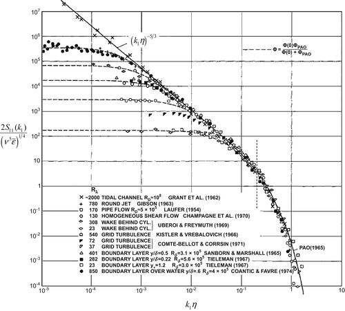
 is the average kinetic energy dissipation rate determined from (12.43). Kolmogorov's –5/3 power law is indicated by the sloping line. The collapse of the various spectra to this line and to each other as k1η approaches and then exceeds unity strongly suggests that high-wave-number turbulent velocity fluctuations are universal when the Reynolds number is high enough. The dashed vertical line indicates the location where the spectral data are a factor of two below the –5/3 line established at lower wave numbers.
 , Uj,
, Uj,  ,
,  ,
,  ,
,  ,
,  ,
,  ) are either uniform in space or zero. Thus, all the terms in (12.47) that include spatial differentiation of these averages and moments are zero, leaving:
 from (12.42) or (12.47) using the given velocity field is tedious but straightforward: