In this section, the equations of motion for the mean state in a turbulent flow are derived. The contribution of turbulent fluctuations appears in these equations as a correlation of velocity-component fluctuations. A turbulent flow instantaneously satisfies the Navier-Stokes equations. However, it is virtually impossible to predict the flow in detail at high Reynolds numbers, as there is an enormous range of length scales to be resolved (see Example 12.2) at each instant in time. Perhaps more importantly, knowledge of all these details is typically not necessary. If a commercial aircraft must fly from Los Angeles, California to Sydney, Australia, and turbulent skin-friction fluctuations occur in a frequency range from a few Hz to more than 104 Hz, the economically important parameter is the average skin friction because the time of the flight (many hours) is much longer than the even the longest fluctuation time scale. Here, the integrated effect of the fluctuations approaches zero when compared to the integral of the average. This situation where the overall duration of the flow far exceeds turbulent-fluctuation time scales is very common in engineering and geophysical science.
The following development of the mean-flow equations is for incompressible turbulent flow with constant viscosity where density fluctuations are caused by temperature fluctuations alone. The first step is to separate the dependent-field quantities into components representing the mean (capital letters and those with over bars) and those representing the deviation from the mean (lower case letters and those with primes):
u˜i=Ui+ui,p˜=P+p,ρ˜=ρ¯+ρ′,andT˜=T¯+T′
(12.24)
where – as in the preceding chapter – the complete field quantities are denoted by a tilde (∼). As mentioned in Section 12.3, this separation into mean and fluctuating components is called the Reynolds decomposition. Although it doubles the number of dependent field variables, this decomposition remains useful and relevant more than a century after it was first proposed. However, it leads to a closure problem in the resulting equation set that has still not been resolved without empiricism and modeling. The mean quantities in (12.24) are regarded as expected values,
u˜i¯=Ui,p˜¯=P,ρ˜¯=ρ¯,andT˜¯=T¯,
(12.25)
and the fluctuations have zero mean,
u¯i=0,p¯=0,ρ′¯=0,andT′¯=0.
(12.26)
The equations satisfied by the mean flow are obtained by substituting (12.24) into the governing equations and averaging. Here, the starting point is the Boussinesq set:
where the first equality in (4.86) and (4.89) follows from adding u˜i(∂u˜j/∂xj)=0 and T˜(∂u˜j/∂xj)=0, respectively, to the left-most sides of these equations. Simplifications for constant-density flow are readily obtained at the end of this equation-generation effort.
The continuity equation for the mean flow is obtained by putting the velocity decomposition of (12.24) into (4.10) and averaging:
The averages of each term in this equation can be determined by using (12.26) and the properties of an ensemble average: (12.4) through (12.6) and (12.8). The term-by-term results are:
This equation can be mildly rearranged using the final result of (12.27) and combining the gradient terms together to form the mean stress tensor τ¯ij:
where S¯ij=12(∂Ui/∂xj+∂Uj/∂xi) is the mean strain-rate tensor, and (4.40) has been used to put the mean viscous stress in the form shown in (12.30). The correlation tensor uiuj¯ in (12.30) is generally non-zero even though u¯i=0. Its presence in (12.30) is important because it has no counterpart in the instantaneous momentum equation (4.86) and it links the character of the fluctuations to the mean flow. Unfortunately, the process of reaching (12.30) does not provide any new equations for this correlation tensor. Thus, the final equality of (12.27), and (12.30) do not comprise a closed system of equations, even when the flow is isothermal.
The new tensor in (12.30), –ρ0uiuj¯, plays the role of a stress and is called the Reynolds stress tensor. When present, Reynolds stresses are often much larger than viscous stresses, μ(∂Ui/∂xj + ∂Uj/∂xi), except very close to a solid surface where the fluctuations go to zero and mean-flow gradients are large. The Reynolds stress tensor is symmetric since uiuj¯=ujui¯, so it has six independent Cartesian components. Its diagonal components u12¯, u22¯, and u32¯ are normal stresses that augment the mean pressure, while its off-diagonal components u1u2¯, u1u3¯, and u2u3¯ are shear stresses.
An explanation why the average product of the velocity fluctuations in a turbulent flow is not expected to be zero follows. Consider a shear flow where the mean shear dU/dy is positive (Figure 12.6). Assume that a fluid particle at level y travels upward because of a fluctuation (v > 0). On average this particle retains its original horizontal velocity during the migration, so when it arrives at level y + dy it finds itself in a region where a larger horizontal velocity prevails. Thus the particle is on average slower (u < 0) than neighboring fluid particles after it has reached the level y + dy. Conversely, fluid particles that travel downward (v < 0) tend to cause a positive u at their new level y−dy. Taken together, a positive v is associated with a negative u, and a negative v is associated with a positive u. Therefore, the correlation uv¯ is negative for the velocity field shown in Figure 12.6, where dU/dy > 0. This makes sense, since in this case the x-momentum should tend to flow in the negative y-direction as the turbulence tends to diffuse the gradients and decrease dU/dy.
Reynolds stresses arise from the nonlinear advection term uj(∂ui/∂xj) of the momentum equation, and are the average stress exerted by turbulent fluctuations on the mean flow. Another way to interpret the Reynolds stress is that it is the rate of mean momentum transfer by turbulent fluctuations. Consider again the shear flow U(y) shown in Figure 12.6, where the instantaneous velocity is (U + u, v, w). The fluctuating velocity components constantly transport fluid particles, and associated momentum, across a plane AA normal to the y-direction. The instantaneous rate of mass transfer across a unit area is ρ0v, and consequently the instantaneous rate of x-momentum transfer is ρ0(U + u)v. Per unit area, the average rate of flow of x-momentum in the y-direction is therefore
Figure 12.6 A schematic illustration of the development of non-zero Reynolds shear stress in a simple shear flow. A fluid particle that starts at y and is displaced upward to y + dy by a positive vertical velocity fluctuation v brings an average horizontal fluid velocity of U(y) that is lower than U(y + dy). Thus, a positive vertical velocity fluctuation v is correlated with negative horizontal velocity fluctuation u, so uv¯<0. Similarly, a negative v displaces the fluid particle to y – dy where it arrives on average with positive u, so again uv¯<0. Thus, turbulent fluctuations in shear flow are likely to produce negative non-zero Reynolds shear stress.
ρ0(U+u)v¯=ρ0Uu¯+ρ0uv¯=ρ0uv¯.
Generalizing, ρ0uiuj¯ is the average flux of i-momentum along the j-direction, which also equals the average flux of j-momentum along the i-direction.
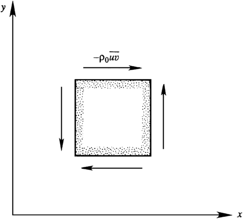
The sign convention for the Reynolds stress is the same as that explained in Section 2.4. On a surface whose outward normal points in the positive i-direction, a positive τij points along the j-direction. According to this convention, the Reynolds shear stresses –ρ0uiuj¯ (i ≠ j) on a rectangular element are directed as in Figure 12.7, if they are positive. Such a Reynolds stress causes mean transport of x-momentum along the negative y-direction.
The mean-flow thermal energy equation comes from substituting the velocity and temperature decompositions of (12.24) into (4.89) and averaging. The substitution step produces:
where k = ρocpκ is the thermal conductivity. Equation (12.32) shows that the fluctuations cause an additional mean turbulent heat flux ofρ0cpujT′¯ that has no equivalent in (4.89). The turbulent heat flux is the thermal equivalent of the Reynolds stress –ρ0uiuj¯ found in (12.30). Unfortunately, the process of reaching (12.31) and (12.32) has not provided any new equations for the turbulent heat flux. However, some understanding of the turbulent heat flux can be gained by considering diurnal heating of the earth's surface. During daylight hours, the sun may heat the surface of the earth, resulting in a mean temperature that decreases with height and in the potential for turbulent convective air motion. When such motions occur, an upward velocity fluctuation is mostly associated with a positive temperature fluctuation, giving rise to an upward heat flux ρ0cpu3T′¯>0.
The final mean-flow equation commonly considered for turbulent flows is that for transport of a dye or a non-reacting molecular species that is merely carried by the turbulent flow without altering the flow. Such passive contaminants are commonly called passive scalars or conserved scalars and the rate at which they are mixed with non-turbulent fluid is often of significant technological interest for pollutant dispersion and premixed combustion. Consider a simple binary mixture composed of a primary fluid with density ρ and a contaminant fluid (the passive scalar) with density ρs. The density ρm that results from mixing these two fluids is ρm=υ˜ρs+(1−υ˜)ρ, where υ˜ is the volume fraction of the passive scalar. The relevant conservation equation for the passive scalar is:
∂∂t(ρmY˜)+∂∂xj(ρmY˜u˜j)=∂∂xj(ρmκm∂∂xjY˜),
(12.33)
(see Kuo, 1986) where u˜j is the instantaneous mass-averaged velocity of the mixture, Y˜ is the mass fraction of the passive scalar, and κm is the mass-based molecular diffusivity of the passive scalar (see (1.1)). If the mean and fluctuating mass fraction of the conserved scalar are Y¯ and Y′, and the mixture density is constant, then the mean-flow passive scalar conservation equation is (see Exercise 12.12):
∂Y¯∂t+Uj∂Y¯∂xj=∂∂xj(κm∂Y¯∂xj−ujY′¯),
(12.34)
where ujY′¯ is the turbulent flux of the passive scalar. This equation is valid when the mixture density is constant, and this occurs when ρ = ρs = constant and when the contaminant is dilute so that ρm ≈ ρ = constant. If the amount of a passive scalar is characterized by a concentration (mass per unit volume), molecular number density, or mole fraction – instead of a mass fraction – the forms of (12.33) and (12.34) are unchanged but the diffusivity may need to be adjusted and molecular number or mass density factors may appear (see Bird et al. 1960; Kuo 1986). Equation (12.34) is of the same form as (12.32), and temperature may be considered a passive scalar in turbulent flows when it does not induce buoyancy, cause chemical reactions, or lead to significant density changes.
To summarize, (12.27), (12.30), (12.32), and (12.34) are the mean-flow equations for incompressible turbulent flow (in the Boussinesq approximation). The process of reaching these equations is known as Reynolds averaging, and it may be applied to the full compressible-flow equations of fluid motion as well. The equations that result from Reynolds averaging of any form of the Navier-Stokes equations are commonly known as RANS equations. The constant-density mean-flow RANS equations commonly used in hydrodynamics are obtained from the results provided in this section by dropping the gravity term and the “0” from ρ0 in (12.30), and reinterpreting the mean pressure as the deviation from hydrostatic (as explained in Section 4.9, “Neglect of Gravity in Constant Density Flows”).
The primary problem with RANS equations is that there are more unknowns than equations. The system of equations for the first moments depends on correlations involving pairs of variables (second moments). And, RANS equations developed for these pair correlations involve triple correlations. For example, the conservation equation for the Reynolds stress correlation, uiuj¯, is:
(see Exercise 12.16), and triple correlations appear in the third term on the left. Similar conservation equations for the triple correlations involve quadruple correlations, and the equations for the quadruple correlations depend on fifth-order correlations, and so on. This problem persists at all correlation levels and is known as the closure problem in turbulence. At the present time there are three approaches to the closure problem. The first, known as RANS closure modeling (see Section 12.10), involves terminating the equation hierarchy at a given level and closing the resulting system of equations with model equations developed from dimensional analysis, intuition, symmetry requirements, and experimental results. The second, known as direct numerical simulations (DNS) involves numerically solving the time-dependent equations of motion and then Reynolds averaging the computational output to determine mean-flow quantities. The third, known as large-eddy simulation (LES), combines elements of the other two and involves some modeling and some numerical simulation of large-scale turbulent fluctuations.
A secondary problem associated with the RANS equations is that the presence of the Reynolds stresses in (12.30) excludes the possibility of converting (12.30) into a Bernoulli equation, even when the density is constant and the terms containing ∂/∂t and ν are zero.
Example 12.5
Assume steady constant-density two-dimensional mean flow, and use (12.27) and (12.30) to redo the control volume analysis of Example 4.1 shown in Figure 4.2 to reach an integral formula for the average drag force F¯D on a two-dimensional body with span l in terms of the mean stream-wise velocity U and the normal Reynolds stress components in body's turbulent wake.
Solution
Here the analysis is similar to that in Example 4.1 with slightly different equations and integrands. To take advantage of the averaging in (12.27) and (12.30), their control volume form must be regenerated. For steady constant-density mean flow, (12.27) and (12.30) reduce to:
∂Uj∂xj=0andUj∂Ui∂xj=+1ρ∂∂xj(τ¯ij),
where τ¯ij is defined by the second equality of (12.30). Multiply the first of these with Ui and combine the result with the left side of the second equation to reach:
Now integrate the final equation within the control volume for Example 4.1 and use Gauss' divergence theorem to reduce to volume integral to an integral over its surface. Here, as in Example 4.1, the two vertical surfaces parallel to the flow upstream of the object each contribute half of the average drag force, F¯D. For conservation of horizontal momentum these steps lead to:
where “1” indicates the horizontal stream-wise direction. The equivalent conservation of mass statement is obtained from (12.27) by again using Gauss' divergence theorem and noting that the average mass flux is zero on the two vertical surfaces parallel to the flow upstream of the object.
(∫inlet+∫top+∫bottom+∫outlet)UjnjdA=0.
To reach the desired formula, choose “2” as the vertical direction, denote U1 = U and U2 = V, and subtract ∫P∞ndA = 0 from the momentum equation, where P∞ (= constant) is the pressure outside the turbulent wake far from the body. For two-dimensional mean flow, U3 = 0 so conservation of mass and horizontal momentum for the control volume of Example 4.1 imply:
where l is the width of the control volume transverse to the flow, U∞ is the steady horizontal flow speed upstream of the object, and u2¯ is the first normal Reynolds stress. Here the viscous and Reynolds stresses are only non-zero on the control volume's outlet surface, and the pressure on the inlet, top, and bottom of the control volume is P∞. To eliminate the integrals over the inlet, top, and bottom surfaces, multiply the conservation-of-mass equation by –ρU∞ and add it to the horizontal momentum equation to find:
F¯D=∫−H/2+H/2ρ(U∞U−U2+(P∞−P)+2νS11−u2¯)ldy.
Here, the remaining integral is over the outlet surface and H is the vertical height of the control volume.
Compared to the result of Example 4.1, this relationship for F¯D contains three extra terms. The final extra term is the turbulent normal stress from stream-wise velocity fluctuations and must be retained. The second extra term is the viscous normal stress and may be neglected compared to the final term when the flow is turbulent; the viscous stress was ignored in Example 4.1 as well. The first extra term involves the pressure difference, and represents the contribution of the second normal Reynolds stress when the mean flow is nearly parallel and the boundary-layer approximation applies. Consider the vertical component of (12.30) for constant density flow written in terms of (x,y)-coordinates:
U∂V∂x+V∂V∂y=−1ρ∂P∂y−∂∂xuv¯−∂∂yv2¯,
where again the viscous stresses have been ignored and v is the vertical velocity fluctuation. For nearly parallel flow in the horizontal direction (V ≪ U and ∂/∂x ≪ ∂/∂y), the boundary-layer approximation of this equation is:
0+0≅−1ρ∂P∂y−0−∂∂yv2¯or0≅∂∂y(P+ρv2¯),
which can be integrated and evaluated far from the turbulent wake where v = 0 and P = P∞ to find: P∞≅P+ρv2¯. Substituting this into the integral relationship for the drag force produces:
F¯Dρl≅∫−H/2+H/2(U(U∞−U)+v2¯−u2¯)dy,
which implies that the result of Example 4.1 is acceptable when the first and second normal Reynolds stresses are small or equal.
 (12.24)
 (12.25)
 (12.26)
 (4.10, 4.86)
 (4.89)
 and
and  , respectively, to the left-most sides of these equations. Simplifications for constant-density flow are readily obtained at the end of this equation-generation effort.
 (12.27)

 (12.28)
 (12.29)

 :
: (12.30)
 is the mean strain-rate tensor, and (4.40) has been used to put the mean viscous stress in the form shown in (12.30). The correlation tensor
  in (12.30) is generally non-zero even though
  . Its presence in (12.30) is important because it has no counterpart in the instantaneous momentum equation (4.86) and it links the character of the fluctuations to the mean flow. Unfortunately, the process of reaching (12.30) does not provide any new equations for this correlation tensor. Thus, the final equality of (12.27), and (12.30) do not comprise a closed system of equations, even when the flow is isothermal.
 , plays the role of a stress and is called the Reynolds stress tensor. When present, Reynolds stresses are often much larger than viscous stresses, μ(∂Ui/∂xj + ∂Uj/∂xi), except very close to a solid surface where the fluctuations go to zero and mean-flow gradients are large. The Reynolds stress tensor is symmetric since
  , so it has six independent Cartesian components. Its diagonal components
  ,
,  , and
, and  are normal stresses that augment the mean pressure, while its off-diagonal components
  ,
,  , and
, and  are shear stresses.
 is negative for the velocity field shown in Figure 12.6, where dU/dy > 0. This makes sense, since in this case the x-momentum should tend to flow in the negative y-direction as the turbulence tends to diffuse the gradients and decrease dU/dy.
 of the momentum equation, and are the average stress exerted by turbulent fluctuations on the mean flow. Another way to interpret the Reynolds stress is that it is the rate of mean momentum transfer by turbulent fluctuations. Consider again the shear flow U(y) shown in Figure 12.6, where the instantaneous velocity is (U + u, v, w). The fluctuating velocity components constantly transport fluid particles, and associated momentum, across a plane AA normal to the y-direction. The instantaneous rate of mass transfer across a unit area is ρ0v, and consequently the instantaneous rate of x-momentum transfer is ρ0(U + u)v. Per unit area, the average rate of flow of x-momentum in the y-direction is therefore
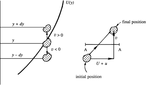
 . Similarly, a negative v displaces the fluid particle to y – dy where it arrives on average with positive u, so again
  . Thus, turbulent fluctuations in shear flow are likely to produce negative non-zero Reynolds shear stress.
 is the average flux of i-momentum along the j-direction, which also equals the average flux of j-momentum along the i-direction.
 (i ≠ j) on a rectangular element are directed as in Figure 12.7, if they are positive. Such a Reynolds stress causes mean transport of x-momentum along the negative y-direction.
 (12.31)
 (12.32)
 that has no equivalent in (4.89). The turbulent heat flux is the thermal equivalent of the Reynolds stress –ρ0
 found in (12.30). Unfortunately, the process of reaching (12.31) and (12.32) has not provided any new equations for the turbulent heat flux. However, some understanding of the turbulent heat flux can be gained by considering diurnal heating of the earth's surface. During daylight hours, the sun may heat the surface of the earth, resulting in a mean temperature that decreases with height and in the potential for turbulent convective air motion. When such motions occur, an upward velocity fluctuation is mostly associated with a positive temperature fluctuation, giving rise to an upward heat flux
  .
. , where
  is the volume fraction of the passive scalar. The relevant conservation equation for the passive scalar is:
 (12.33)
 is the instantaneous mass-averaged velocity of the mixture,
  is the mass fraction of the passive scalar, and κm is the mass-based molecular diffusivity of the passive scalar (see (1.1)). If the mean and fluctuating mass fraction of the conserved scalar are
  and Y′, and the mixture density is constant, then the mean-flow passive scalar conservation equation is (see Exercise 12.12):
 (12.34)
 is the turbulent flux of the passive scalar. This equation is valid when the mixture density is constant, and this occurs when ρ = ρs = constant and when the contaminant is dilute so that ρm ≈ ρ = constant. If the amount of a passive scalar is characterized by a concentration (mass per unit volume), molecular number density, or mole fraction – instead of a mass fraction – the forms of (12.33) and (12.34) are unchanged but the diffusivity may need to be adjusted and molecular number or mass density factors may appear (see Bird et al. 1960; Kuo 1986). Equation (12.34) is of the same form as (12.32), and temperature may be considered a passive scalar in turbulent flows when it does not induce buoyancy, cause chemical reactions, or lead to significant density changes.
 , is:
, is: (12.35)
 on a two-dimensional body with span l in terms of the mean stream-wise velocity U and the normal Reynolds stress components in body's turbulent wake.
 is defined by the second equality of (12.30). Multiply the first of these with Ui and combine the result with the left side of the second equation to reach:
 . For conservation of horizontal momentum these steps lead to:
 is the first normal Reynolds stress. Here the viscous and Reynolds stresses are only non-zero on the control volume's outlet surface, and the pressure on the inlet, top, and bottom of the control volume is P∞. To eliminate the integrals over the inlet, top, and bottom surfaces, multiply the conservation-of-mass equation by –ρU∞ and add it to the horizontal momentum equation to find:
 contains three extra terms. The final extra term is the turbulent normal stress from stream-wise velocity fluctuations and must be retained. The second extra term is the viscous normal stress and may be neglected compared to the final term when the flow is turbulent; the viscous stress was ignored in Example 4.1 as well. The first extra term involves the pressure difference, and represents the contribution of the second normal Reynolds stress when the mean flow is nearly parallel and the boundary-layer approximation applies. Consider the vertical component of (12.30) for constant density flow written in terms of (x,y)-coordinates:
 . Substituting this into the integral relationship for the drag force produces: