12.9. Wall-Bounded Turbulent Shear Flows

At sufficiently high Reynolds number, the characteristics of free turbulent shear flows discussed in the preceding section are independent of Reynolds number and may be self-similar based on a single length scale. However, neither of these simplifications occurs when the flow is bounded by one or more solid surfaces. The effects of viscosity are always felt near the wall where turbulent fluctuations go to zero, and this gives rise to a second fundamental length scale l_ν that complements the turbulent layer thickness δ. In addition, the persistent effects of viscosity are reflected in the fact that the skin-friction coefficient for a smooth flat plate or smooth round pipe depends on Re, even when Re → ∞, as seen in Figure 10.12. Therefore, Re independence of the flow as Re → ∞ does not occur in wall-bounded turbulent shear flows when the wall(s) is(are) smooth.

The importance of wall-bounded turbulence in engineering applications and geophysical situations is hard to overstate since it sets fundamental limits for the efficiency of transportation systems and on the exchange of mass, momentum, and heat at the earth's surface. Thus, the literature on wall-bounded turbulent flows is large and the material provided here merely covers the fundamentals of the mean flow. A more extensive presentation that includes turbulence intensities is provided in Chapter 7 of Pope (2000). Vortical structures in wall-bounded turbulence are discussed in Kline et al. (1967), Cantwell (1981), and Adrian (2007). The review articles by George (2006), Marusic et al. (2010), and Smits et al. (2011) are also recommended.

Three generic wall-bounded turbulent shear flows are described in this section: pressure-driven channel flow between stationary parallel plates, pressure-driven flow through a round pipe, and the turbulent boundary-layer flow that develops from nominally uniform flow over a flat plate. The first two are fully confined while the boundary layer has one free edge. The main differences between turbulent and laminar wall-bounded flows are illustrated on Figure 12.17. In general, mean turbulent-flow profiles (solid curves) are blunter, and turbulent-flow wall-shear stresses are higher than those of equivalent steady laminar flows (dashed curves). In addition, a turbulent boundary-layer, mean-velocity profile approaches the free-stream speed very gradually with increasing y so the full thickness of the profile shown in the right panel of Figure 12.17 lies beyond the extent of the figure. Throughout this section, the density of the flow is taken to be constant.

Fully developed channel flow is perhaps the simplest wall-bounded turbulent flow. Here, the modifier fully developed implies that the statistics of the flow are independent of the downstream direction. The analysis provided here is readily extended to pipe flow, after a suitable redefinition of coordinates. Further extension of channel flow results to boundary-layer flows is not as direct, but can be made when the boundary-layer approximation replaces the fully developed flow assumption. If we align the x-axis with the flow direction, and chose the y-axis in the cross-stream direction perpendicular to the plates so that y = 0 and y = h define the plate surfaces, then fully developed channel flow must have ∂U/∂x = 0. Hence, U can only depend on y, and it is the only mean-velocity component because the remainder of (12.27) implies ∂V/∂y = 0, and the boundary conditions V = 0 on y = 0 and h, then require V = 0 throughout the channel. Under these circumstances, the mean-flow momentum equations are:

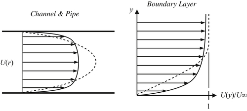
Figure 12.17 Sample profiles for wall-bounded turbulent flows (solid curves) compared to equivalent laminar profiles (dashed curves). In general turbulent profiles are blunter with higher skin friction; that is, μ(dU/dy) evaluated at the wall is greater in turbulent flows than in equivalent laminar ones. In channel and pipe flows, the steady laminar profile is parabolic while a mean turbulent flow profile is more uniform across the central 80% of the channel or pipe. For boundary layers having the same displacement thickness, the steady laminar profile remains linear farther above the wall and converges to the free-stream speed more rapidly than the mean turbulent profile.

0=−∂P∂x+∂τ¯∂yand0=−∂∂y(P+ρv2¯),

(12.76)

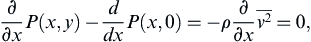
where τ¯=μ(∂U/∂y)−ρuv¯ is the total average stress and it cannot depend on x. Integrating the second of these equations from the lower wall up to y produces:

P(x,y)−P(x,0)=−ρv2¯+ρ[v2¯]y=0=−ρv2¯,

where the final equality follows because the variance of the vertical velocity fluctuation is zero at the wall (y = 0). Differentiating this with respect to x produces:

∂∂xP(x,y)−ddxP(x,0)=−ρ∂∂xv2¯=0,

(12.77)

where P(x,0) is the ensemble-average pressure on y = 0 and the final equality follows from the fully developed flow assumption. Thus, the stream-wise pressure gradient is only a function of x; ∂P(x,y)/∂x = dP(x,0)/dx. Therefore, the only way for the first equation of (12.76) to be valid is for ∂P/∂x and ∂τ¯/∂y to each be constant, so the total average stress distribution τ¯(y) in turbulent channel flow is linear as shown in Figure 12.18a. Away from the wall, τ¯ is due mostly to the Reynolds stress, close to the wall the viscous contribution dominates, and at the wall the stress is entirely viscous.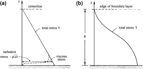

Figure 12.18 Variation of total shear stress across a turbulent channel flow (a) and through a zero-pressure-gradient turbulent boundary layer (b). In both cases, the Reynolds shear stress dominates away from the wall but the viscous shear stress takes over close to the wall. The shape of the two stress curves is set by momentum transport between the fast-moving part of the flow and the wall where U = 0.

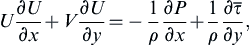
For a boundary layer on a flat plate, the stream-wise mean-flow momentum equation is:

U∂U∂x+V∂U∂y=−1ρ∂P∂x+1ρ∂τ¯∂y,

(12.78)

where τ¯ is a function of x and y. The variation of the stress across a boundary layer is sketched in Figure 12.18b for the zero-pressure-gradient (ZPG) condition. Here, a constant stress layer, ∂τ¯/∂y ≈ 0, occurs near the wall since both U and V → 0 as y → 0. When the pressure gradient is not zero, the stress profile approaches the wall with a constant slope. Although it is not shown in the figure, the structure of the near-wall region of the turbulent boundary layer is similar to that depicted for the channel flow in Figure 12.18a with viscous stresses dominating at and near the wall.

The partitioning of the stress based on its viscous and turbulent origins leads to the identification of two different scaling laws for wall-bounded turbulent flows. The first is known as the law of the wall and it applies throughout the region of the boundary layer where viscosity matters and the largest relevant length scale is y, the distance from the wall. This region of the flow is typically called the inner layer. The second scaling law is known as the velocity defect law, and it applies where the flow is largely independent of viscosity and the largest relevant length scale is the overall thickness of the turbulent layer δ. This region of the flow is typically called the outer layer. Fortunately, the inner and outer layers of wall-bounded turbulent flow overlap, and in this overlap region the form of the mean stream-wise velocity profile may be deduced from dimensional analysis.

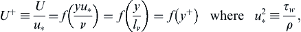
Inner Layer: Law of the Wall

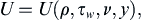
Consider the flow near the wall of a channel, pipe, or boundary layer. Let U_∞ be the centerline velocity in the channel or pipe, or the free-stream velocity outside the boundary layer. Let δ be the thickness of the flow between the wall and the location where U = U_∞. Thus, δ may be the channel half width, the radius of the pipe, or the boundary-layer thickness. Assume that the wall is smooth, so that any surface roughness is too small to affect the flow. Physical considerations suggest that the near-wall velocity profile should depend only on the near-wall parameters and not on U_∞ or the thickness of the flow δ. Thus, very near the smooth surface, we expect:

U=U(ρ,τw,ν,y),

(12.79)

where τ_w is the shear stress on the smooth surface. This equation may be recast in dimensionless form as:

U+≡Uu∗=f(yu∗ν)=f(ylν)=f(y+)whereu∗2≡τwρ,

(12.80, 12.81)

f is an undetermined function, u_∗ is the friction velocity or shear velocity, and l_ν = ν/u_∗ is the viscous wall unit. Equation (12.80) is the law of the wall and it states that U/u_∗ should be a universal function of yu_∗/ν near a smooth wall. The superscript plus signs are standard notation for indicating a dimensionless law-of-the-wall variable.

The inner part of the wall layer, right next to the wall, is dominated by viscous effects and is called the viscous sub-layer. In spite of the fact that it contains fluctuations, the Reynolds stresses are small here because the presence of the wall quells wall-normal velocity fluctuations. At high Reynolds numbers, the viscous sub-layer is thin enough so that the stress is uniform within the layer and equal to the wall shear stress τ_w. Therefore the mean-velocity gradient in the viscous sub-layer is given by:

μ(dU/dy)=τw→U=τwy/μorU+=y+,

(12.82)

where the second two equalities follow from integrating the first. Equation (12.82) shows that the velocity distribution is linear in the viscous sub-layer, and experiments confirm that this linearity holds up to yu_∗/ν ≈ 5, which may be taken to be the limit of the viscous sub-layer.

Outer Layer: Velocity Defect Law

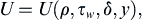
Now consider the velocity distribution in the outer part of a turbulent boundary layer. The gross characteristics of the turbulence in the outer region are inviscid and resemble those of a free shear flow. The existence of Reynolds stresses in the outer region results in a drag on the flow and generates a velocity defect ΔU = U_∞ − U, just like the planar wake. Therefore, in the outer layer we expect,

U=U(ρ,τw,δ,y),

(12.83)

and by dimensional analysis can write:

U∞−Uu∗=F(yδ)=F(ξ)

(12.84)

so that the defect velocity, U_∞ – U, is proportional to the friction velocity u_∗ and a profile function. This is called the velocity defect law, and this is its traditional form. In the last two decades, it has been the topic of considerable discussion in the research community, and alternative velocity and length scales have been proposed for use in (12.84), especially for turbulent boundary-layer flows.

Overlap Layer: Logarithmic Law

From the preceding discussion, the mean-velocity profiles in the inner and outer layers of a wall-bounded turbulent flow are governed by different laws, (12.80) and (12.84), in which the independent coordinate y is scaled differently. Distances in the outer part are scaled by δ, whereas those in the inner part are scaled by the much smaller viscous wall unit l_ν = ν/u_∗. Thus, wall-bounded turbulent flows involve at least two turbulent length scales, and this prevents them from reaching the same type of self-similar form with increasing Reynolds number as that found for simple free turbulent shear flows.

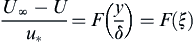
Interestingly, a region of overlap in the two profile forms can be found by taking the limits y⁺ → ∞ and ξ → 0 simultaneously. Instead of matching the mean velocity directly, in this case it is more convenient to match mean-velocity gradients. (The following short derivation closely follows that in Tennekes and Lumley, 1972.) From (12.80) and (12.84), dU/dy in the inner and outer regions is given by:

dUdy=u∗2νdfdy+and−dUdy=u∗δdFdξ,

(12.85, 12.86)

respectively. Equating these and multiplying by y/u_∗, produces:

−ξdFdξ=y+dfdy+,

(12.87)

an equation that should be valid for large y₊ and small ξ. As the left-hand side can only be a function of ξ and the right-hand side can only be a function of y⁺, both sides must be equal to the same universal constant, say 1/κ, where κ is the von Karman constant (not the thermal diffusivity). Experiments show that κ ≈ 0.4 with some dependence on flow type and pressure gradient, as is discussed further on in this section. Setting each side of (12.87) equal to 1/κ, integrating, and using (12.80) gives:

U+≡Uu∗=f(y+)=1κln(y+)+BandF(ξ)=−1κln(ξ)+A,

(12.88, 12.89)

where B and A are constants with values around 4 or 5, and 1, respectively, again with some dependence on flow type and pressure gradient. Equation (12.88) or (12.89) is the mean-velocity profile in the overlap layer or the logarithmic layer. In addition, the constants in (12.88), κ and B, are known as the logarithmic-law (or log-law) constants. As the derivation shows, (12.88) and (12.89) are only valid for large y⁺ and small y/δ, respectively. The foregoing method of justifying the logarithmic velocity distribution near a wall was first given by Clark B. Millikan in 1938. The logarithmic law, however, was known from experiments conducted by the German researchers, and several derivations based on semi-empirical theories were proposed by Prandtl and von Karman. One such derivation using the so-called mixing length theory is presented in the following section.

The logarithmic law (12.88) may be the best-known and most important result for wall-bounded turbulent flows. Experimental confirmation of this law is shown in Figures 12.19 and 12.20 in law-of-the-wall and velocity-defect coordinates, respectively, for the turbulent boundary-layer data reported in Oweis et al. (2010) and Winkel et al. (2012). Nominal specifications for the extent of the viscous sub-layer, the buffer layer, the logarithmic layer, and the wake region are shown there as well. On Figure 12.19, the linear viscous sub-layer profile appears as a curve for y⁺ < 5. However, a logarithmic velocity profile appears as a straight line on a log-linear plot, and such a linear region is evident for approximately two decades in y⁺ starting near y⁺ ∼ 10². The extent of this logarithmic region increases in these coordinates with increasing Reynolds number. The region 5 < y⁺ < 30, where the velocity distribution is neither linear nor logarithmic, is called the buffer layer. Neither the viscous stress nor the Reynolds stresses are negligible here, and this layer is dynamically important because turbulence production reaches a maximum here. For the data shown, the measured profiles collapse well to a single curve below y⁺ ∼ 10⁴ (or y/δ ∼ 0.2) in conformance with the law of the wall. For larger values of y⁺, this profile collapse ends where the overlap region ends and the boundary layer's wake flow begins. These velocity profiles do not collapse in the wake region when plotted with law-of-the-wall normalizations because the wake-flow similarity variable is y/δ (not y/l_ν) and the ratio δ⁺ = δ/l_ν (commonly known as Re_τ) is different at the three different Reynolds numbers. The fitted curves shown in Figure 12.19 are mildly adjusted versions of those recommended in Monkewitiz et al. (2007) for smooth-flat-plate ZPG turbulent boundary layers.

Although the wake region appears to be smaller than the log-region on Figure 12.19, this is an artifact of the logarithmic horizontal axis. A turbulent boundary layer's wake region typically occupies the outer 80% of the flow's full thickness and this is shown more clearly in Figure 12.20 where measured mean-flow profiles are plotted in the velocity deficit form of (12.84). Here, again, the collapse of the various profiles to a single curve is excellent, and the measured profiles diverge from the log-law near y/δ ∼ 0.2.

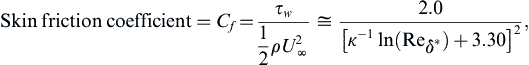
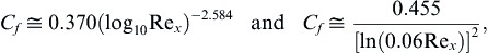
For fully developed channel and pipe flows, the mean stream-wise velocity profile does not evolve with increasing downstream distance. However, turbulent boundary layers do thicken. The following parameter results are developed from the systematic fitting and expansion efforts for ZPG turbulent boundary layers described in Monkewitz et al. (2007), and are intended for use when Re_x > 10⁶:

Momentumthickness=θ/x≈0.016Rex−0.15,

(12.90)

Displacementthickness=δ∗≈θexp{7.11κln(Reθ)},

(12.91)

99%thickness=δ99=0.2δ∗[κ−1ln(Reδ∗)+3.30],and

(12.92)

Skinfrictioncoefficient=Cf=τw12ρU∞2≅2.0[κ−1ln(Reδ∗)+3.30]2,

(12.93a)

where x is the downstream distance, Re_x = U_∞x/ν, Re_θ = U_∞θ/ν, and Re_δ∗ = U_∞δ∗/ν. Other common ZPG turbulent boundary-layer skin-friction correlations are those by Schultz-Grunow (1941) and White (2006):

Cf≅0.370(log10Rex)−2.584andCf≅0.455[ln(0.06Rex)]2,

(12.93b, 12.93c)

respectively. These formulae should be used cautiously because the influence of a boundary layer's virtual origin has not been explicitly included and it may be substantial (Chauhan et al., 2009; see also Marusic, 2010).

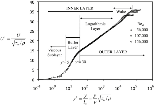
Figure 12.19 Mean-velocity profile of a smooth-flat-plate turbulent boundary layer plotted in log-linear coordinates with law-of-the-wall normalizations. The data are replotted from Oweis et al. (2010) and represent three Reynolds numbers. The extent of the various layers within a wall-bounded turbulent flow is indicated by vertical dashed lines. The log-layer-to-wake-region boundary is usually assumed to begin at y/δ ≈ 0.10 to 0.20 in turbulent boundary layers. Overall the data collapse well for the inner layer region, as expected, and the logarithmic layer extends for approximately two decades. The wake region shows differences between the Reynolds numbers because its similarity variable is y/δ, and δ/l_ν differs between the various Reynolds numbers.

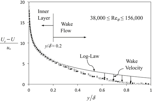
Figure 12.20 Mean-velocity profile of a smooth-flat-plate turbulent boundary layer plotted using the velocity defect coordinates of (12.84). The plotted data represent twelve different velocity profiles from the experiments reported in Oweis et al. (2010) and Winkel et al. (2012) covering the Reynolds number range 38,000 ≤ Re_θ≤ 156,000. Here, the log-law diverges from the measured profiles at y/δ ∼ 0.20. The measurement-log law difference represents the wake component of the mean-velocity profile. In these experiments, there was a slight favorable pressure gradient so the strength of the wake flow is about ∼25% lower than that in a zero-pressure-gradient boundary layer.

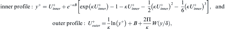
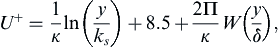
For the purpose of completeness, the following approximate mean-velocity profile functions are offered for wall-bounded turbulent flows:

innerprofile:y+=Uinner++e−κB[exp(κUinner+)−1−κUinner+−12(κUinner+)2−16(κUinner+)3],andouterprofile:Uouter+=1κln(y+)+B+2ΠκW(y/δ),

(12.94, 12.95)

where the inner profile from Spalding (1961) is specified in implicit form, κ and B are the log-law constants from (12.88), and Π and W are the wake strength parameter and a wake function, respectively, both introduced by Coles (1956). The wake function W and the length scale δ in its argument are empirical and are typically determined by fitting curves to experimental profile data.

Example 12.9

Estimate the boundary-layer thicknesses on the underside of the wing of a large commercial airliner on its landing approach. Use the flat-plate results provided above, a chord-length distance of x = 8m, a flow speed of 100 m/s, and a nominal value of κ ≈ 0.4.

Solution

First, compute the downstream-distance Reynolds number Re_x using the nominal kinematic viscosity of air: Re_x = (100m/s)(8m)/(1.5×10−5m2/s)=53×106. This Reynolds number is clearly high enough for turbulent flow, so the estimates are:

θ≈0.016·Rex−0.15·x=0.016(53×106)−0.15(8m)=0.0089m,

 

δ∗≈θexp{7.11κln(Reθ)}=(0.0089m)exp{7.11(0.4)ln((0.0089m)(100m/s)/1.5×10−5m2/s)}≅0.0115m,andδ99=0.2δ∗[κ−1ln(Reδ∗)+3.30]=0.2(0.0115m)[0.4−1ln((0.0115m)(100m/s)1.5×10−5m2/s)+3.30]≅0.072m.

 

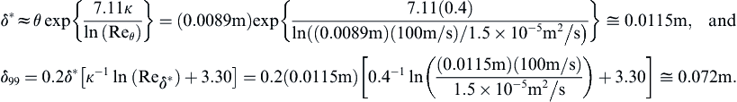
Here, we note that θ and δ∗ are almost an order of magnitude smaller than δ₉₉, and that all three boundary-layer thicknesses are miniscule compared to the wing's chord length of 8m. The latter finding is a primary reason why boundary-layer thicknesses are commonly ignored in aerodynamic analyses.

Of the three generic wall-bounded turbulent flows, the boundary layer's wake is typically the most prominent. For ZPG boundary layers the wake strength is Π = 0.44 (Chauhan et al., 2009). When the pressure gradient is favorable, Π is lower, and when the pressure gradient is adverse, Π is higher. The wake function is typically chosen to go smoothly from zero to unity as y goes from zero to δ. Among the simplest possibilities for W(ξ) are 3ξ² – 2ξ³ and sin²(πξ/2), however more sophisticated fits are currently in use (see Monkewitz et al., 2007; Chauhan et al., 2009). In the outer profile form given above, δ is interpreted as the 100% boundary-layer thickness where U first equals the local free-stream velocity as y increases. In practice, this requirement cannot be evaluated perfectly with finite-precision experimental data so δ is often approximated as being the 99% or the 99.5% thickness, δ₉₉ or δ_99.5, respectively. Of course, for channel or pipe flows, δ is half the channel height or the pipe radius, respectively.

As of this writing, new and important concepts and results for wall-bounded turbulence continue to emerge. These include the possibility that the overlap layer might instead be of power law form (Barenblatt, 1993; George & Castillo, 1997) and a reinterpretation of the layer structure in terms of stress gradients (Wei et al., 2005; Fife et al., 2005). The comparisons in Monkewitz et al. (2008) suggest that the logarithmic law should be favored over a power law, while the implications of the stress gradient balance approach are still under consideration. These and other topics in the current wall-bounded turbulent flow literature are discussed in Marusic et al. (2010) and Smits et al. (2011).

Perhaps the most fundamental unanswered question concerns the universality of wall-bounded turbulent flow profiles; are all wall-bounded turbulent flows universal (statistically the same) when scaled appropriately? To answer this question, consider the inner, outer, and overlap layers separately. First of all, the viscous sub-layer profile U⁺ = y⁺ (12.82) is universal using law-of-the-wall normalizations. However, geometrical differences suggest that the wake flow region is not universal. Consider the zone of maximum average fluid velocity at the outer edge of the wake portion of a wall-bounded flow. This maximum velocity zone occurs on the centerline of a channel flow (a plane), on the centerline of a pipe flow (a line), and at the edge of a boundary layer (a slightly tilted, nearly planar surface). Thus, the ratio of the maximum-velocity area to the bounding-wall surface area is one-half for channel flow, vanishingly small for pipe flow, and slightly greater than unity for boundary-layer flow. On this basis, the three wake flows are distinguished. Additionally, the boundary layer differs from the other two flows because it is bounded on one side only. The boundary layer's wake-flow region entrains irrotational fluid at its free edge and does not collide or interact with turbulence arising from an opposing wall, as is the case for channel and pipe flows. Thus, the wake-flow regions of these wall-bounded turbulent flows should all be different and not universal.

Now consider the overlap layer in which the mean-velocity profile takes a logarithmic form. Logarithmic profiles have been observed in all three generic wall-bounded turbulent flows, and Coles and Hirst (1968) recommended values of κ = 0.41 and B = 5.0 for the log-law constants. However, in each circumstance, the log layer inherits properties from the universal viscous sub-layer and from a non-universal wake flow. Thus, the log-law (12.88) may imperfectly approach universality, and this situation is found in experiments. In particular, an assessment of published literature (Nagib & Chauhan, 2008) supports the following values for the logarithmic-law constants at high Reynolds numbers:

Channelflow:κ=0.37B=3.7Pipeflow:κ=0.41B=5.0ZPGboundarylayer:κ=0.384B=4.17

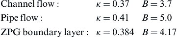
Yet, the situation remains unsettled. Recent channel-flow experiments at Re_h = U_avh/ν up to 300,000 (where h is the full channel height, and U_av is the time- and height-averaged flow speed) again find κ = 0.41 and B = 5.0 (Schultz & Flack, 2012). Plus, an assessment of the highest Reynolds number data available suggest that turbulent pipe and boundary-layer flows may share log-law constants (κ = 0.39 and B = 4.3) in the range 3u∗δ/ν<y+ and y < 0.15δ, where δ is the full boundary-layer thickness (Marusic et al., 2013).

The observed flow-to-flow variation in log-law constants is not anticipated by the analysis presented earlier in this section because geometric differences in the wake-flow regions were not accounted for in (12.83). However, the previous analysis remains valid for each outer-layer flow geometry. Thus, the log-law (12.88) does describe the overlap layer of wall-bounded turbulent flows when the log-law constants are appropriate for that flow's geometry.

Interestingly, there is another issue at play here for turbulent boundary layers. From a flow-parameter perspective, a turbulent boundary layer differs from fully developed channel and pipe flows because the pressure gradient that may exist in a boundary-layer flow is not directly linked to the wall shear stress τ_w. In fully developed channel and pipe flow, a stationary control volume calculation (see Exercise 12.34) requires:

dP/dx=−2τw/hordP/dx=−4τw/d,

(12.96, 12.97)

respectively, where h is the channel height and d is the pipe diameter. Thus, the starting points for the dimensional analysis of the inner and outer layers of the mean-velocity profile, (12.79) and (12.83), need not include dP/dx for pipe and channel flows because τ_w is already included. Yet, there is no equivalent to (12.96) or (12.97) for turbulent boundary layers. More general forms of (12.79) and (12.83) that would be applicable to all turbulent boundary layers need to include ∂P/∂x, especially since ∂P/∂x does not drop from the mean stream-wise momentum equation, (12.78), for any value of y when ∂P/∂x is non-zero. The apparent outcome of this situation is that the log-law constants in turbulent boundary layers depend on the pressure gradient. Surprisingly, the following empirical correlation, offered by Nagib and Chauhan (2008):

κB=1.6[exp(0.1663B)−1],

(12.98)

collapses measured values of κ and B from all three types of wall-bounded shear flows for 0.15 < κ < 0.80, and –4 < B < 12. Here, the most extreme values of κ and B arise from turbulent boundary layers in adverse (low values of κ and B) and favorable (high values of κ and B) pressure gradients.

Turbulent Flow in Ducts

Fully enclosed turbulent flows through tubes, pipes, ducts, and other conduits have historical, scientific, and practical importance. The study of wall-bounded turbulence originates in the pipe flow studies of Hagen, Poiseuille, Darcy, and Reynolds (see Mullin, 2011). Modern laboratory pipe flow experiments (Zagarola & Smits 1998, McKeon et al., 2004, Hultmark et al., 2012) have reached higher Reynolds numbers than equivalent studies of channel and boundary-layer flows, and thereby have been pivotal in developing a more nuanced understanding of wall-bounded turbulence. Plus, water, air, gasoline, natural gas, crude oil, and variety of other liquids and gases are commonly conveyed from place to place in the developed world through pipelines and other fully-enclosed conduits for economic, and health- and safety-related reasons.

A general understanding of duct flows can be developed by considering nominally-steady fully-developed constant-density flow in an straight fully-enclosed duct with smooth walls and constant cross-sectional area A. Consider a simple momentum balance for a duct segment of length L shown in Figure 12.21. Time-averaging the horizontal component of (4.17) with this duct segment as the control volume and with b = 0 when gravity is vertical leads to:

−∫Aρ(U2+u2¯)udA+∫Aρ(U2+u2¯)ddA=(Pu−Pd)A−L∫0lτwds,

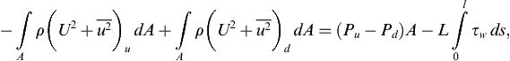(12.99)

where the u- and d-subscripts denote the upstream and downstream duct cross-sections, respectively, and the interior perimeter of the duct cross section has length l. For fully developed flow, the momentum flux terms on the left of (12.99) cancel, so the equation reduces to:

Pu−PdL=lA(1l∫0lτwds)=lAτ¯w,

(12.100)

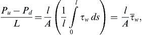
where τ¯w is the perimeter- and time-averaged wall shear stress. Thus, the pressure difference necessary to maintain the flow is directly proportional to τ¯w. Equation (12.100) is commonly recast in terms of the Darcy friction factor, f¯, by scaling the pressure difference with the duct length L and 12ρUav2:

Pu−Pd=12ρUav2·Ldh·f¯orf¯=4C¯f

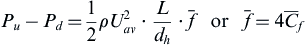(12.101, 12.102)

where Uav=(1/A)∫AreaUdA 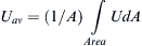is the time and cross-sectional-area averaged flow speed in the duct, C¯f=τ¯w/12ρUav2 is the average skin friction coefficient (or Fanning friction factor), and d_h is the hydraulic diameter of the duct:

dh=4A/l,

(12.103)

defined so that it reduces to pipe-interior diameter when the duct is round.

Figure 12.21 A segment L of a straight duct of non-circular but constant cross-sectional area A. The average momentum flux into and out of the duct will be equal so conservation of momentum within the duct reduces to a balance of the pressure force (P_u – P_d)A, and the integrated wall-shear stress L∫0lτwds acting on the fluid in the duct segment.

In this smooth-wall formulation, the friction factor, f¯, may depend on Reynolds number and duct geometry. Consider first the implications of the outer flow profile (12.91) and the simplified momentum balance (12.101) for round pipes where d_h = d = the geometrical pipe diameter. For turbulent flow, the viscous sub-layer is thin and the wake component in (12.101) is weak in round pipes. Thus, (12.88) may integrated throughout the cross-section of the pipe to find:

Uav≅u∗[(1/κ)ln(du∗/2ν)+B−3/2κ],

(12.104)

and this can be converted into an implicit relationship for the Darcy friction factor using the generic log-law constants κ = 0.41 and B = 5.0:

f¯−1/2≅2.0log10(Redf¯1/2)−1.0,

(12.105)

(see Exercise 12.37) to reach a formula first derived by Prandtl in 1935. To compensate for neglecting the viscous sub-layer and the wake contribution near the pipe's centerline, he modified the second constant:

f¯−1/2≅2.0log10(Redf¯1/2)−0.8.

(12.106)

to better match the available experimental data. This empirical formula is valid for Re_d ≥ 4000 (White, 2006) and yields f¯-values substantially larger than the laminar pipe flow result f¯=64/Red. Although some adjustments to the constants have been recommended (Zagarola & Smits 1998; McKeon et al., 2004), (12.106) still provides a worthwhile quantitative means for determining the Reynolds number dependence of f¯.

The dependence of f¯ on duct geometry is commonly managed for engineering purposes by using a non-circular conduit's hydraulic diameter in (12.106). The implicit assumption here is that τ¯w has the same relationship to U_av in non-circular ducts as it does in circular ones. However, this approach looses accuracy when the duct cross-section has sharp corners or when it has a high width-to-height aspect ratio because the conduit's Reynolds number based on hydraulic diameter, U_avd_h/ν, is too large. Such difficulties can be partially corrected in rectangular and annual ducts by adjusting the Reynolds number in (12.106) downward using laminar flow results:

f¯duct,turb−1/2≅2.0log10((f¯pipe·Redf¯duct·Redh)laminar·Redh·f¯duct,turb−1/2)−0.8

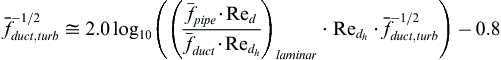(12.107)

(see Jones 1976, Jones and Leung 1981). The added laminar-flow factor in (12.107) may be obtained from tabulations of laminar flow results (see White 2006) and is 2/3 when the duct is a high-aspect-ratio channel. A review of flow friction in non-circular ducts and an alternative correction scheme for (12.106) are provided in Obot (1988).

Rough Surfaces

In deriving the logarithmic law (12.88), we assumed that the flow closest to the wall is determined by viscosity. This is true only for hydrodynamically smooth surfaces, for which the average height of the surface roughness elements is less than the thickness of the viscous sub-layer. For a hydrodynamically rough surface, on the other hand, the roughness elements are taller than the viscous sub-layer (if it exists), and may prevent its formation. An extreme example is the atmospheric boundary layer, where vegetation, buildings, etc., act as roughness elements. In such fully rough situations, the boundary-layer flow impinges directly on the roughness elements leading to wake formation behind each element. Here, shear stress is transmitted to the wall by the resulting drag on the roughness elements, and it nearly always exceeds equivalent smooth wall values. For such fully rough conditions, viscosity is irrelevant for determining either the velocity distribution or the overall friction drag on the surface. This is why the friction coefficients for rough-wall pipes become constant as Re → ∞.

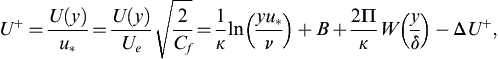
Although turbulent wall bounded flows over rough surfaces have been of interest for more than a century (Jimenez, 2004), a full understanding of such flows remains elusive and empirical correlations are commonly used for predicting the character of such flows (Flack & Schultz, 2010). The phenomenology of turbulent flow near a rough wall is depicted in Figures 12.22 and 12.23, which show mean stream-wise velocity profiles in physical and law-of-the-wall coordinates, respectively. When the surface is fully rough, the viscous sub-layer is lost and the velocity distribution above the roughness elements is logarithmic, but the log-law intercept constant is lower than the equivalent smooth-wall value. This downward shift in the log-law, ΔU⁺, is known as the roughness function (see Figure 12.23). Thus, rough-wall turbulent velocity profiles are adequately described by:

U+=U(y)u∗=U(y)Ue2Cf=1κln(yu∗ν)+B+2ΠκW(yδ)−ΔU+,

(12.108)

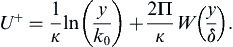
where ΔU⁺ provides the roughness correction to the smooth wall result (12.91). For pipes and channels, U_e is typically chosen equal to U_av, while for boundary layers it is the average wall-parallel velocity at the location y = δ. Similarly, C_f is the skin friction coefficient based on U_av or U_e, and δ is understood to be the channel half-height, pipe radius, or overall boundary-layer thicknesses, as appropriate for the flow's geometry. In geophysical flows, the first, second, and last terms on the right-most side of (12.108) are commonly combined and written in terms of a roughness height k₀ that is defined as the value of y at which the logarithmic velocity profile gives U = 0 (Figure 12.22b):

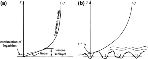
Figure 12.22 Logarithmic velocity distributions near smooth (a) and rough (b) surfaces. The presence of surface roughness may eliminate the viscous sub-layer when the roughness elements protrude higher than several l_ν. In this case the log-law may be extended to a virtual wall location y = k₀ where U appears to go to zero.

Figure 12.23 Average stream-wise velocity profiles, U⁺ =  U(y)/u_∗, near smooth (ΔU⁺ =  0) and rough (ΔU⁺ > 0) surfaces in law-of-the-wall coordinates where y is the wall normal distance, and y⁺ =  yu_∗/ν [see (12.80) and (12.81)]. When the wall is rough, the skin friction is higher and this causes the log-law portion of the velocity profile to shift downward by an amount ΔU⁺, known as the roughness function.

U+=1κln(yk0)+2ΠκW(yδ).

(12.109)

Here, k₀ carries the roughness correction, and the two formulations, (12.108) and (12.109), are equivalent. The wake portion of wall-bounded turbulent flows is consistently found to be unaltered by the presence of wall roughness (Flack & Schultz, 2010) even though roughness does tend to increase δ for boundary-layer flows.

This phenomenology introduces at least two conundrums. The first is the location of y = 0. In experimental work, this location is typically chosen to lie somewhere between the peaks and valleys of the roughness elements to maximize the quality of a logarithmic fit to the measured velocity profile. The second, and more important, is the quantitative connection between the actual spatial profile of the rough surface and the resulting surface friction for a given flow speed and flow geometry (channel, pipe, boundary layer, etc.). A rough surface may have structured (patterned) or random roughness, and, in general, must be characterized by multiple length scales such as average or root-mean-square roughness height (k or k_rms), and surface correlation lengths in the stream-wise and cross-stream directions. The first quantitative work on this topic was conducted by Nikuradse (1933) who studied the impact of uniform-size sand-grain roughness on pipe flow friction using average-sand-grain diameter to characterize the roughness height of the surface. His work has remained important and compelling so that essentially all subsequent rough-wall friction measurements have been reported in terms of equivalent sand-grain roughness height, k_s.

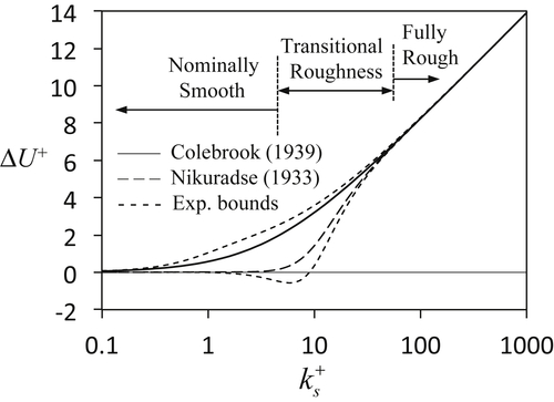
Figure 12.24 Roughness function, ΔU⁺, as a function of law-of-the-wall-scaled equivalent sand-grain roughness height, ks+=ksu∗/ν. The solid curve is the correlation of Colebrook (1939) for surfaces typical of commercial pipes. The long-dash curve follows the sand-grain roughness results of Nikuradse (1933). The short-dash curves provide approximate upper and lower bounds for experimental results from a variety of rough surfaces. Although the chosen normalizations produce consistent results below ks+ of unity and above ks+ of ∼50, this figure shows that k_s alone is insufficient to describe the effects of wall roughness in between these nominal limiting values.

Figure 12.24 shows how the roughness function ΔU⁺ depends on the law-of-the-wall-scaled equivalent sand-grain roughness height ks+=ksu∗/ν. The sand-grain results are indicated with long dashes, and are commonly used to define three regimes:

nominallysmooth:ks+<4,transitionallyrough:4<ks+<70,andfullyrough:70<ks+.

In the nominally smooth (also know as hydraulically smooth) regime, sand-grain roughness has no effect, but other types of wall roughness may still cause a roughness effect (Colebrook 1939). More recently, the measured onset of roughness effects has been found to occur at kt+ ∼ 9 (Flack et al., 2012), where k_t is the peak-to-trough roughness height. In the transitional roughness regime, the roughness function cannot be characterized by ks+ alone. Here, surfaces typical of commercial piping produce the higher values of ΔU⁺, while triangular riblets may even produce small negative values of ΔU⁺ corresponding to skin friction reduction (see Figure 3 and discussion in Jimenez (2004)). In the fully rough regime, the effects of roughness are independent of the Reynolds number, and ΔU⁺ depends logarithmically on ks+.

In 1939, Colebrook devised an interpolation formula for the Darcy friction factor for surface roughness typical of commercial piping that spans the three regimes:

f¯−1/2≅−2.0log10(ks/d3.7+2.51Redf¯1/2)

(12.110)

This interpolation formula reduces to (12.106) when k_s = 0, and it results in the well-known Moody diagram (Moody 1994) when f¯ is plotted vs. Re_d for different values of k_s/d. An alternative form of (12.110), provided in Jimenez (2004):

ΔU+=1κln(1+0.26ks+),

(12.111)

appears on Figure 12.24 as the solid curve. In (12.111) the value of κ is presumed to be 0.40, so that when (12.110) is substituted into (12.108), Nikuradse's fully-rough velocity profile:

U+=1κln(yks)+8.5+2ΠκW(yδ),

(12.112)

is recovered. As expected, this profile is independent of ν.

With Colebrook's interpolation formula, the flow friction associated with a rough surface can be estimated when that surface's equivalent sand-grain roughness is known. Traditionally, determination of equivalent sand grain roughness required experimental tests. However, Flack et al. (2010) have recently suggested that k_s can be determined from the root-mean-square roughness height k_rms, and the standardized skewness, s_k = (skewness)/krms3, of the surface elevation probability density function:

ks=4.43krms(1+sk)1.37.

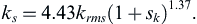(12.113)

Example 12.10

A zero-pressure-gradient (ZPG) turbulent boundary layer (TBL) develops from x = 0 as water flows over a flat plate. For U_e = 10 m/s and x = 10 m, estimate the skin friction coefficient when the surface is smooth and when the plate surface has been roughened so that k_rms = 70 μm and s_k = 0.50.

Solution

The purpose of this example is to show how to combine the various empirical results to estimate the impact of surface roughness. First, evaluate (12.108) at the rough boundary-layer edge, y = δ_R. At this vertical location, U = U_e and the wake function is unity, so:

Ueu∗R=1κln(δRu∗Rν)+B+2Πκ−ΔU+,

 

where the R subscript denotes rough surface conditions.

This equation can be simplified and revised to obtain as single implicit equation for the skin friction coefficient, C_fR. First, the definition of u_∗, implies Ue/u∗R=2/CfR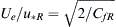. Second, the outer-flow velocity defect law (12.84):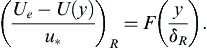

(Ue−U(y)u∗)R=F(yδR).

 

can be vertically integrated from 0 to ∞ to find:

∫0∞(Ue−U(y)u∗)Rdy=∫0∞F(yδR)dy→Ue(u∗)RδR∗=δR∫0∞F(η)dη.

 

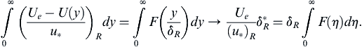
where δR∗ is the displacement thickness of the rough-wall boundary layer. Thus, the argument of the natural logarithm is:

δRu∗Rν=UeδR∗/ν∫0∞F(η)dη≅UeδR∗/ν3.5,

 

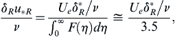
where the integral has been approximately evaluated using the velocity deficit profile shown in Figure 12.20. And third, (12.111) can be used for ΔU⁺ for the purposes of estimation. Substituting these relationships into the mean-velocity-profile-edge equation produces:

2CfR=1κln(UeδR∗/ν3.5)+B+2Πκ−1κln(1+0.26ksUeνCfR2).

 

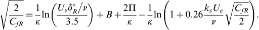
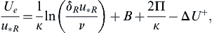
For a ZPG boundary layer, the von Karman boundary-layer integral equation is simply C_f = 2dθ/dx. When integrated and multiplied by the boundary-layer shape factor H, this equation provides an estimate of the boundary-layer displacement thickness in terms of the skin friction:

δR∗(x)=HR∫0x(CfR/2)dx≈HR(CfR/2)x,

 

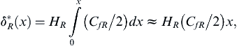
where the approximate equality is valid when H_R and C_fR vary little with increasing x. Although this approximation is not strictly accurate, the inaccuracy it introduces is suppressed by its appearance within the argument of a logarithmic function. Thus, the mean-velocity-profile-edge equation becomes:

2CfR≅1κln((HR/3.5)RexCfR/21+0.26ReksCfR/2)+B+2Πκ,

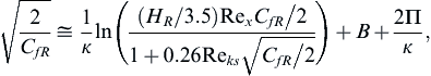(12.114)

 

where Re_x = U_ex/ν and Re_ks = U_ek_s/ν.

This equation can be solved implicitly for C_fR when the other parameters are known. With ν = 10^–6 m²/s, the given information leads to Re_x = 10⁸ and (12.113) leads to k_s = 540 μm, so Re_ks = 5400. Using κ = 0.4, B = 5.0, Π = 0.44, and H_R = 1.3, a generic high-Reynolds number value for the shape factor, (12.114) leads to C_fR ≈ 0.0033.

Interestingly, as shown on Figure 12.25, C_fR from (12.114) calculated with Re_ks = 0 (and the other constants as specified in this example) falls within 2% of the more modern smooth-wall skin friction results from (12.93) evaluated with the log-law constants recommended by Marusic et al. (2013), κ = 0.39 and B = 4.3. Plus, (12.114) provides C_fR values that are within +3 and –6% of the classical rough-wall data correlations found in Schlichting (1979) for the fully rough regime when 10² ≤ x/k_s ≤ 10⁶ (see Exercise 12.41).

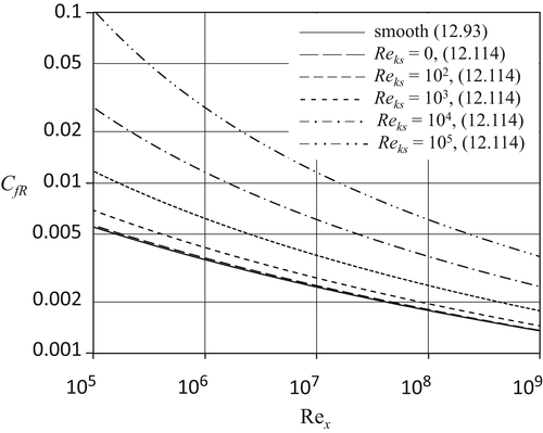
Figure 12.25 Rough surface skin friction coefficient, C_fR, for a zero-pressure-gradient flat-plate turbulent boundary layer vs. Re_x, the Reynolds number based on downstream distance. The solid curve corresponds to (12.93) evaluated using log-law constants κ = 0.39 and B = 4.3 (as recommended by Marusic et al., 2013). The dashed and dash-dot curves come from implicit evaluation of (12.114) for equivalent-sand-grain roughness-height Reynolds numbers of Re_ks = 0, 10², 10³, 10⁴, and 10⁵. The C_fR values produced by (12.114) agree within engineering accuracy (± 5% or so) with prior rough-plate results.