But it should always be required that a mathematical subject not be considered exhausted until it has become intuitively evident…
FELIX KLEIN
Prior to and during the work on non-Euclidean geometry, the study of projective properties was the major geometric activity. Moreover, it was evident from the work of von Staudt (Chap. 35, sec. 3) that projective geometry is logically prior to Euclidean geometry because it deals with qualitative and descriptive properties that enter into the very formation of geometrical figures and does not use the measures of line segments and angles. This fact suggested that Euclidean geometry might be some specialization of projective geometry. With the non-Euclidean geometries now at hand the possibility arose that these, too, at least the ones dealing with spaces of constant curvature, might be specializations of projective geometry. Hence the relationship of projective geometry to the non-Euclidean geometries, which are metric geometries because distance is employed as a fundamental concept, became a subject of research. The clarification of the relationship of projective geometry to Euclidean and the non-Euclidean geometries is the great achievement of the work we are about to examine. Equally vital was the establishment of the consistency of the basic non-Euclidean geometries.
The non-Euclidean geometries that seemed to be most significant after Riemann’s work were those of spaces of constant curvature. Riemann himself had suggested in his 1854 paper that a space of constant positive curvature in two dimensions could be realized on a surface of a sphere provided the geodesic on the sphere was taken to be the “straight line.” This non-Euclidean geometry is now referred to as double elliptic geometry for reasons which will be clearer later. Prior to Riemann’s work, the non-Euclidean geometry of Gauss, Lobatchevsky, and Bolyai, which Klein later called
hyperbolic geometry, had been introduced as the geometry in a plane in which ordinary (and necessarily infinite) straight lines are the geodesies. The relationship of this geometry to Riemann’s varieties was not clear. Riemann and Minding1 had thought about surfaces of constant negative curvature but neither man related these to hyperbolic geometry.
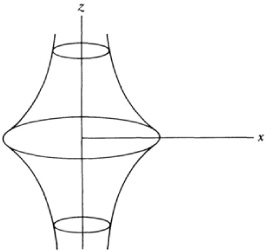
Independently of Riemann, Beltrami recognized2 that surfaces of constant curvature are non-Euclidean spaces. He gave a limited representation of hyperbolic geometry on a surface,3 which showed that the geometry of a restricted portion of the hyperbolic plane holds on a surface of constant negative curvature if the geodesies on this surface are taken to be the straight lines. The lengths and angles on the surface are the lengths and angles of the ordinary Euclidean geometry on the surface. One such surface is known as the pseudosphere (Fig. 38.1). It is generated by revolving a curve called the tractrix about its asymptote. The equation of the tractrix is
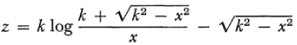
and the equation of the surface is
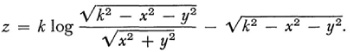
The curvature of the surface is — 1 /?2. Thus the pseudosphere is a model for a limited portion of the plane of Gauss, Lobatchevsky, and Bolyai. On the pseudosphere a figure may be shifted about and just bending will make it conform to the surface, as a plane figure by bending can be fitted to the surface of a circular cylinder.
Beltrami had shown that on a surface of negative constant curvature one can realize a piece of the Lobatchevskian plane. However, there is no regular analytic surface of negative constant curvature on which the geometry of the entire Lobatchevskian plane is valid. All such surfaces have a singular curve— the tangent plane is not continuous across it—so that a continuation of the surface across this curve will not continue the figures that represent those of Lobatchevsky’s geometry. This result is due to Hilbert.4
In this connection it is worth noting that Heinrich Liebmann (1874— 1939)5 proved that the sphere is the only closed analytic surface (free of singularities) of constant positive curvature and so the only one that can be used as a Euclidean model for double elliptic geometry.
The development of these models helped the mathematicians to understand and see meaning in the basic non-Euclidean geometries. One must keep in mind that these geometries, in the two-dimensional case, are fundamentally geometries of the plane in which the lines and angles are the usual lines and angles of Euclidean geometry. While hyperbolic geometry had been developed in this fashion, the conclusions still seemed strange to the mathematicians and had been only grudgingly admitted into mathematics. The double elliptic geometry, suggested by Riemann’s differential geometric approach, did not even have an axiomatic development as a geometry of the plane. Hence the only meaning mathematicians could see for it was that provided by the geometry on the sphere. A far better understanding of the nature of these geometries was secured through another development that sought to relate Euclidean and projective geometry.
Though Poncelet had introduced the distinction between projective and metric properties of figures and had stated in his Traité of 1822 that the projective properties were logically more fundamental, it was von Staudt who began to build up projective geometry on a basis independent of length and angle size (Chap. 35, sec. 3). In 1853 Edmond Laguerre (1834-86), a professor at the Collège de France, though primarily interested in what happens to angles under a projective transformation, actually advanced the goal of establishing metric properties of Euclidean geometry on the basis of projective concepts by supplying a projective basis for the measure of an angle.6
To obtain a measure of the angle between two given intersecting lines one can consider two lines through the origin and parallel respectively to the two given lines. Let the two lines through the origin have the equations (in nonhomogeneous coordinates) y = x tan θ and y = x tan θ’. Let y = ix and y = —ix be two (imaginary) lines from the origin to the circular points at infinity, that is, the points (1, i, 0) and (1, — i, 0). Call these four lines u, u′, w, and w′ respectively. Let Φ be the angle between u and u′. Then Laguerre’s result is that
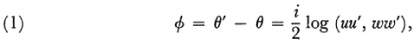
where (uu′, ww′) is the cross ratio of the four lines.7 What is significant about the expression (1) is that it may be taken as the definition of the size of an angle in terms of the projective concept of cross ratio. The logarithm function is, of course, purely quantitative and may be introduced in any geometry.
Independently of Laguerre, Cayley made the next step. He approached geometry from the standpoint of algebra, and in fact was interested in the geometric interpretation of quantics (homogeneous polynomial forms), a subject we shall consider in Chapter 39. Seeking to show that metrical notions can be formulated in projective terms he concentrated on the relation of Euclidean to projective geometry. The work we are about to describe is in his “Sixth Memoir upon Quantics.”8
Cayley’s work proved to be a generalization of Laguerre’s idea. The latter had used the circular points at infinity to define angle in the plane. The circular points are really a degenerate conic. In two dimensions Cayley introduced any conic in place of the circular points and in three dimensions he introduced any quadric surface. These figures he called the absolutes. Cayley asserted that all metric properties of figures are none other than projective properties augmented by the absolute or in relation to the absolute. He then showed how this principle led to a new expression for angle and an expression for distance between two points.
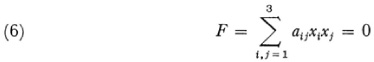
He starts with the fact that the points of a plane are represented by homogeneous coordinates. These coordinates are not to be regarded as distances or ratios of distances but as an assumed fundamental notion not requiring or admitting of explanation. To define distance and size of angle he introduces the quadratic form
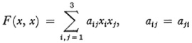
and the bilinear form
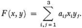
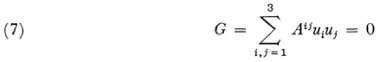
The equation F(x, x) = 0 defines a conic which is Cayley’s absolute. The equation of the absolute in line coordinates is
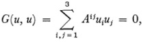
where Aij3 is the cofactor of au in the determinant |a| of the coefficients ofF.
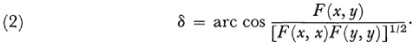
Cayley now defines the distance δ between two points x and y, where x = (x1, x2, x3} and y = (y1, y2, y3), by the formula
The angle Φ between two lines whose line coordinates are ? = (uu1, u2, u3) and v = (v1, v2,3) is defined by
These general formulas become simple if we take for the absolute the particular conic  . Then if (a1, a2, a3) and (b1, b2, b3) are the homogeneous coordinates of two points, the distance between them is given by
and the angle Φ between two lines whose homogeneous line coordinates are (u1, u2, u3) and (v1, v2, v3) is given by
With respect to the expression for distance if we use the shorthand that xy = x1y1 + x2y2 + x3y3 then, if a =(a1, a2, a3), b and c are three points on a line.
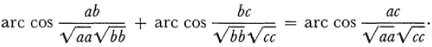
That is, the distances add as they should. By taking the absolute conic to be the circular points at infinity, (1, i, 0) and (1, —i, 0), Cayley showed that his formulas for distance and angle reduce to the usual Euclidean formulas.
It will be noted that the expressions for length and angle involve the algebraic expression for the absolute. Generally the analytic expression of any Euclidean metrical property involves the relation of that property to the absolute. Metrical properties are not properties of the figure per se but of the figure in relation to the absolute. This is Cayley’s idea of the general projective determination of metrics. The place of the metric concept in projective geometry and the greater generality of the latter were described by Cayley as, “Metrical geometry is part of projective geometry.”
Cayley’s idea was taken over by Felix Klein (1849-1925) and generalized so as to include the non-Euclidean geometries. Klein, a professor at Göttingen, was one of the leading mathematicians in Germany during the last part of the nineteenth and first part of the twentieth century. During the years 1869-70 he learned the work of Lobatchevsky, Bolyai, von Staudt, and Cayley; however, even in 1871 he did not know Laguerre’s result. It seemed to him to be possible to subsume the non-Euclidean geometries, hyperbolic and double elliptic geometry, under projective geometry by exploiting Cayley’s idea. He gave a sketch of his thoughts in a paper of 1871 9 and then developed them in two papers.10 Klein was the first to recognize that we do not need surfaces’ to obtain models of non-Euclidean geometries.
To start with, Klein noted that Cayley did not make clear just what he had in mind for the meaning of his coordinates. They were either simply variables with no geometrical interpretation or they were Euclidean distances. But to derive the metric geometries from projective geometry it was necessary to build up the coordinates on a projective basis. Von Staudt had shown (Chap. 35, sec. 3) that it was possible to assign numbers to points by his algebra of throws. But he used the Euclidean parallel axiom. It seemed clear to Klein that this axiom could be dispensed with and in the 1873 paper he shows that this can be done. Hence coordinates and cross ratio of four points, four lines, or four planes can be defined on a purely projective basis.
Klein’s major idea was that by specializing the nature of Cayley’s absolute quadric surface (if one considers three-dimensional geometry) one could show that the metric, which according to Cayley depended on the nature of the absolute, would yield hyperbolic and double elliptic geometry. When the second degree surface is a real ellipsoid, real elliptic paraboloid, or real hyperboloid of two sheets one gets Lobatchevsky’s metric geometry, and when the second degree surface is imaginary one gets Riemann’s non-Euclidean geometry (of constant positive curvature). If the absolute is
taken to be the sphere-circle, whose equation in homogeneous coordinates is x2 + y2 + z2 = 0, t = 0, then the usual Euclidean metric geometry obtains. Thus the metric geometries become special cases of projective geometry.
To appreciate Klein’s ideas let us consider two-dimensional geometry. One chooses a conic in the projective plane; this conic will be the absolute. Its equation is
in point coordinates and
in line coordinates. To derive Lobatchevsky’s geometry the conic must be real, e.g. in plane homogeneous coordinates  for Riemann’s geometry on a surface of constant positive curvature it is imaginary, for example, and for Euclidean geometry, the conic degenerates into two coincident lines represented in homogeneous coordinates by x3 = 0, and on this locus one chooses two imaginary points whose equation is
  that is, the circular points at infinity whose homogeneous coordinates are (I, i, 0) and (1, — ¿, 0). In every case the conic has a real equation.
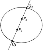
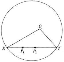
To be specific let us suppose the conic is the one shown in Figure 38.2. If P1 and P2 are two points of a line, this line meets the absolute in two points (real or imaginary). Then the distance is taken to be

where the quantity in parentheses denotes the cross ratio of the four points and c is a constant. This cross ratio can be expressed in terms of the
ordinates of the points. Moreover, if there are three points P1, P2, P3 on the line then it can readily be shown that
(P1P2 Q1Q2) · (P2P3 Q1Q2) = (P1P3 Q1Q2)
so that P1P2 + P2P3 = P1P3
so that P1P2 + P2P3 = P1P3
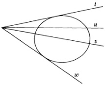
Likewise if u and v are two lines (Fig. 38.3) one considers the tangents t and w from their point of intersection to the absolute (the tangents may be imaginary lines); then the angle between ? and ? is defined to be
Φ = c′ log (uv, tw),
where again c′ is a constant and the quantity in parentheses denotes the cross ratio of the four lines.
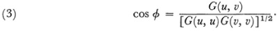
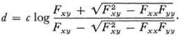
To express the values of d and Φ analytically and to show their dependence upon the choice of the absolute, let the equation of the absolute be given by F and G above. By definition
One can now show that if x = (x1, x2, x3) and y = (y1, y2, y3) are the coordinates of P1 and P2 then
Likewise, if (u1, u2, u3) and (v1, v2, v3) are the coordinates of the two lines, then one can show, using G, that
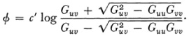
The constant c′ is generally taken to be i/2 so as to make φ real and a complete central angle 2π
Klein used the logarithmic expressions above for angle and distance and showed how the metric geometries can be derived from projective geometry.
Thus if one starts with projective geometry then by his choice of the absolute and by using the above expressions for distance and angle one can get the Euclidean, hyperbolic, and elliptic geometries as special cases. The nature of the metric geometry is fixed by the choice of the absolute. Incidentally, Klein’s expressions for distance and angle can be shown to be equal to Cayley’s.
If one makes a projective (i.e. linear) transformation of the projective plane into itself which transforms the absolute into itself (though points on the absolute go into other points) then because cross ratio is unaltered by a linear transformation, distance and angle will be unaltered. These particular linear transformations which leave the absolute fixed are the rigid motions or congruence transformations of the particular metric geometry determined by the absolute. A general projective transformation will not leave the absolute invariant. Thus projective geometry proper is more general in the transformations it allows.
Another contribution of Klein to non-Euclidean geometry was the observation, which he says he first made in 187111 but published in 1874,12that there are two kinds of elliptic geometry. In the double elliptic geometry two points do not always determine a unique straight line. This is evident from the spherical model when the two points are diametrically opposite. In the second elliptic geometry, called single elliptic, two points always determine a unique straight line. When looked at from the standpoint of differential geometry, the differential form ds2 of a surface of constant positive curvature is (in homogeneous coordinates)
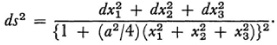
In both cases a2 > 0. However, in the first type the geodesies are curves of finite length 2π/a or if R is the radius, 2πR, and are closed (return upon themselves). In the second the geodesies are of length π/a or πR and are still closed.
A model of a surface which has the properties of single elliptic geometry and which is due to Klein,13 is provided by a hemisphere including the boundary. However, one must identify any two points on the boundary which are diametrically opposite. The great circular arcs on the hemisphere are the “straight lines” or geodesies of this geometry and the ordinary angles on the surface are the angles of the geometry. Single elliptic geometry (sometimes called elliptic in which case double elliptic geometry is called spherical) is then also realized on a space of constant positive curvature.
One cannot actually unite the pairs of points which are identified in this model at least in three-dimensional space. The surface would have to cross itself and points that coincide on the intersection would have to be regarded as distinct.
We can now see why Klein introduced the terminology hyperbolic for Lobatchevsky’s geometry, elliptic for the case of Riemann’s geometry on a surface of constant positive curvature, and parabolic for Euclidean geometry. This terminology was suggested by the fact that the ordinary hyperbola meets the line at infinity in two points and correspondingly in hyperbolic geometry each line meets the absolute in two real points. The ordinary ellipse has no real points in common with the line at infinity and in elliptic geometry, likewise, each line has no real points in common with the absolute. The ordinary parabola has only one real point in common with the line at infinity and in Euclidean geometry (as extended in projective geometry) each line has one real point in common with the absolute.
The import which gradually emerged from Klein’s contributions was that projective geometry is really logically independent of Euclidean geometry. Moreover, the non-Euclidean and Euclidean geometries were also seen to be special cases or subgeometries of projective geometry. Actually the strictly logical or rigorous work on the axiomatic foundations of projective geometry and its relations to the subgeometries remained to be done (Chap. 42). But by making apparent the basic role of projective geometry Klein paved the way for an axiomatic development which could start with projective geometry and derive the several metric geometries from it.
By the early 1870s several basic non-Euclidean geometries, the hyperbolic and the two elliptic geometries, had been introduced and intensively studied. The fundamental question which had yet to be answered in order to make these geometries legitimate branches of mathematics was whether they were consistent. All of the work done by Gauss, Lobatchevsky, Bolyai, Riemann, Cayley, and Klein might still have proved to be nonsense if contradictions were inherent in these geometries.
Actually the proof of the consistency of two-dimensional double elliptic geometry was at hand, and possibly Riemann appreciated this fact though he made no explicit statement. Beltrami14 had pointed out that Riemann’s two-dimensional geometry of constant positive curvature is realized on a sphere. This model makes possible the proof of the consistency of two-dimensional double elliptic geometry. The axioms (which were not explicit at this time) and the theorems of this geometry are all applicable to the geometry of the surface of the sphere provided that line in the double elliptic geometry is interpreted as great circle on the surface of the sphere. If there should be contradictory theorems in this double elliptic geometry then there would be contradictory theorems about the geometry of the surface of the sphere. Now the sphere is part of Euclidean geometry. Hence if Euclidean geometry is consistent, then double elliptic geometry must also be so. To the mathematicians of the 1870s the consistency of Euclidean geometry was hardly open to question because, apart from the views of a few men such as Gauss, Bolyai, Lobatchevsky, and Riemann, Euclidean geometry was still the necessary geometry of the physical world and it was inconceivable that there could be contradictory properties in the geometry of the physical world. However, it is important, especially in the light of later developments, to realize that this proof of the consistency of double elliptic geometry depends upon the consistency of Euclidean geometry.
The method of proving the consistency of double elliptic geometry could not be used for single elliptic geometry or for hyperbolic geometry. The hemispherical model of single elliptic geometry cannot be realized in three-dimensional Euclidean geometry though it can be in four-dimensional Euclidean geometry. If one were willing to believe in the consistency of the latter, then one might accept the consistency of single elliptic geometry. However, though ?-dimensional geometry had already been considered by Grassmann, Riemann, and others, it is doubtful that any mathematician of the 1870s would have been willing to affirm the consistency of four-dimensional Euclidean geometry.
The case for the consistency of hyperbolic geometry could not be made on any such grounds. Beltrami had given the pseudospherical interpretation, which is a surface in Euclidean space, but this serves as a model for only a limited region of hyperbolic geometry and so could not be used to establish the consistency of the entire geometry. Lobatchevsky and Bolyai had considered this problem (Chap. 36, sec. 8) but had not been able to settle it. As a matter of fact, though Bolyai proudly published his non-Euclidean geometry, there is evidence that he doubted its consistency because in papers found after his death he continued to try to prove the Euclidean parallel axiom.
The consistency of the hyperbolic and single elliptic geometries was established by new models. The model for hyperbolic geometry is due to Beltrami.15 However, the distance function used in this model is due to Klein and the model is often ascribed to him. Let us consider the two-dimensional case.
Within the Euclidean plane (which is part of the projective plane) one selects a real conic which one may as well take to be a circle (Fig. 38.4).
According to this representation of hyperbolic geometry the points of the geometry are the points interior to this circle. A line of this geometry is a chord of the circle, say the chord XY (but not including X and F). If we take any point Q not on XY then we can find any number of lines through Q which do not meet XY. Two of these lines, namely, QX and QY, separate the lines through Q into two classes, those lines which cut XY and those which do not. In other words, the parallel axiom of hyperbolic geometry is satisfied by the points and lines (chords) interior to the circle. Further, let the size of the angle formed by two lines a and b be
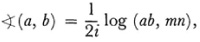
where m and n are the conjugate imaginary tangents from the vertex of the angle to the circle and (ab, mn) is the cross ratio of the four lines a, b, m, and n. The constant 1/2i’ ensures that a right angle has the measure π/2. The definition of distance between two points is given by formula (8), that is, d = c log (P1P2, XT) with c usually taken to be k/2. According to this formula as P1 or P2 approaches X or T, the distance P¡P2 becomes infinite. Hence in terms of this distance, a chord is an infinite line of hyperbolic geometry.
Thus with the projective definitions of distance and angle size, the points, chords, angles, and other figures interior to the circle satisfy the axioms of hyperbolic geometry. Then the theorems of hyperbolic geometry also apply to these figures inside the circle. In this model the axioms and theorems of hyperbolic geometry are really assertions about special figures and concepts (e.g. distance defined in the manner of hyperbolic geometry) of Euclidean geometry. Since the axioms and theorems in question apply to these figures and concepts, regarded as belonging to Euclidean geometry, all of the assertions of hyperbolic geometry are theorems of Euclidean geometry. If, then, there were a contradiction in hyperbolic geometry, this contradiction would be a contradiction within Euclidean geometry. But if Euclidean geometry is consistent, then hyperbolic geometry must also be. Thus the
consistency of hyperbolic geometry is reduced to the consistency of Euclidean geometry.
The fact that hyperbolic geometry is consistent implies that the Euclidean parallel axiom is independent of the other Euclidean axioms. If this were not the case, that is, if the Euclidean parallel axiom were derivable from the other axioms, it would also be a theorem of hyperbolic geometry for, aside from the parallel axiom, the other axioms of Euclidean geometry are the same as those of hyperbolic geometry. But this theorem would contradict the parallel axiom of hyperbolic geometry and hyperbolic geometry would be inconsistent. The consistency of two-dimensional single elliptic geometry can be shown in the same manner as for hyperbolic geometry because this elliptic geometry is also realized within the projective plane and with the projective definition of distance.
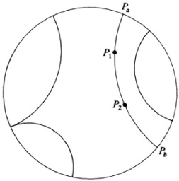
Independently and in connection with his work on automorphic functions Poincaré16 gave another model which also establishes the consistency of hyperbolic geometry. One form in which this Poincaré model for hyperbolic plane geometry17 can be expressed takes the absolute to be a circle (Fig. 38.5). Within the absolute the straight lines of the geometry are arcs of circles which cut the absolute orthogonally and straight lines through the center of the absolute. The length of any segment P1P2 is given by log (P1P2, PaPb), where (P1P2, PaPb) = (P1P2,/PaPb) Pa and Pb are the chords. The angle between two intersecting “lines” of this model is the normal Euclidean angle between the two arcs. Two circular arcs which are tangent at a point on the absolute are parallel
“lines.” Since in this model, too, the axioms and theorems of hyperbolic geometry are special theorems of Euclidean geometry, the argument given above apropos of the Beltrami model may be applied here to establish the consistency of hyperbolic geometry. The higher-dimensional analogues of the above models are also valid.
Klein’s success in subsuming the various metric geometries under projective geometry led him to seek to characterize the various geometries not just on the basis of nonmetric and metric properties and the distinctions among the metrics but from the broader standpoint of what these geometries and other geometries which had already appeared on the scene sought to accomplish. He gave this characterization in a speech of 1872, “Vergleichende Betrachtungen über neuere geometrische Forschungen” (A Comparative Review of Recent Researches in Geometry),18 on the occasion of his admission to the faculty of the University of Erlangen, and the views expressed in it are known as the Erlanger Programm.
Klein’s basic idea is that each geometry can be characterized by a group of transformations and that a geometry is really concerned with invariants under this group of transformations. Moreover a subgeometry of a geometry is the collection of invariants under a subgroup of transformations of the original group. Under this definition all theorems of a geometry corresponding to a given group continue to be theorems in the geometry of the subgroup.
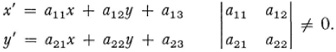
Though Klein in his paper does not give the analytical formulations of the groups of transformations he discusses we shall give some for the sake of explicitness. According to his notion of a geometry projective geometry, say in two dimensions, is the study of invariants under the group of transformations from the points of one plane to those of another or to points of the same plane (collineations). Each transformation is of the form
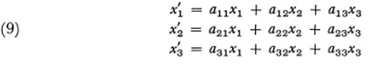
wherein homogeneous coordinates are presupposed, the au are real numbers, and the determinant of the coefficients must not be zero. In nonhomo-geneous coordinates the transformations are represented by
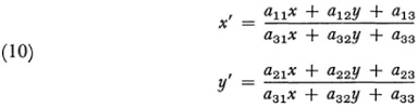
and again the determinant of the a{¡ must not be zero. The invariants under the projective group are, for example, linearity, collinearity, cross ratio, harmonic sets, and the property of being a conic section.
One subgroup of the projective group is the collection of affine transformations.19 This subgroup is defined as follows: Let any line lm in the projective plane be fixed. The points of l∞ are called ideal points or points at infinity and lw is called the line at infinity. Other points and lines of the projective plane are called ordinary points and these are the usual points of the Euclidean plane. The affine group of collineations is that subgroup of the projective group which leaves invariant (though not necessarily pointwise) and affine geometry is the set of properties and relations invariant under the affine group. Algebraically, in two dimensions and in homogeneous coordinates, the affine transformations are represented by equations (9) above but in which a31 = a 32 = 0 and with the same determinant condition. In nonhomogeneous coordinates affine transformations are given by
Under an affine transformation, straight lines go into straight lines, and parallel straight lines into parallel lines. However, lengths and angle sizes are altered. Affine geometry was first noted by Euler and then by Möbius in his Der bary centrische Calcul. It is useful in the study of the mechanics of deformations.
The group of any metric geometry is the same as the affine group except that the determinant above must have the value +1 or — 1. The first of the metric geometries is Euclidean geometry. To define the group of this geometry one starts with lx and supposes there is a fixed involution on l∞. One requires that this involution has no real double points but has the circular points at oo as (imaginary) double points. We now consider all projective transformations which not only leave l∞ fixed but carry any point of the involution into its corresponding point of the involution, which implies that each circular point goes into itself. Algebraically these transformations of the Euclidean group are represented in nonhomogeneous (two-dimensional) coordinates by
The invariants are length, size of angle, and size and shape of any figure.
Euclidean geometry as the term is used in this classification is the set of invariants under this class of transformations. The transformations are rotations, translations, and reflections. To obtain the invariants associated with similar figures, the subgroup of the affine group known as the parabolic
metric group is introduced. This group is defined as the class of projective transformations which leaves the involution on la invariant, and this means that each pair of corresponding points goes into some pair of corresponding points. In nonhomogeneous coordinates the transformations of the parabolic metric group are of the form
x’ = ax — by + c
y’ = bex + aey + d
wherein a2 + b2 ≡ 0, and e2 = 1. These transformations preserve angle size.
To characterize hyperbolic metric geometry we return to projective geometry and consider an arbitrary, real, nondegenerate conic (the absolute) in the projective plane. The subgroup of the projective group which leaves this conic invariant (though not necessarily pointwise) is called the hyperbolic metric group and the corresponding geometry is hyperbolic metric geometry. The invariants are those associated with congruence.
Single elliptic geometry is the geometry corresponding to the subgroup of projective transformations which leaves a definite imaginary ellipse (the absolute) of the projective plane invariant. The plane of elliptic geometry is the real projective plane and the invariants are those associated with congruence.
Even double elliptic geometry can be encompassed in this transformation viewpoint, but one must start with three-dimensional projective transformations to characterize the two-dimensional metric geometry. The subgroup of transformations consists of those three-dimensional projective transformations which transform a definite sphere (surface) S of the finite portion of space into itself. The spherical surface S is the “plane” of double elliptic geometry. Again the invariants are associated with congruence.
In four metric geometries, that is, Euclidean, hyperbolic, and the two elliptic geometries, the transformations which are permitted in the corresponding subgroup are what are usually called rigid motions and these are the only geometries which permit rigid motions.
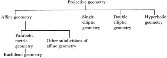
Klein introduced a number of intermediate classifications which we shall not repeat here. The scheme below shows the relationships of the principal geometries.
Klein also considered more general geometries than projective. At this time (1872) algebraic geometry was gradually being distinguished as a separate discipline and he characterized this geometry by introducing the transformations which in three dimensions and in nonhomogeneous coordinates read
x’ = Φ(x, y, z), y’ = ψ(x, y, z), z’ = X(x, y, z).
He required that the functions Φ, ψ, and x be rational and single-valued and that it must be possible to solve for x, y, and z in terms of single-valued rational functions of x′, y′, z′. These transformations are called Cremona transformations and the invariants under them are the subject matter of algebraic geometry (Chap. 39).
Klein also projected the study of invariants under one-to-one continuous transformations with continuous inverses. This is the class now called homeomorphisms and the study of the invariants under such transformations is the subject matter of topology (Chap. 50). Though Riemann had also considered what are now recognized to be topological problems in his work with Riemann surfaces, the projection of topology as a major geometry was a bold step in 1872.
It has been possible since Klein’s days to make further additions and specializations of Klein’s classification. But not all of geometry can be incorporated in Klein’s scheme. Algebraic geometry today and differential geometry do not come under this scheme.20 Though Klein’s view of geometry did not prove to be all-embracing, it did afford a systematic method of classifying and studying a good portion of geometry and suggested numerous research problems. His “definition” of geometry guided geometrical thinking for about fifty years. Moreover, his emphasis on invariants under transformations carried beyond mathematics to mechanics and mathematical physics generally. The physical problem of invariance under transformation or the problem of expressing physical laws in a manner independent of the coordinate system became important in physical thinking after the invariance of Maxwell’s equations under Lorentz transformations (a four-dimensional subgroup of affine geometry) was noted. This line of thinking led to the special theory of relativity.
We shall merely mention here further studies on the classification of geometries which at least in their time attracted considerable attention. Helmholtz and Sophus Lie (1842-99) sought to characterize geometries in which rigid motions are possible. Helmholtz’s basic paper, “Uber die Thatsachen, die der Geometrie zum Grunde liegen” (On the Facts Which Underlie Geometry),21 showed that if the motions of rigid bodies are to be possible in a space then Riemann’s expression for ds in a space of constant curvature is the only one possible. Lie attacked the same problem by what is called the theory of continuous transformation groups, a theory he had already introduced in the study of ordinary differential equations, and he characterized the spaces in which rigid motions are possible by means of the kinds of groups of transformations which these spaces permit.22
The interest in the classical synthetic non-Euclidean geometries and in projective geometry declined after the work of Klein and Lie partly because the essence of these structures was so clearly exposed by the transformation viewpoint. The feeling of mathematicians so far as the discovery of additional theorems is concerned was that the mine had been exhausted. The rigoriza-tion of the foundations remained to be accomplished and this was an active area for quite a few years after 1880 (Chap. 42).
Another reason for the loss of interest in the non-Euclidean geometries was their seeming lack of relevance to the physical world. It is curious that the first workers in the field, Gauss, Lobatchevsky, and Bolyai did think that non-Euclidean geometry might prove applicable when further work in astronomy had been done. But none of the mathematicians who worked in the later period believed that these basic non-Euclidean geometries would be physically significant. Cayley, Klein, and Poincaré, though they considered this matter, affirmed that we would not ever need to improve on or abandon Euclidean geometry. Beltrami’s pseudosphere model had made non-Euclidean geometry real in a mathematical sense (though not physically) because it gave a readily visualizable interpretation of Lobatchevsky’s geometry but at the expense of changing the line from the ruler’s edge to geodesies on the pseudosphere. Similarly the Beltrami-Klein and Poincaré models made sense of non-Euclidean geometry by changing the concepts either of line, distance, or angle-measure, or of all three, and by picturing them in Euclidean space. But the thought that physical space under the usual interpretation of straight line or even under some other interpretation could be non-Euclidean was dismissed. In fact, most mathematicians regarded non-Euclidean geometry as a logical curiosity.
Cayley was a staunch supporter of Euclidean space and accepted the non-Euclidean geometries only so far as they could be realized in Euclidean space by the use of new distance formulas. In 1883 in his presidential address to the British Association for the Advancement of Science23 he said that non-Euclidean spaces were a priori a mistaken idea, but non-Euclidean geometries were acceptable because they resulted merely from a change in the distance function in Euclidean space. He did not grant independent existence to the non-Euclidean geometries but regarded them as a class of special Euclidean structures or as a way of representing projective relations in Euclidean geometry. It was his view that
Euclid’s twelfth [tenth] axiom in Playfair’s form of it does not need demonstration but is part of our notion of space, of the physical space of our own experience—the space, that is, which we become acquainted with by experience, but which is the representation lying at the foundation of all external experience.
Riemann’s view may be said to be that, having in intellectu a more general notion of space (in fact a notion of non-Euclidean space), we learn by experience that space (the physical space of experience) is, if not exactly, at least to the highest degree of approximation, Euclidean space.
Klein regarded Euclidean space as the necessary fundamental space. The other geometries were merely Euclidean with new distance functions. The non-Euclidean geometries were in effect subordinated to Euclidean geometry.
Poincaré’s judgment was more liberal. Science should always try to use Euclidean geometry and vary the laws of physics where necessary. Euclidean geometry may not be true but it is most convenient. One geometry cannot be more true than another; it can only be more convenient. Man creates geometry and then adapts the physical laws to it to make the geometry and laws fit the world. Poincaré insisted24 that even if the angle sum of a triangle should prove to be greater than 180° it would be better to assume that Euclidean geometry describes physical space and that light travels along curves because Euclidean geometry is simpler. Of course events proved he was wrong. It is not the simplicity of the geometry alone that counts for science but the simplicity of the entire scientific theory. Clearly the mathematicians of the nineteenth century were still tied to tradition in their notions about what makes physical sense. The advent of the theory of relativity forced a drastic change in the attitude toward non-Euclidean geometry.
The delusion of mathematicians that what they are working on at the moment is the most important conceivable subject is illustrated again by their attitude toward projective geometry. The work we have examined in this chapter does indeed show that projective geometry is fundamental to many geometries. However, it does not embrace the evidently vital Rie-mannian geometry and the growing body of algebraic geometry. Neverthe less, Cayley affirmed in his 1859 paper (sec. 3) that, “Projective geometry is all geometry and reciprocally.”25 Bertrand Russell in his Essay on the Foundations of Geometry (1897) also believed that projective geometry was necessarily the a priori form of any geometry of physical space. Hermann Hankel, despite the attention he gave to history,26 did not hesitate to say in 1869 that projective geometry is the royal road to all mathematics. Our examination of the developments already recorded shows clearly that mathematicians can readily be carried away by their enthusiasms.
Beltrami, Eugenio: Opere matematiche, Ulrico Hoepli, 1902, Vol. 1.
Bonola, Roberto: Non-Euclidean Geometry, Dover (reprint), 1955, pp. 129-264.
Coolidge, Julian L.: A History of Geometrical Methods, Dover (reprint), 1963, pp. 68-87.
Klein, Felix: Gesammelte mathematische Abhandlungen, Julius Springer, 1921-23, Vols. 1 and 2.
Pasch, Moritz, and Max Dehn: Vorlesungen über neuere Geometrie, 2nd ed., Julius Springer, 1926, pp. 185-239.
Pierpont, James: “Non-Euclidean Geometry. A Retrospect,” Amer. Math. Soc. Bull, 36, 1930, 66-76.
Russell, Bertrand: An Essay on the Foundations of Geometry (1897), Dover (reprint), 1956.