APPENDICES
These appendices present three conceptual models that illustrate some of the ideas in the book. The first is based on bread-making, the second on the flow of air, the third on the growth of daisies. Each tells a simple story, like a fable, and has its own moral.
APPENDIX I: THE SHIFT MAP
The shift map was introduced in Chapter 3 as a simple example of a chaotic system. The dynamics, which are similar to the kneading of bread dough, were illustrated in figure 3.2 (see page 100). The first few iterations, for two nearby initial conditions, are shown in the left panel of figure A.1. The solid and dashed lines could represent the positions of two yeast cells in the dough, on a scale from 0 to 1. They start close together, but after just a few iterations, they are completely separated.
Now, suppose that we wish to predict the future location of the daughter cell (dashed line in the left panel), based on the position of the mother cell (solid line). Over the first few steps, the error will increase exponentially. The solid line in the right panel shows the average error growth over a large number of experiments from different starting points, for the same small initial error of 0.005. The average separation indicates what we could expect the prediction error to be after a certain number of iterations. As seen, the exponential growth eventually saturates at the average distance between two randomly chosen points. This is ID="275">  , or about 0.33. 1
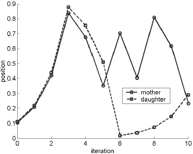
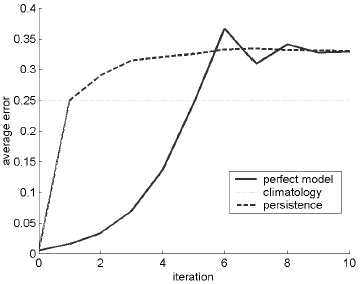
FIGURE A.1. The left panel tracks the location of two yeast cells in dough (on a scale of 0 to 1), separated by 0.005. The distance grows by a factor of two for the first few iterations, then becomes more random. The right panel shows the average or expected error, over a large number of experiments from different starting points, created by a small perturbation to the initial condition. It grows exponentially at first, then saturates at a level equal to the average distance between randomly selected points. The best results for long-term prediction are given by the climatology model, which uses the centre of the dough as its forecast and has an expected error of only 0.25. The dashed line shows error for a persistence forecast, which assumes that the cell stays where it started.
After only a few steps, any prediction performed by applying the shift map is no better than random. A better guess is to use as our “model” the long-term average of all possible states, which is 0.5. This so-called climatological forecast has an average error, for all points including the first, of 0.25, as shown by the dotted line. The dashed line shows error for a persistence forecast, which assumes that the cell stays where it started. For the shift map, we could say that the perfect model (i.e., using the shift map) is best over the short term, while the climatological model is best over the long term. The persistence forecast has no advantages.
The shift map can be represented mathematically as a sequence of transformations. Given an initial condition x0, the next iteration is x1 = mod(2x0), where the mod function means that if 2x0 is greater than 1, only the fractional part is used. This process is repeated, so the nth term in the sequence is given by xn = mod(2xn–1). The shift map is so named because its effect is to shift the binary expansion of the starting point one place to the right. Any point can be represented in a binary expansion as a string of zeros and ones. For example, ½ is 0.1 in binary notation; ID="278">  is 0.01; and ID="279">
  (i.e., ½ + ID="281">
  ) is 0.11.2 Since computers work in zeros and ones, all numbers are converted to binary notation internally. If the initial point in binary notation is x0 = .11010110 . . . , where the higher digits are omitted, then after one step the point will have moved to x1 = .1010110 . . . , x2 = .010110 . . . , and so on.
Another way to view the shift map is therefore as a simple one-dimensional cellular automaton.3 The binary representation of any initial condition can be represented as a line of cells, with white cells corresponding to a 0 and black cells corresponding to a 1. The top line of figure A.2 reads .11010110 . . . , and the lines below show that each iteration just shifts the cells to one side.

FIGURE A.2. Black cells represent 1, white cells represent 0 in a binary expansion. The top line shows the initial condition .11010110 . . . , which is shifted one cell to the left at each iteration of the map.
Our impression of this system depends very much on point of view. If we concentrate on the magnitude of the difference between two points, then we see sensitivity to initial condition and chaotic behaviour. However, if we view the map as operating on a binary expansion, it is just a line of squares marching along, with one falling off the end at each iteration. The system itself is therefore completely predictable. Anyone can compute the effect of a thousand iterations just by shifting the binary representation a thousand places. The only unpredictability—the lack of order and form that the word “chaos” evokes—is a result of error in the measurement of initial condition.
MORAL: Chaotic systems are not the same as complex systems. In the former, prediction requires an accurate initial condition; in the latter, prediction is impossible.
APPENDIX II: THE LORENZ SYSTEM
As discussed in Chapter 4, this system was used by Ed Lorenz from MIT in 1963 to illustrate the effect of chaos on predictability.4 The system is an approximate model of the convective motion of a fluid heated from below and cooled from above, a problem first studied by the Victorian physicist Lord Rayleigh. The differential equations, which express the rate of change of the three variables, are:
dx/dt = – ID="285"> x + y
dy/dt = – xz + Rx – y
dz/dt = xy – Bz
The parameters are usually set to = 10, B = 8/3, and R = 28. The equations were based on a seven-equation model by Barry Saltzman, which itself was truncated from an infinite series of terms derived from a two-dimensional approximation. The system therefore represents an extreme simplification of the actual dynamics.
As shown by the dashed line in figure A.3, the system is sensitive to initial condition: root mean square errors caused by a small change in the initial condition increase in a quasi-exponential fashion with time (as in figure A.1). More significant, though, is the error caused by a 4 percent change in the single parameter R. The relative importance of initial condition and parameter errors depends on the details (and can be measured using the drift technique discussed in Chapter 4), but the point is that the system is sensitive to both. Error cannot necessarily be pinned on the initial values of variables, rather than the parameters. The error in R corresponds to a similar error in the assumed temperature differential of the two plates. In models of the real weather, model error arises not just because of a single parameter, but because the equations themselves cannot reproduce the detailed behaviour of the atmospheric system.
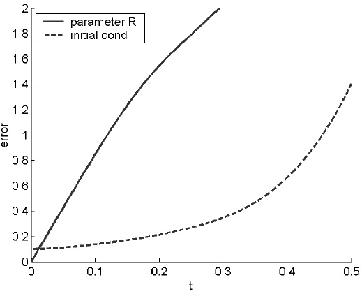
FIGURE A.3. Plot showing root mean square errors caused by a small change of magnitude 0.1 in the initial condition (dashed line) and a 4 percent change in the parameter R from 28 to 29.12 (solid line). Shortterm predictions are sensitive to both initial conditions and parameters. As in the right panel of figure A.1, errors eventually saturate.
Suppose now that the goal is to predict the long-term “climate” of the Lorenz system, in terms of the variance of the fluctuations in x, y, and z. Over the long term, the initial condition is no longer important, because the system settles onto its own attractor; however, the climate depends critically on the parameters and the model equations. A 4 percent increase in R makes the butterfly attractor grow in size, so the variance in each of the three variables increases by about 5 percent—a significant change, since it increases the probability of extreme events.5 The attractor of Saltzman’s original seven-equation model has a completely different appearance—the butterfly grows a body and looks more like a moth.6
The Lorenz system is therefore an example of a chaotic system that is sensitive to changes in parameters and equations when either short- or long-term prediction is the goal. As discussed in Chapter 7, models of the real climate show similar properties.
MORAL:In the long run, and often the short run too, errors in equations matter more than initial errors in the variables—even in chaotic systems.7
APPENDIX III: DAISYWORLD
Daisyworld is a mathematical model that illustrates self-regulating, homeostatic behaviour and represents a simple example of an ecosystem. It was initially developed by James Lovelock and Andrew Watson as a defence of Gaia theory.8 This theory was based on the observation that the earth system seemed to regulate itself like a biological organism. Perhaps taking the idea a little too literally, some mistakenly interpreted it as a claim that the earth was behaving with a sense of purpose, that it was a teleological being actively controlling the climate and so on.9 The purpose of Daisyworld was to show that homeostatic behaviour could emerge naturally, without recourse to teleology. It also exhibits a number of other properties that are typical of models of living systems.
On Daisyworld, an imaginary planet, there are only two species of life: light daisies and dark daisies. Light daisies tend to reflect light, which has a cooling effect, while dark ones absorb radiation, and therefore warm the planet. Growth of the daisies depends on the present population, the natural death rate, the available space, and the temperature. The equations are based on the dynamics of real daisy growth. Details about the equations, as well as animated simulations, can be found at a number of websites.10
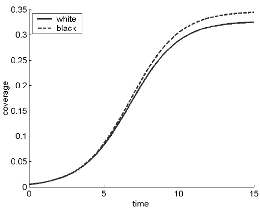
FIGURE A.4. Plot showing the growth of white and black daisies, from an initial seeding. The proportion of white and black daisies at equilibrium acts to regulate the planetary temperature.
Figure A.4 shows a simulation of the growth of the two species, from the initial seeding to their equilibrium level. (The model was also used to obtain the S-shaped curve for economic growth in figure 6.1 on page 237.) The growth can be described in three parts. At first, the seeded daisies grow exponentially, multiplying rapidly and establishing themselves on the planet. In the second phase, growth is complicated by lack of space and competition with other daisies—negative feedback. Finally, in the third phase, the daisies obtain a balanced equilibrium. Life processes still go on, but the number of births is balanced by the number of deaths, so there is no net growth. More complicated versions produce chaotic fluctuations around a mean.
The aim of the model was to illustrate the idea of planetary homeostasis—in particular, how the earth could regulate its temperature as the sun’s luminosity slowly increased. The Daisyworld planet revolves around a sun, absorbing energy at a rate that depends on the sun’s luminosity and the albedo of the planet. It also radiates heat out to the universe, just as the earth does. Black daisies absorb heat and do best in cool conditions. When the planet is cool, they grow more quickly. But in doing so, they lower the albedo of the planet as a whole, thus warming the planet. Similarly, if the planet gets too hot, it will be cooled by the growth of white daisies, which (like polar ice) reflect heat. The two species therefore act antagonistically. Since they are also in competition for space, growth in one tends to repress growth in the other. The final temperature represents a compromise between the two types of daisies—neither too hot, nor too cold. When the model is run with the sun’s luminosity gradually increasing, the light and dark daisies adjust themselves naturally to keep the temperature constant at the optimal level for daisy growth.
Daisyworld is therefore an example of a self-regulating system, where internal conflict between opposing forces somehow conspires to maintain the conditions suitable for life. From the outside, it seems that little is happening; the daisies of different species carry on their lives in balance with each other. Yet stability can be deceptive. Powerful forces are at work to maintain that tranquility in the face of external changes. As Heraclitus wrote: “An invisible harmony is stronger than a visible one.”11 One consequence is that the Daisyworld “climate” is insensitive to changes in initial conditions but sensitive to changes in parameters. This is illustrated in figure A.5, which shows the reaction to different kinds of perturbations. The vertical axis represents the temperature of the white daisies, which has a steady state indicated by the square symbols (as mentioned above, more complex versions produce fluctuations around a mean; homeostasis implies regulation but not static behaviour). If the initial daisy population is increased by 10 percent, competition for space means that the excess daisies die off and equilibrium is rapidly restored (circle symbols). The rate of return depends on the rates of growth and decay, and the steady state represents a balance between these opposing forces. A smaller 2 percent change in a single parameter, which controls the death rate of the white daisies, is enough to create a significant shift in the balance between the two species and affect the temperature (diamond symbols). Note that this does not represent some defect in the equations, but instead is a natural property of the system itself. As an archer takes aim, his two arms similarly pull in opposite directions to tension the bow, and balance each other without conscious direction on his part. The bow is at rest, and from the outside it again looks as if little is happening. But any mathematical model of his movements would be unstable to small random errors in the simulation of the force applied by either hand.
The yeast galactose model discussed in Chapter 5 has some similar dynamics, with the two species of regulatory proteins playing the role of daisies. The rapid growth/decay rates of these species, combined with their opposing regulatory effects, results in a homeostatic system that is highly resistant to both external perturbations and internal stochastic noise (but sensitive to changes in parameters). Since most of the parameters could only be estimated to within about a factor of ten, they had to be carefully balanced against one another to make the model work.
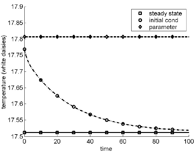
FIGURE A.5. Plot showing sensitivity to parameterization but insensitivity to initial condition, in the Daisyworld system. The normal system has a steady state attractor (square symbols), and a perturbation of 10 percent in the initial condition is rapidly damped out (circle symbols). However, a 2 percent error in one of the parameters results in a new and significantly different steady state (diamond symbols). The reason is that the steady state represents an equilibrium between opposing forces, and it’s easily disturbed by a small error modelling one of them. Note that in most biological systems, it is impossible to measure parameters to anything like 2 percent accuracy.
Daisyworld is only a kind of thought experiment, but it shows how self-regulation can occur without any recourse to teleology. Species in an ecosystem can be concerned with nothing more than their own survival, yet they help not only themselves but the whole system. Daisyworld opened people’s eyes to similar regulatory loops in our own planet. An example is the salinity of the oceans, which is about 3.4 percent.12 Tears from your eyes are about as salty, and most living organisms maintain a salinity that is roughly equal to that of the oceans. Perhaps this is why Empedocles proposed the metaphor that the sea is the sweat of the earth, which so annoyed Aristotle.
One theory about salinity was that natural selection tended to assist those organisms that were in balance with their surroundings. So why has the ocean managed to maintain a constant level of salinity? If it were to go much above 4 percent, then basic cell functions, such as the electromagnetic potential maintained across cell membranes, would fail. There would be mass extinctions of life in the oceans. And yet there is no evidence of such extinctions in the past 500 million years, despite the fact that salt is constantly being deposited in the oceans through the weathering of rocks. Furthermore, there have been cataclysmic events—meteorite impacts, periods of glaciation, and so on—that one might expect to abruptly alter salinity. Indeed, attempts to model the salinity regulation using chemistry or physics have failed. So what is regulating the oceans?
From Daisyworld, we might predict that the answer is the organisms that live there. In fact, bacteria play a particularly important role in the running of the oceans (as they do in most life processes). Although they constitute only 10 to 40 percent of the ocean biomass, they make up 70 to 90 percent of the biologically active surface area. And they all pump salt. Looking at the problem from the point of view of Gaia theory breaks down the barriers between what we have traditionally seen as living and non-living systems.
MORAL:Self-regulating systems, which consist of a dynamical balance between opposing forces, are hard to model and predict.