Chapter 6
Analyzing Table Data with Functions
IN THIS CHAPTER
 Summing, counting, and averaging column values
 Getting the maximum and minimum column values
 Multiplying column values
 Deriving the standard deviation and variance of column values
After you’ve imported your data, cleaned it up as best you can, and converted it to an Excel range, you might find yourself asking a most unmusical question: Now what? The what-do-I-do-next? conundrum is particularly relevant to tables that contain a vast sea of numbers. You’re sure that those numbers must contain some important information for you to glean, but how do you get at it? You’re sure that the data has something useful to say about your business, but how do you hear it?
The answer to all these questions is to put Excel to work analyzing the table. Excel handily provides a special set of functions — called database functions — especially for the statistical analysis of information that’s stored in Excel tables. In this chapter, you learn about the database functions and see how to take advantage of them to get your table to spill its secrets.
The Database Functions: Some General Remarks
You might be wondering right off the bat why Excel calls these “database” functions, which seems a touch grand. However, Excel is using the word database as a synonym for table, so I follow suit and use the terms interchangeably in the pages that follow. Why not just call them table functions and avoid confusion? Because technically, these functions don’t require a table: any old range will do in a pinch.
The database functions all use the same three arguments, so I describe those arguments here to save some wear and tear on my typing fingers:
database: The range of cells that make up the table you want to work with. You can use either the table name or the table range address. If you go with the table name, be sure to reference the entire table by using the syntaxTable[#All](whereTableis the name of your table).field: A reference to the table column on which you want to perform the operation. You can use either the column header or the column number (where the leftmost column is 1, the next column is 2, and so on). If you use the column name, enclose it in quotation marks (for example, “Unit Price”).criteria: The range of cells that hold the criteria you want to work with. You can use either a range name, if one is defined, or the range address.
I talk about making a criteria range for advanced filter work in Chapter 3, and setting up a criteria range for the database functions is very similar. That is, you insert three or four blank rows above your table headers, copy your table headers, and paste them above your table. For example, Figure 6-1 shows two ranges: the bigger range beginning in cell A7 is a table named Inventory, whereas the smaller range in A4:G5 is the criteria range.
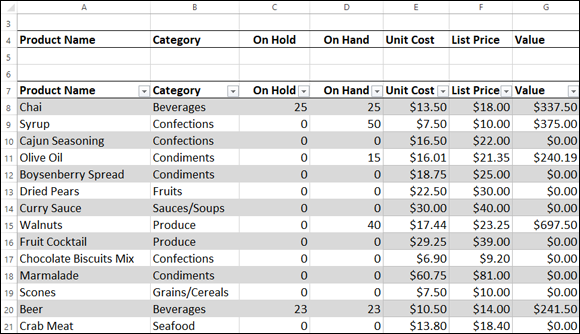
FIGURE 6-1: A table and its criteria range.
Now you can enter your criteria, which consists of one or more comparison expressions that you enter into the cells below the copied header of each column you want to work with:
- Enter the comparison expressions on the same row: This tells Excel to apply the database function to those
fieldrows that match all the comparison expressions you enter. - Enter the comparison expressions on separate rows: This tells Excel to apply the database function to those
fieldrows that match at least one of the comparison expressions you enter.
Retrieving a Value from a Table
As part of your data analysis, retrieving a single value from a table to use in a formula is often useful. For example, if you have a table that lists the inventory of all your products, you might want to check how much of a particular product is on hand now to decide whether now's the time to reorder that product. Similarly, you might want to calculate a product's gross margin given its list price and unit cost:
(List Price – Unit Cost) / List Price
Whenever you need a value from the table to use in a formula, use the DGET function. DGET retrieves a value from a table according to the criteria you specify. The function uses the following syntax:
DGET(database, field, criteria)
For example, consider the Inventory table shown earlier in Figure 6-1. Suppose you want to know how many units are on hand of the product named Beer. To set up the criteria range, you enter Beer below the Product Name field, as shown in Figure 6-2. With that done, you can build your DGET function, which is in cell B1 in Figure 6-2:
DGET(Inventory[#All], "On Hand", A4:G5)
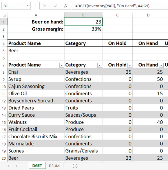
FIGURE 6-2: Use DGET to retrieve a value from a table based on your criteria.
This DGET function is saying to Excel, in effect, “Take a look at the entire table named Inventory, locate the row that has “Beer” in the Product Name column, and then retrieve the value in the On Hand column. Thanks in advance.” Sure enough, DGET returns the value 23 because that's the On Hand value of the Beer product.
Summing a Column's Values
In Chapter 3, “Introducing Excel Tables,” I talk about two ways to display simple table sums: by selecting some column cells and viewing the sum in Excel’s status bar, and by adding subtotals to the table. Those techniques are fine if all you want to do is view the sum, but what if you want to use the sum in a formula or as part of a table summary? Yep, Excel’s SUM function would work, but what if you want the sum of only those items that meet some criteria? For example, in an inventory table, what if you want to know the total value of just the items in the Beverages category?
Ah, for that you need the DSUM function, which adds values from a table based on the criteria you specify. The function uses the standard database function syntax:
DSUM(database, field, criteria)
For example, to get the total value of just the products in the Beverages category, you set up your criteria range with the string Beverages under the Category header (see Figure 6-3). With that value in place, you build your DSUM function (as shown in cell B1 in Figure 6-3):
DSUM(Inventory2[#All], "Value", A3:G4)

FIGURE 6-3: Use DSUM to add a column’s values based on your criteria.
You might be wondering why the table name changed from Inventory in the DGET example to Inventory2 in the DSUM example. That's because in my example workbook for this chapter, I use a separate worksheet for each database function, so when I copy the inventory table to a new worksheet, I need to give the table a new name (because table names must be unique in a workbook).
Counting a Column’s Values
If you select some values in a table column, Excel’s status bar will gladly display a Count item, which tells you how many cells you selected. Fine and dandy, but data analysis is usually a bit more sophisticated than that. For example, in an inventory table, suppose you want to know many products are low in stock (that is, have fewer than 10 in the On Hand column)?
That kind of calculation falls under the bailiwick of both the DCOUNT and DCOUNTA functions, which count records in a table that match criteria you specify:
DCOUNT(database, field, criteria)DCOUNTA(database, field, criteria)
What's the diff? DCOUNT counts the numeric values in field, whereas DCOUNTA counts all the nonblank items in field.
For example, to get the count of the products that have low stock, you set up your criteria range with the expression < 10 under the On Hand header (see Figure 6-4) and then add the DCOUNT function (as shown in cell B1 in Figure 6-4):
DCOUNT(Inventory3[#All], "On Hand", A3:G4)
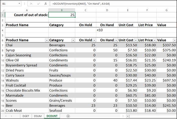
FIGURE 6-4: Use DCOUNT (or DCOUNTA) to tally a column's values based on your criteria.
DCOUNT(Inventory3[#All],, A3:G4)DCOUNTA(Inventory3[#All],, A3:G4)
Note: To omit an argument, leave the space between the two commas empty.
Averaging a Column's Values
The DAVERAGE function calculates an average for values in an Excel list. The unique and truly useful feature of DAVERAGE is that you can specify that you want only table records that meet specified criteria included in your average. DAVERAGE uses the following syntax:
DAVERAGE(database, field, criteria)
As an example of how the DAVERAGE function works, I return to the inventory table and ask a basic question: What’s the average Unit Cost value for those products in the Beverages and Produce categories? To answer this query, you add the text Beverages under the Category header in the criteria range, and then add the text Produce below the Beverages cell, as shown in Figure 6-5. Remember that when you enter criteria using multiple rows, Excel selects those rows in the table that match at least one of the conditions. So, in the example, I'm asking Excel to look for only those products that have either Beverages or Produce in the Category column. Here's the DAVERAGE function that returns the average Unit Cost for those products (see cell B1 in Figure 6-5):
DAVERAGE(Inventory4[#All], "Unit Cost", A3:G5)
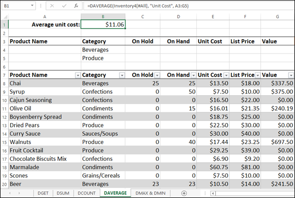
FIGURE 6-5: Use DAVERAGE to average a column’s values based on your criteria.
Notice that I expanded the criteria range to include both rows 4 and 5.
Determining a Column’s Maximum and Minimum Values
Often in data analysis work, looking for outliers is very useful. Outliers are values that are either much greater or much less than the average. One way to check for such anomalous values is to find the largest and smallest values in a column. You can certainly calculate such maxima and minima using every value in the column, but if you’re interested only in those values that meet some criteria, then have I got two functions for you: DMAX and DMIN. These functions find the largest and smallest values, respectively, in a table column for those rows that match the criteria you specify. Both functions use the same standard-issue database function syntax, as shown here:
DMAX(database, field, criteria)
DMIN(database, field, criteria)As an example of how the DMAX and DMIN functions work, suppose you have an inventory table with a Value column that’s the product of the number of units on hand and the unit cost. (For example, a product with 100 units on hand and a $5 unit cost has a total value of $500.) Here’s a question for you: What are the maximum and minimum values for those items in the Produce category that are in stock?
To answer the preceding question, you add the text Produce under the Category header in the criteria range and then add the expression > 0 below the On Hand header, as shown in Figure 6-6. Remember that when you enter multiple conditions on a single row, Excel matches only those rows in the table that match all the conditions. So, in the example, I'm asking Excel to look for only those products that have Produce in the Category column and a value greater than 0 in the On Hand column. Here are the DMAX and DMIN functions that return the maximum and minimum, respectively, for those products (see cells B1 and B2 in Figure 6-6):
DMAX(Inventory5[#All], "Value", A4:G5)DMIN(Inventory5[#All], "Value", A4:G5)
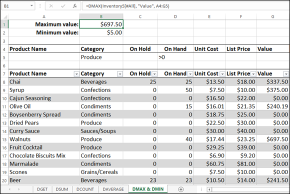
FIGURE 6-6: Use DMAX and DMIN to return a column’s largest and smallest values based on your criteria.
Multiplying a Column’s Values
Lots of table data contains the results of surveys or polls, meaning that the table values are percentages. One way you might want to interrogate such data is to ask, given two percentages, in what percentage are both true in the surveyed population? For example, if your survey says that 50% of people like item A and 50% of people like item B, what percentage of people like both items A and B? You get the answer by multiplying the percentages, so in this case, 25% of the surveyed population like both A and B.
You can perform this kind of table multiplication using the DPRODUCT function, which uses the usual syntax:
DPRODUCT(database, field, criteria)
For example, Figure 6-7 shows the results of a survey that asked people whether they liked certain items. What percentage of people like any two of the items? To calculate this, you set up a criteria range for the Item field and then add the items in separate rows below the Item header. In Figure 6-7, for example, you can see that I added Soggy cereal in the first row and Commuting in the second row. Here's the DPRODUCT function that calculates the answer (see cell B1 in Figure 6-7):
DPRODUCT(A6:B11, 2, A2:A4)
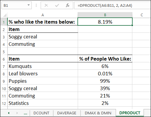
FIGURE 6-7: Use DPRODUCT to multiple a column’s values based on your criteria.
Deriving a Column’s Standard Deviation
One of the most important statistical measures is the standard deviation, which tells you how much the values in a collection vary with respect to the average. I talk about this in more detail in Chapter 11, but for now I can tell you that a low standard deviation means that the data values are grouped near the average, and a high standard deviation means that the values are spread out from the average.
For your table data analysis fun, the DSTDEV and DSTDEVP functions calculate the standard deviation: DSTDEV calculates the standard deviation when you’re working with a sample of the population, whereas DSTDEVP calculates the standard deviation when you’re working with the entire population. As with other database statistical functions, the unique and truly useful feature of DSTDEV and DSTDEVP is that you can specify that you want the calculation to include only those table records that meet your specified criteria.
=DSTDEV(database, field, criteria)=DSTDEVP(database, field, criteria)
For example, in the inventory table, suppose you want to know the standard deviation of the Value column for products in the Condiments category and where the Value column is greater than 0. To set up this calculation, you enter the text Condiments under the criteria range’s Category header and the expression > 10 under the Value header (see Figure 6-8), and then you add the DSTDEV function (as shown in cell B1 in Figure 6-8):
DSTDEV(Inventory6[#All], "Value", A3:G4)
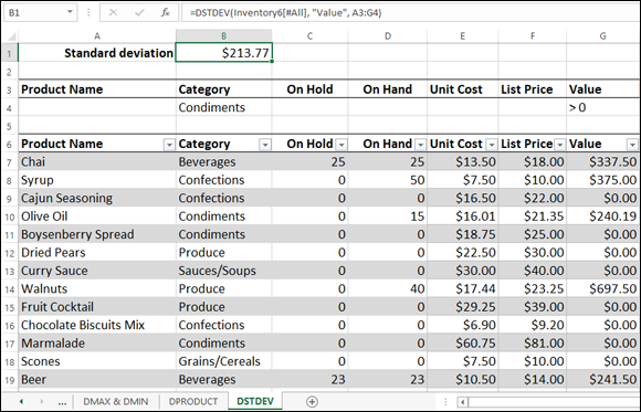
FIGURE 6-8: Use DSTDEV (or DSTDEVP) to derive the standard deviation of a column's values based on your criteria.
Calculating a Column’s Variance
The variance of a set is a measure of how dispersed the data is. The variance is actually the square of the standard deviation, so it’s rarely used because it doesn’t make intuitive sense. (For example, what does it mean to say that a result is in “dollars squared”?)
However, for the sake of completion, I include the fact that Excel does offer the DVAR and DVARP functions to calculate the variance. DVAR calculates the variance when your data is a sample of a larger population, whereas DVARP calculates the variance when your data is the entire population. As with other database statistical functions, using DVAR and DVARP enables you to specify that you want only those table records that meet selection criteria included in your calculations.
The DVAR and DVARP functions use the same syntax:
=DVAR(database, field, criteria)=DVARP(database, field, criteria)
For example, in the inventory table, suppose you want to know the variance of the Unit Cost column for products in the Confections category. To set up this calculation, you enter the text Confections under the criteria range’s Category header (see Figure 6-9) and then add the DVAR function (as shown in cell B1 in Figure 6-8, shown previously):
DVAR(Inventory7[#All], "Unit Cost", A3:G4)
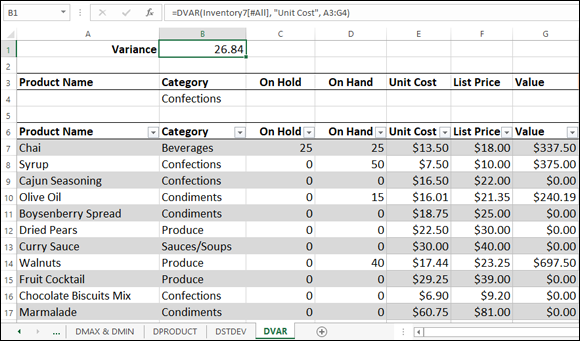
FIGURE 6-9: Use DVAR (or DVARP) to derive the variance of a column’s values based on your criteria.
 By the way, if no record in your list matches your selection criteria, DGET returns the
  The DSTDEV and DSTDEVP functions use the same syntax: