In this chapter, some of the methodological studies are described that were conducted either by means of collateral data collections or by secondary analyses of the core data archives. I begin with a concern that arose following our third cycle: We needed to shift from a sampling-without-replacement paradigm to one that involved sampling with replacement if we were to be able to continue drawing new samples not previously tested (1974 collateral study). I then discuss the issue of the aging of tests and report results from an investigation designed to determine whether switching to more recently constructed tests would be appropriate in the context of the longitudinal study (1975 collateral study). Next, I deal with the question of the effects on participant self-selection when we shifted to the current trend of offering monetary incentives to prospective study participants.
A number of secondary analyses are described that deal with experimental mortality (participant attrition) and the consequent adjustments that might be needed in our substantive findings. Next, I consider the possible effect of repeated measurement designs in understating cognitive decline and present analyses that adjust for practice effects. I then examine the issue of structural equivalence across cohorts, age, time, and gender to determine whether we can validly compare our findings. Here, I describe a number of relevant studies employing restricted (confirmatory) factor analysis designed to determine the degree of invariance of the regression of our observed variables on the latent constructs that are of interest in this study.
The process of maintaining longitudinal panels and supplementing them from random samples of an equivalent population base raises special problems. It has become evident, for example, that over time a sample that is representative of a given population at a study’s inception will become successively less representative. This shift is caused by the effects of nonrandom experimental mortality (participant attrition) as well as by reactivity to repeated testing (practice). The measurement of these effects and possible adjustments for them are discussed later in this chapter. First, however, I consider the effects of circumventing the inherent shortcomings of longitudinal studies by means of appropriate control groups.
One such possible control is to draw independent samples from the same population at different measurement points, thus obtaining measures of performance changes that are not confounded by attrition and practice factors. Such an approach, however, requires adoption of a sampling model that, depending on the size and mobility characteristics of the population sampled, involves sampling either with or without replacement. Sampling without replacement assumes that the population is fixed and large enough so that successive samples will be reasonably equivalent. Sampling with replacement assumes a dynamic population, but one for which on average the characteristics of individuals leaving the population are equivalent to those of individuals replacing them.
Although the independent random sampling approach is a useful tool for controlling effects of experimental mortality, practice, and reactivity, it requires the assumption that the characteristics of the parent population from which sampling over time is to occur will remain relatively stable. Riegel and Riegel (1972, p. 306) argued that such an assumption might be flawed. They suggested, “because of selective death of less able persons (especially at younger age levels) the population from which consecutive age samples are drawn is not homogeneous but, increasingly with age, becomes positively biased.” This argument is indeed relevant for repeated sampling from the same cohorts, but not necessarily for the same age levels measured from successive cohorts. Moreover, successive samples are necessarily measured at different points in time, thus introducing additional time-of-measurement confounds.
Another problem occurs when successive samples are drawn from a population without replacement. Unless the parent population is very large, it will eventually become exhausted. That is, either all members of that population may already be included in the study, or the remainder of the population is either unable or unwilling to participate. In addition, the residue of a limited population, because of nonrandom attrition, may eventually become less and less representative of the originally defined population. As a consequence, at some point in a longitudinal inquiry, it may become necessary to switch from a model of sampling without replacement to one of sampling with replacement.
Subsequent to the third Seattle Longitudinal Study (SLS) cycle, it became clear that a further random sample drawn from the remainder of the 1956 health maintenance organization (HMO) population might be fraught with the problems mentioned above. It therefore became necessary to conduct a special collateral study that would determine the effects of switching to a model of sampling with replacement. We decided to draw a random sample from the redefined population and compare the characteristics of this sample and its performance on our major dependent variables with those of the samples drawn from the original fixed population. This approach would enable us, first, to test whether there would be significant effects and, if so, second, to estimate the magnitude of the differences, which could then be used for appropriate adjustments in comparisons of the later with the earlier data collections (see Gribbin, Schaie, & Stone, 1976).
The original population of the HMO (in 1956) had consisted of approximately 18,000 adults over the age of 22 years. Of these, 2,201 persons had been included in our study through the third SLS cycle. The redefined population base in 1974 consisted of all of the approximately 186,000 adult members regardless of the date of entry into the medical plan (except for those individuals already included in our study). Sampling procedures similar to those described for the main study (see chapter 3) were used to obtain a sample of 591 participants, ranging in age from 22 to 88 years (in 1974).
The membership of the HMO, as of 1956, had been somewhat skewed toward the upper economic levels because many well-educated persons were early HMO joiners for principled rather than economic reasons. The membership was limited at the lower economic levels and almost devoid of minorities. Given these exceptions, the HMO membership did provide a wide range of educational, occupational, and income levels and was a reasonable match of the 1960 and 1970 census figures for the service area. By 1974, however, with the membership grown to 10 times that of the original population, there was a far greater proportion of minorities, as well as a somewhat broader range of socioeconomic levels.
Variables in the collateral study were those included in the first three SLS cycles: the primary mental abilities of Verbal Meaning (V), Spatial Orientation (S), Inductive Reasoning (R), Number (N), and Word Fluency (W) and their composites (Intellectual Ability [IQ] and Educational Aptitude [EQ]); the factor scores from the Test of Behavioral Rigidity (TBR), including Motor-Cognitive Flexibility (MCF), Attitudinal Flexibility (AF), and Psychomotor Speed (PS); and the attitude scale of Social Responsibility (SR) (see chapter 3 for detailed descriptions).
The data collected in the 1974 collateral study can be analyzed by two of the designs derived from the general developmental model (Schaie, 1965, 1977; chapter 2). Assuming that a major proportion of variance is accounted for by cohort-related (year-of-birth) differences, data may be organized into a cross-sequential format— in this instance, comparing individuals from the same birth cohorts, but drawn from two different populations. Alternatively, assuming that age-related differences are of significance, the data can be grouped according to age levels in the form of a time-sequential design—comparing individuals at the same age, but drawn not only from different birth cohorts, but also from different populations. Both designs were used in this study.
Scores for all participants were first transformed into T-scores (M = 50; SD = 10) based on all samples at first test occasion from the first three SLS cycles. For the analyses by cohort, participants in both populations were grouped into 7-year birth cohorts, with mean year of birth ranging from 1889 to 1945. Because the sample from the redefined population was tested in 1974, which was 4 years subsequent to the last measurement point for the original samples, participant groupings were reorganized, and mean year of birth for the new sample was shifted by 4 years to maintain equivalent mean ages for the analyses by age levels. Data were thus available for seven cohorts (mean birth years 1889 to 1945) at all times of measurement. Similarly, data were available for seven age levels (mean ages 25 to 67 years) from all occasions; specifically, observations from Cohorts 1 to 7 in 1956, Cohorts 2 to 8 in 1963, and Cohorts 3 to 9 in 1970 were compared with the reorganized groupings of the participants in the 1974 testing.
Previous analyses of data from the original population samples had suggested a significant time-of-measurement (period) effect (Schaie, Labouvie, & Buech, 1973; Schaie & Labouvie-Vief, 1974). To estimate and control for these effects, trend line analyses were conducted over the first three measurement occasions, and the expected time-of-measurement effect for the 1974 sample was estimated. The coefficients of determination (degree of fit of the linear equation) ranged from .74 to .92 in both cohort and age analyses. Psychomotor Speed and Attitudinal Flexibility in the cohort analysis did not adequately fit a linear mode but could be fitted with a logarithmic function. Estimated values for these variables were therefore obtained subsequent to such transformation. The null hypothesis with respect to the difference between observed scores from the 1974 sample and estimated scores was evaluated by means of independent T-tests.
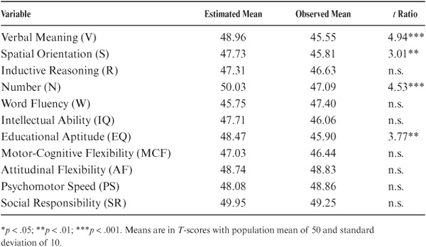
Summary results for the comparison of data from the original and redefined populations can be found in tables 8.1 and 8.2. Significant overall differences (p < .01) between samples from the two populations for both cohort and age analyses were observed on a number of variables: Verbal Meaning, Spatial Orientation, Number, Word Fluency, and the Index of Educational Aptitude. The sample from the redefined population scored somewhat lower than that from the original population, with the exception of Word Fluency, for which it scored higher. No differences were observed for the measures from the Test of Behavioral Rigidity, the Social Responsibility scale, or the composite IQ score.
Having established that differences in level between the two populations did exist on certain variables, the question next arose as to whether these differences prevailed across the board for all cohort/age groups or were localized at specific age levels. This was a critical issue: If there were an overall difference, then future analyses would require systematic adjustments; if the differences were confined to specific age and cohort levels, then we would simply need to take note of this in interpreting local blips in our overall data analyses. Results of the age- and cohort-specific analyses suggested that the differences were indeed local: They affected primarily members of Cohorts 4 and 5 (mean birth years 1910 and 1917, respectively), who in 1974 would have been in their late 50s and early 60s. Comparisons for none of the other age/cohort levels reached statistical significance (p < .01).
TABLE 8.1. Cohort Analysis of Differences Between Estimated and Observed Scores

The major conclusion of this study echoes for the investigation of developmental problems the caution first raised by Campbell and Stanley (1963) that there is always a trade-off between internal and external validity. In our case, we find that designs that maximize internal validity may indeed impair the generalizability of the phenomena studied (see also Schaie, 1978). Fortunately, the results of the 1974 collateral study suggested that such threat to the external validity of developmental designs is not equally serious for all variables or for all ages and cohorts. Hence, I do not necessarily advocate that all studies must include analyses such as the one presented in this section, but I would caution the initiator of long-range studies to design data collections in a manner permitting similar analyses for those variables when the literature does not provide appropriate evidence of external validity.
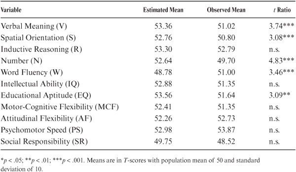
TABLE 8.2. Age Analysis of Differences Between Estimated and Observed Scores
Although longitudinal designs are the most powerful approach for determining changes that occur with increasing age, they are associated with a number of serious limitations (see chapter 2; Baltes & Nesselroade, 1979; Schaie, 1973b, 1977, 1988d, 1994b). One of these limitations is the fact that outmoded measurement instruments must usually continue to be employed, even though newer (and possibly better) instruments may become available, to allow orderly comparisons of the measurement variables over time.
However, if the primary interest is at the level of psychological constructs, then specific measurement operations may be seen as no more than arbitrary samples of observable behaviors designed to measure the latent constructs (Baltes, Nesselroade, Schaie, & LaBouvie, 1972; Schaie, 1973b, 1988d). In this case, it might well be possible to convert from one set of measures to another if the appropriate linkage studies are undertaken. These linkage studies must be designed to give an indication of the common factor structure for both old and new measures.
Designing linkage studies requires considerable attention to a number of issues. New instruments must be chosen that, on either theoretical or empirical grounds, may be expected to measure the same constructs as the old instruments. Thus, it is necessary to include a variety of tasks thought to measure the same constructs. It is then possible to determine empirically which of the new measures best describes information that was gained from the older measures so that scores obtained from the new test battery will closely reproduce the information gathered by the original measures.
The sample of participants for the linkage study must be drawn from the same parent population and should comprise individuals of the same gender and age range as those in the longitudinal study. Only in this manner can we be sure that comparable information will be gathered on the range of performance, reliability, and construct validity for both old and new measures. Given information for the same participants on both the old and new measurement variables, regression techniques can then be employed, the results of which will allow judgment whether to convert to new measures and, if so, which measures must be included in the new battery. Alternatively, study results may suggest that switching to the new measures will result in significant information loss, an outcome that would argue for retention of one or more of the old measures.
Because of the cohort effects described in this volume (see chapter 6), we began to worry as we prepared for the fourth (1977) cycle that a ceiling effect might be reached by some of the younger participants on some of the measures in the 1948 Primary Mental Abilities (PMA) battery. Although these tests have been found to be appropriate for older people (Schaie, Rosenthal, & Perlman, 1953), the question was now raised as to whether the tests had “aged” over the time period they had been used. In other words, we were concerned whether measures retained appropriate construct validity for the more recent cohorts introduced into our study.
On the other hand, we were also concerned about the possibility that, although the test might have restricted validity for the younger cohorts, switching to a newer test might raise construct validity problems for the older cohorts. For example, Gardner and Monge (1975) found that whereas 20- and 30-year-olds performed significantly better on items entering the language after 1960, 40- and 60-year-olds performed significantly better on items entering the language in the late 1920s.
We consequently decided that it would be prudent to examine the continuing utility of the 1948 PMA version by administering this test together with a more recent PMA revision (T. G. Thurstone, 1962) and selected measures from the Kit of Reference Tests for Cognitive Factors published by the Educational Testing Service (ETS; French, Ekstrom, & Price, 1963). The 1962 PMA was chosen because it was felt that this test would be most similar to the 1948 PMA version; the ETS tests were included with the expectation that they might account for additional variance that would reduce the information loss caused by a decision to switch the PMA test for future test occasions (see Gribbin & Schaie, 1977).
The approximately 128,000 members of our HMO over the age range from 22 to 82 years (in 1975) were stratified by age and gender, and a balanced random sample in these strata was drawn. Data were collected on 242 men and women.
The test battery for this study included the five subtests of the PMA 1948 version (Thurstone & Thurstone, 1949): Verbal Meaning (V48), Spatial Orientation (S48), Inductive Reasoning (R48), Number (N48), and Word Fluency (W48). The 1962 version (Thurstone, 1962) differs from the earlier format by omitting Word Fluency; by having Number (N62) include subtraction, multiplication, and division instead of just addition; and by having Inductive Reasoning (R62) include number series and word groupings as well as the letter series that make up N48. The number of items is also increased in the Verbal Meaning (V62) test. Eight tests were added from the ETS test kit (French et al., 1963): Hidden Patterns, a measure of flexibility of closure; Letter Sets, a measure of inductive reasoning; Length Estimation, the ability to judge and compare visually perceived distances; Finding A’s and Identical Pictures, measures of perceptual speed; Nonsense Syllogisms, a measure of syllogistic reasoning; Maze Tracing, which requires spatial scanning; and Paper Folding, which requires transforming the image of spatial patterns into other visual arrangements. All of the ETS tests have two parts of similar form.
Tests were administered in a modified counterbalanced order; that is, one order presented the 1948 PMA first, followed by the ETS tests, with the 1962 PMA last. The second order presented the 1962 PMA first, followed by the ETS tests in reverse order, and ending with the 1948 PMA. A 20-minute break, with refreshments, was given after half the ETS tests had been administered.
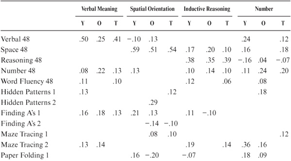
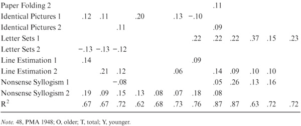
Regression analyses were employed to determine the relationship between the tests. For each subtest score to be predicted (that is, subtests from both versions of the PMA), scores on all subtests from the alternative version plus each part of the eight ETS tests were used as predictor variables across all participants. Because we are also concerned about the relationships among our variables by age level, similar analyses were conducted by dividing the sample into two age groups (22 to 51 and 52 to 82 years) to determine whether predictability of the tests differed by age groupings. Table 8.3 presents the R2 (proportion of variance accounted for each subtest of the 1948 PMA, as well as the β weights (βs, standardized regression coefficients) for each predictor variable for the younger, older, and total data sets. Similar information is provided in table 8.4 for the 1962 PMA.
As can be seen by comparing the R2 of the comparable subtests from each PMA version, it turned out that the 1962 version was better predicted than was the 1948 version. Of the 1948 PMA tests, Verbal Meaning, Spatial Orientation, and Inductive Reasoning could be reasonably well predicted from their 1962 counterparts. However, this was not the case for Number and Word Fluency. For these subtests, only 43% and 40% of the variance, respectively, could be accounted for, suggesting that it would not have been prudent to replace these tests.
When examining findings by age level, it became clear that N48 and W48 were even less well predicted for the younger half of the sample. However, it is worth noting that W48 was better predicted for older than younger participants, and that the reverse finding was true for W62.
These results suggested that, by adding certain of the ETS tests, it would have been practicable to replace V48 with V62, S48 with S62, and R48 with R62 and sustain relatively little information loss. For N48 and W48, however, it was clear that replacement was not justified. By contrast, it was found that a combination of the 1948 PMA and certain of the ETS tests would allow substantial prediction of most of the reliable variance in the 1962 PMA.
In sum, it appeared that shifting to the newer version of the PMA, even with the addition of several other tests, would lead to serious problems in maintaining linkage across test occasions. Moreover, because it was possible to predict performance on the 1962 PMA well with the addition of certain ETS tests, it did not seem that any advantage was to be gained in shifting to the newer test version. We thus concluded that continued use of the 1948 PMA was justified, but we augmented the fourth cycle battery by adding the ETS Identical Pictures and Finding A’s tests to be able to define an additional Perceptual Speed factor.
Over the course of the SLS, there have been a number of subtle changes in the nature of volunteering behavior by prospective participants. In particular, our original solicitation was directed toward encouraging participation by appealing to the prospective participants’ interest in helping to generate new knowledge as well as in assisting their health plan in acquiring information on its membership that might help in program-planning activities. As the study progressed, payments to participants in psychological studies became more frequent, and it is now virtually the rule for study participants beyond college age.
TABLE 8.3. Regression Equations Predicting the 1948 PMA
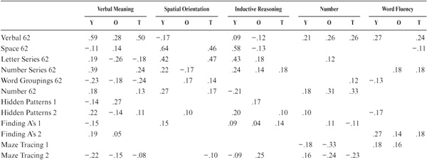

TABLE 8.4. Regression Equations Predicting the 1962 PMA
It has been well known for some time that rate of volunteering differs by age. Typically, adult volunteers tend to be younger, and when older people do volunteer, they tend to so more often for survey research than for laboratory studies (Rosenthal & Rosnow, 1975). Indeed, in our very first effort, we found a curvilinear age pattern, with middle-aged persons most likely to volunteer (Schaie, 1958c).
The increased employment of monetary incentives may have a substantial effect on the self-selection of volunteer study participants. In a study with young adult participants, MacDonald (1972) utilized three incentive conditions: (a) for pay, (b) for extra class credit, and (c) for love of science. He found that participants high in need of approval on the Marlowe-Crowne scale were more willing to volunteer than participants low in need of approval on the pay condition, but not on the other two conditions.
Because we could not find a comparable study using older adults, as part of the 1974 collateral study we attempted to determine the effects of a monetary incentive on self-selection of volunteer participants across the adult age range. Specifically, we were interested in determining whether those participants who had been promised payment differed on certain cognitive and personality factors from those who had been told that they would not be paid (see Gribbin & Schaie, 1976).
Sampling and procedures for this investigation are described in the section on the 1974 collateral study. However, certain additional information relating to the monetary incentive aspects needs to be added. As part of the participant recruitment letter, half of the potential participants were informed that they would be paid $10 for their participation; no mention of payment was made in the letter to the other half. After completion of the assessment procedures, both groups were paid the participant fee. Data evaluated for the effects of monetary incentives included the five primary mental abilities, the TBR, and the 16 PF (16 Personality Factors Test; Cattell, Eber, & Tatsuoka, 1970).
Of the 1,233 potential participants in each incentive category, 34% of the pay condition (P) and 32% of the no-pay condition (NP) participants volunteered to participate in the study. In both conditions, women (P = 37%; NP = 35%) were more willing to participate than men (P = 30%; NP = 29%). Peak participation occurred for participants in the age range from 40 to 68 years, with participation decreasing linearly for both those older and those younger. Nonsignificant chi-squares were obtained for age, gender, and their interaction.
No significant differences for the pay conditions were found for any of the primary mental abilities or any of the dimensions of the TBR. We did not observe any significant pay condition by gender interactions. The effect of incentive conditions on personality traits was next considered via multivariate analyses of variance of both primary source traits and the secondary stratum factors of the 16 PF. Again, none of the multivariate tests of Trait × Pay Condition or Trait × Pay Condition × Gender was statistically significant.
It thus seemed clear that offering a monetary incentive did not seem to result in biased self-selection, at least as far as measures of cognitive abilities, cognitive styles, and self-reported personality traits are concerned. In addition, it did not seem that offering a monetary incentive had any effect on recruitment rate for a relatively brief (2-hour) laboratory experiment. Of course, we do not know whether similar findings would hold for more extensive protocols such as those employed in our training studies (see chapter 7). Nevertheless, it seems safe to argue from these results that findings from studies using monetary incentives may legitimately be generalized to those that do not offer such incentives without fear that the samples will differ regarding characteristics that might be attributed to extraneous incentive conditions.
One of the major threats to the internal validity of a longitudinal study is the occurrence of participant attrition (experimental mortality) such that not all participants tested at T1 are available for retest at T2 or subsequently. In studies of cognitive aging, participant attrition may be caused by death, disability, disappearance, or failure to cooperate with the researcher on a subsequent test occasion.
Substantial differences in base performance have been observed between those who return and those who fail to be retrieved for the second or subsequent test. Typically, dropouts score lower at base on ability variables or describe themselves as possessing less socially desirable traits than do those who return (see Riegel, Riegel, & Meyer, 1967; Schaie, 1988d). Hence, the argument has been advanced that longitudinal studies represent increasingly more elite subsets of the general population and may eventually produce data that are not sufficiently generalizable (see Botwinick, 1977). This proposition can and should be tested empirically, of course. In the SLS, we have assessed experimental mortality subsequent to each cycle (for Cycle 2, see Baltes, Schaie, & Nardi, 1971; Cycle 3, Schaie, Labouvie, & Barrett, 1973; Cycle 4, Gribbin & Schaie, 1979; Cycle 5, Cooney, Schaie, & Willis, 1988; Cycle 6, Schaie, 1996b). Next, I summarize a comprehensive analysis of attrition effects across all seven cycles (see also Schaie, 1988d).
We have examined the magnitude of attrition effects for several longitudinal sequences to contrast base performance of those individuals for whom longitudinal data are available with those who dropped out after the initial assessment. In addition, we considered shifts in direction and magnitude of attrition after multiple assessment occasions.
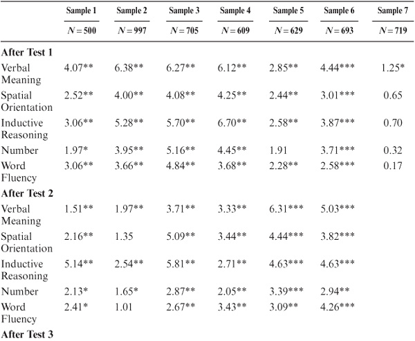
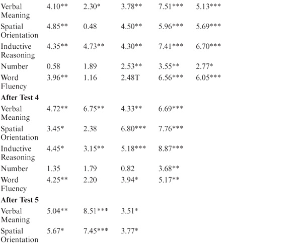
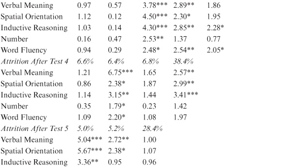
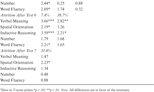
In table 8.5, attrition data are reported as the difference in average performance between the dropouts and returnees. It will be seen that attrition effects vary across samples entering the study at different points in time. However, between T1 and T2, they generally range from 0.3 to 0.6 SD and must therefore be considered of a magnitude that represents at least a moderate-size effect (see Cohen & Cohen, 1975). Although attrition effects become somewhat less pronounced as test occasions multiply, they do remain of a statistically significant magnitude.
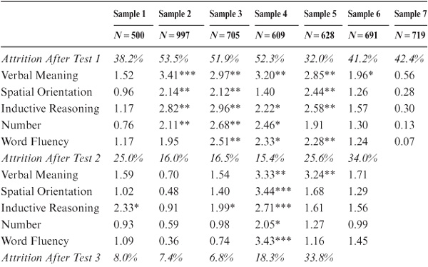
Before the reader is overly impressed by the substantial differences between dropouts and returnees, a caution must be raised. Bias in longitudinal studies because of experimental mortality depends solely on the proportion of dropouts compared with the total sample. Hence, if attrition is modest, experimental mortality effects will be quite small, but if attrition is large, the effects can be as substantial, as noted above. Table 8.6 therefore presents the actual net attrition effects (in T-score points) for our samples, showing the different attrition patterns. It is apparent from these data that experimental mortality is largest for those test occasions when the greatest proportion of dropouts occurred (usually at T2) and becomes smaller as panels stabilized, and the remaining attrition occurred primarily as a consequence of the participants’ death or disability. However, as panels age, the magnitude of experimental mortality may increase again given the often-observed terminal decline occurring prior to death (also see Bosworth, Schaie, & Willis, 1999a; Gerstorf, Ram, Hoppmann, Willis, & Schaie, 2011).
TABLE 8.5. Difference in Average Performance at Base Assessment Between Dropouts and Returnees
We can infer from these data that parameter estimates of levels of cognitive function from longitudinal studies, when experimental mortality is appreciable, could be substantially higher in many instances than would be true if the entire original sample could have been followed over time. Nevertheless, it does not follow that rates of change will also be overestimated unless it can be shown that there is a substantial positive correlation between base level performance and age change. Because of the favorable attrition (i.e., excess attrition of low-performing participants), the regression should result in modest negative correlations between base and age change measures. This is indeed what was found (see Schaie, 1988d, 1996b). Hence, contrary to Botwinick’s (1977) inference, experimental mortality may actually result in the overestimation of rates of cognitive aging in longitudinal studies.
Longitudinal studies have been thought to reflect overly optimistic results also because age-related declines in behavior may be obscured by the consequences of practice on the measurement instruments used to detect such decline. In addition, practice effects may differ by age. We have studied the effects of practice by comparing the performance of individuals who return for follow-up with the performance of individuals assessed at the same age for the first time (Schaie, 1988d).
TABLE 8.6. Attrition Effects Calculated as Difference Between Base Means for Total Sample and Returneesa
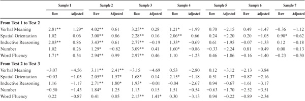
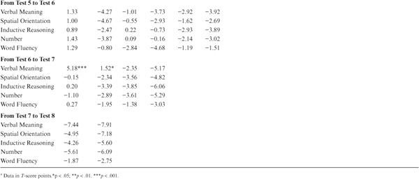
Practice effects estimated in this manner appear, at first glance, to be impressively large between T1 and T2 (up to approximately 0.4 SD), although they become increasingly smaller over subsequent time intervals (see table 8.7). The exceptions involve Verbal Meaning and Word Fluency, for which practice effects are again noted late in life. Note, however, that practice effects estimated in this manner of necessity involve the comparison of attrited and random samples. The mean values for the longitudinal samples must therefore be adjusted for experimental mortality to permit valid comparison. The appropriate adjustment is based on the values in table 8.6 (i.e., the differences between returnees and the entire sample). Because practice effects are assumed to be positive, all significance tests in table 8.7 were one tailed. Although the raw practice effects appear to be significant for most variables and samples, none of the adjusted effects reached significance except for Verbal Meaning in Sample 1 from T1 to T2 and from T6 to T7. We concluded, therefore, that practice effects do not tend to produce favorably biased results in the longitudinal findings of our study.
We have also examined the joint effects of attrition and history, attrition and cohort, history and practice, cohort and practice, and the joint effects of all these four potential threats to the internal validity of longitudinal studies. Designs for these analyses have been provided (Schaie, 1977), with worked-out examples in Schaie (1988d). In a data set involving two age cohorts aged 46 and 53 years at the first assessment and comparing their performance 7 years later, these effects were all significant and accounted for roughly 7% of the total variance (see Schaie, 1988d, for further details).
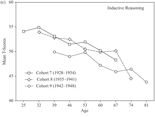
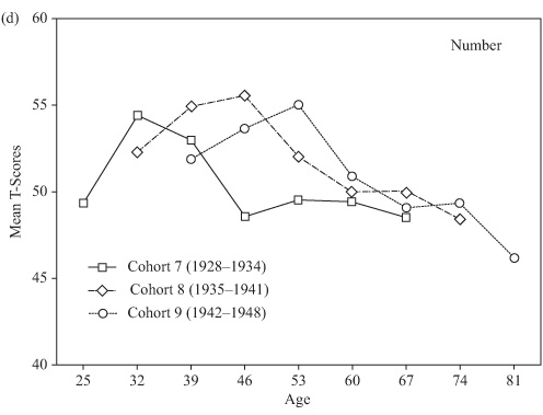
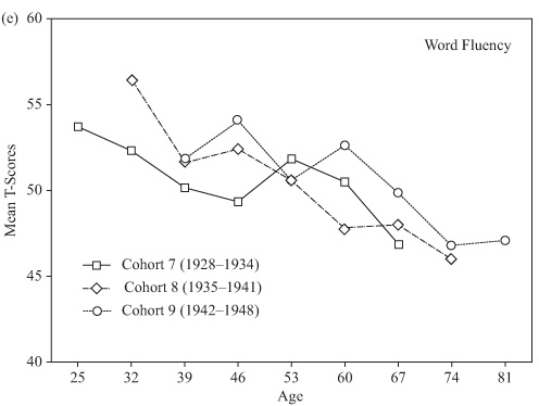
As indicated in chapter 2, it is possible to control for the effects of practice and attrition by examining a longitudinal sequence or sequences that use only the first-time data of random samples drawn from the same cohort at successive ages. Such a design, of course, requires a population frame with average membership characteristics that remain rather stable over time. Given the seven waves of data collections in the SLS, data are now available over a 42-year range for three of our study cohorts (Cohorts 7–9). It is therefore possible to construct age gradients over the age range from 25 to 81 years of age that would be controlled for effects of attrition and practice.
These gradients are obtained from table 4.2 (see chapter 4, “Cross-Sectional Studies”), by taking the averages at each successive age from the sample entering the study at that age for the first time. Figures 8.1a through 8.1e show the results of these analyses for the five basic primary mental abilities. Although these data cannot be used to predict changes within individuals, they provide conservative bottom-line estimates of what the population parameters would likely be in the absence of attrition and practice effects. It should be noted that there are substantial cohort differences in these sequences. More stable estimates would require extending the sequence over additional cohorts.
TABLE 8.7. Raw and Attrition-Adjusted Effects of Practice by Sample and Test Occasiona

I suggest in chapter 2 that all of the comparisons across age and time as well as the gains reported for cognitive interventions depend on the assumption that structural invariance is maintained across these conditions. Very few studies have the requisite data to investigate this assumption empirically. In this section, I describe four methodological investigations that applied restricted (confirmatory) factor analysis (Mulaik, 1972) to investigate these issues. All of the analyses use the linear structural relations (LISREL) paradigm (Jöreskog & Sörbom, 1988).
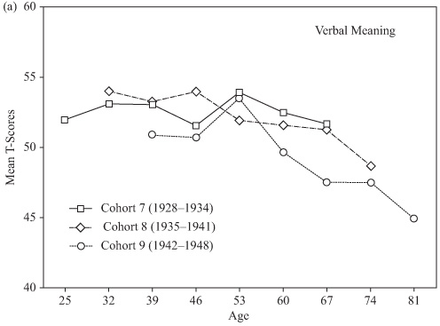
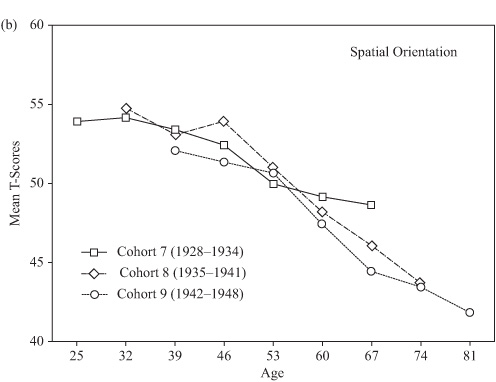
FIGURE 8.1. Longitudinal age gradients obtained from independent random samples controlling for effects of attrition and practice.
In a study employing the entire set of 1,621 participants tested in 1984, we investigated the validity of the assumption that the measurement operations employed in the study are comparable across age groups (Schaie, Willis, & Chipuer, 1989). The basic assumption to be tested was that each observed marker variable measures the same latent construct equally well regardless of the age of the participants assessed.
Three levels of stringency of measurement equivalence were defined: strong metric invariance, weak metric invariance, and configural invariance (see also Bentler, 1980; Horn, 1991; Horn & McArdle, 1992; Meredith, 1993; Schaie, 2000d). The most stringent level of invariance, strong metric invariance, implies not only that the measurement operations remain relevant to the same latent construct, but also that the regressions of the latent constructs on the observed measures remain invariant across age and further that the interrelationships among the different constructs representing a domain (factor intercorrelations) also remain invariant. If invariance can be accepted at this level, then it follows that inferences can be validly drawn from age-comparative studies both for the comparison of directly observed mean levels and for the comparison of derived factor score means for the latent ability constructs.
A somewhat less stringent equivalence requirement, weak metric invariance, allows the unique variances and factor intercorrelations to vary across groups while requiring the regressions of the latent constructs on the observed variables to remain invariant. Given the acceptability of this relaxed requirement, it is still possible to claim that observations remain invariant across age. However, comparison of factor scores now requires that changes in the factor space (unequal factor variances and covariances) should be adequately modeled in the algorithm employed for the computation of factor scores.
For the least stringent requirement, configural invariance, we expect that the observable markers of the constructs remain relevant to the same latent construct across age (i.e., across age groups, the same variables have statistically significant loadings, and the same variables have zero loadings). However, we do not insist that the relationships among the latent constructs retain the same magnitude, and we do not require that the regression of the latent constructs on the observed variables remain invariant. If we must accept the least restrictive model, we must then conclude that our test battery does not measure the latent constructs equally well over the entire age range studied, and we must estimate factor scores using differential weights by age group.
In this analysis, we tested the hypothesis of invariance under the three assumptions outlined above for the domain of psychometric intelligence as defined by 20 tests representing multiple markers of the latent constructs of Inductive Reasoning, Spatial Orientation, Perceptual Speed, Numeric Ability, and Verbal Ability (see description of the expanded battery in chapter 3. An initial factor structure (suggested by earlier work described below [see also Alwin 1988; Alwin & Jackson, 1981; Schaie, Willis, Hertzog, & Schulenberg, 1987]) was confirmed on the entire sample’s 1,621 study participants, yielding a satisfactory fit [χ2 (107, N = 1621) = 946.62, p < .001 (goodness-of-fit index [GFI] = .936)]. Table 8.8 shows the factor loadings and factor intercorrelations that entered subsequent analyses. In this model, each ability is marked by at least three operationally distinct observed markers. Each individual test marks only one ability, except for Number Comparison, which splits between Perceptual Speed and Number, and the PMA Verbal Meaning test, which splits between Perceptual Speed and Verbal Comprehension.
The total sample was then subdivided by age into nine nonoverlapping subsets with mean ages 90 (n = 39), 81 (n = 136), 74 (n = 260), 67 (n = 291), 60 (n = 260), 53 (n = 193), 46 (n = 154), 39 (n = 124), and 29 (n = 164) years. The variance–covariance matrix for each set was then modeled with respect to each of the three invariance levels specified for the overall model.
As indicated in this section, model testing then proceeded at the three levels of stringency listed for determining factorial invariance:
1. Strong metric invariance. Model fits for the subsets were, of course, somewhat lower than for the total set, but except for ages 81 and 90 years (the oldest cohorts), they were still quite acceptable. The oldest cohort, perhaps because of the small sample size, had the lowest GFI (.596), and the 67-year-olds had the highest (.893).
2. Weak metric invariance. When unique variances and the factor variance–covariance matrices were freely estimated across groups, statistically significant improvements of model fit occurred for all age groups. As in the complete metric invariance models, the poorest fit (.669) was again found for the oldest age group, with the best fit (.913) occurring for the 74-year-olds. Substantial differences in factor variances were found across the age groups. Variances increased systematically until the 60s and then decreased. Covariances also showed substantial increment with increasing age.
3. Configural invariance. In the final set of analyses, factor patterns as specified in table 8.8 were maintained, but the factor patterns were freely estimated. Again, significant improvement in fit was obtained for all age groups, with the goodness-of-fit indices ranging from a low of .697 for the oldest group to a high of .930 for the 74-year-olds. Hence, the configural invariance model must be accepted as the most plausible description of the structure of this data set.
TABLE 8.8. Measurement Model for the 1984 Data Set
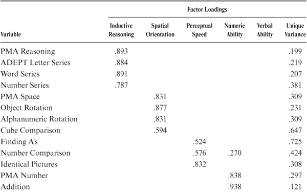
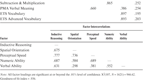
The demonstration of configural (factor pattern) invariance is initially reassuring to developmentalists in that it confirms the hope that it is realistic to track the same basic constructs across age and cohorts in adulthood. Nevertheless, these findings give rise to serious cautions with respect to the adequacy of the construct equivalence of an age-comparative study. Given the fact that we could not accept a total-population-based measurement model at either metric or incomplete metric invariance level for any age/cohort, we had to consider the use of single estimators of latent constructs as problematic in age-comparative studies.
How serious is the divergence from complete metric equivalence? In the past, shifts in the interrelation among ability constructs have been associated with a differentiation-dedifferentiation theory of intelligence (see Reinert, 1970; Werner, 1948). This theory predicts that factor covariances should be lowest for the young and should increase with advancing age. As predicted by theory, we found factor covariances were lowest for our youngest age groups and increased with advancing age. Factor variances also increased until the 70s, when the disproportionate dropout of those at greatest risk again increased sample homogeneity and reduced factor variances. Because our data set for the test of complete metric invariance was centered in late midlife, it does not surprise us that discrepancies in factor covariances were confined primarily to the extremes of the age range studied (see Schaie et al., 1989). Consequently, these shifts will not seriously impair the validity of age comparisons using factor scores except at the age extremes.
Because we accept the configural invariance model as the most plausible description of our data, we must be concerned about the relative efficiency of the observed variables as markers of the latent variables at different age levels. The shift in efficiency may be a function of the influence of extreme outliers in small samples or a consequence of the attainment of floor effects in the older age groups and ceiling effects in the younger age groups when a common measurement battery is used over the entire adult life course. In this study, across age groups, for example, the Cube Comparison test becomes a less efficient marker of Spatial Orientation, whereas the PMA Space test becomes a better marker with increasing age. Likewise, the Number Comparison test (a marker of Perceptual Speed), which has a secondary loading on Numerical Ability in the general factor model, loses that secondary loading with increasing age.
These findings suggested that age comparisons in performance level on certain single markers of a given ability might be confounded by the changing efficiency of the marker in making the desired assessment. Fortunately, in our case, the divergences are typically quite local in nature. That is, for a particular ability, the optimal regression weights of observable measures on their latent factors may shift slightly, but because there is no shift in the primary loading to another factor, structural relationships are well maintained across the entire age range sampled in the study.
We have also investigated the stability of the expanded battery’s ability structure across the cognitive training intervention described in chapter 7 (Schaie et al., 1987). This study was designed to show that the structure of abilities remains invariant across a brief time period for a nonintervention group (experimental control) and to show that the two intervention programs (Inductive Reasoning, Spatial Orientation) employed in the cognitive intervention study did not result in shifts of factor structure, a possible outcome for training studies suggested by Donaldson (1981; but see Willis & Baltes, 1981).
The subset of participants used for this study included 401 persons (224 women and 177 men) who were tested twice in 1983–1984. Of these, 111 participants received Inductive Reasoning training, 118 were trained on Spatial Orientation, and 172 were pre- and posttested but did not receive any training. Mean age of the total sample in these analyses was 72.5 years (SD = 6.41, range = 64–95 years). Mean educational level was 13.9 years (SD = 2.98; range = 6–20 years). The test battery consisted of 16 tests representing multiple markers of the latent constructs of Inductive Reasoning, Spatial Orientation, Perceptual Speed, Numeric Ability, and Verbal Ability (see description of the expanded battery in chapter 2).
We first used the pretest data for the entire sample to select an appropriate factor model. Given that the training analysis classified groups by prior developmental history, we next evaluated the metric invariance of the ability factor structure across the stable and decline groups (see chapter 7). Both groups had equivalent factor loadings and factor intercorrelations [χ3(243, N = 401) = 463.17; GFI stable = .847, GFI unstable = .892]. A similar analysis confirmed the acceptability of metric invariance across gender [χ2(243, N = 401) = 466.22; GFI men = .851, GFI women = .904]. Finally, metric invariance could be accepted also across the three training conditions [X2(243, N = 401) = 511.55; GFI Inductive Reasoning = .871, GFI Spatial Orientation = .783, controls = .902].
In the main analysis, separate longitudinal factor analyses of the pretest–post-test data were run for each of the training groups. The basic model extended the five-factor model for the pretest data to a repeated measures factor model for the pretest–posttest data. The model also specified correlated residuals to allow test-specific relations across times to provide unbiased estimates of individual differences in the factors (see Hertzog & Schaie, 1986; Sörbom, 1975).
Examination of the pretest–posttest factor analysis results for the control group led to the acceptance of metric invariance with an adequate model fit [χ2N = 172) = 574.84; GFI = .833]. Freeing parameters across test occasions did not lead to a significant improvement in fit, thus indicating short-term stability of factor structure and providing a benchmark for the pretest–posttest comparisons of the experimental intervention groups.
The fit of the basic longitudinal factor model for the Inductive Reasoning training group was almost as good as for the controls [χ2(412, N = 111) = 599.00; GFI = .767]. It appeared that most of the difference in model fit could be attributed to subtle shifts in the relative value of factor loadings among the Inductive Reasoning markers; specifically, after training, the Word Series test received a significantly lower loading, whereas the Letter and Number Series tests received higher loadings.
The Spatial Orientation training group had a somewhat lower model fit across occasions [χ2(411, N = 118) = 700.84; GFI = .742]. Again, the reduction in fit was a function of slight changes in factor loading for the markers of the trained ability, with increases in loadings for PMA Space and Alphanumeric Rotation and decrease in the loading for Object Rotation.
In both training groups, the integrity of the trained factor with respect to the other (nontrained) factors remained undisturbed. Indeed, the stability of individual differences on the latent constructs remained extremely high, with the correlations of latent variables from pretest to posttest in excess of .93.
In this study, we first demonstrated that our measurement model for assessing psychometric ability in older adults remained invariant across gender and across subsets of individuals who had remained stable or declined over time. We next demonstrated short-term stability of factor structure (that is, impermeability to practice effects) by demonstrating strong metric invariance of factor structure for a control group. We also demonstrated high stability of the estimates of the latent constructs across test occasions.
The hypothesis of factorial integrity across experimental interventions was next tested separately for the two training groups. In each case, configural invariance was readily demonstrated. However, in each case some improvement of model fit could be obtained by allowing for shifts in the factor loadings for one of the markers of the trained ability. Nevertheless, the stability of the latent constructs also remained above .93 for the trained constructs. Perturbations in the projection of the observed variables on the latent ability factors induced by training were specific to the ability trained, were of small magnitude, and had no significant effect with respect to the relationship between the latent constructs and observed measures for the nontrained abilities. Hence, we provided support to the construct validity for both observed markers and estimates of latent variables in the training studies reported in chapter 7.
The 1991 data collection provided us with complete repeated measurement data on the expanded battery for 984 study participants. These data were therefore used to conduct longitudinal factor analyses within samples across time. We consequently present data on the issue of longitudinal invariance over 7 years for the total sample as well as six age/cohort groups: ages 32 to 39 (n = 170), 46 to 53 (n = 128), 53 to 60 (n = 147), 60 to 67 (n = 183), 67 to 74 (n = 194), and 76 to 83 (n = 162) years (see also Schaie, Maitland, & Intrieri, 1998).
We first established a baseline model (M1) that showed factor pattern invariance across time and cohort groups, the minimal condition necessary for any comparisons whether they involve cross-sectional or longitudinal data. In this, as in subsequent analyses, the factor variance–covariance matrices (psi) and the unique variances (theta epsilon) are allowed to be estimated freely across time and groups. The model differs from that described above (pp. xxx, also cf. Schaie et al., 1991) by setting the Word Fluency parameter on Verbal Recall to zero and by adding a gender factor that allows salient loadings for all variables. Given the complexity of this data set, this model showed a reasonably good fit: χ2(3,888, N = 982) = 5155.71, p < .001 (GFI = .81; Z ratio = 1.33).
Four weak factorial invariance models were tested; the first two were nested in M1. The first model (M2) constrained the factor loadings (lambda) equal across time. This is the critical test for the invariance of factor loading within a longitudinal data set. This model resulted in a slight but statistically nonsignificant reduction in fit: χ2(3,990, N = 982) = 5288.98, p < .001 (GFI = .81; Z ratio = 1.33); ΔX2(102) = 133.27, p > .01. Hence, we concluded that factorial invariance within groups across time could be accepted.
A second model (M3) allowed the values of the factor loadings (lambda) to be free across time, but constrained equally across cohort groups. This is the test of factorial invariance for the replicated cross-sectional comparisons across cohorts. The model showed a highly significant reduction in fit compared with M1: χ2(4,258, N = 982) = 5790.65, p < .001 (GFI = .78; Z ratio = 1.36); ΔX2(370) = 634.94, p < .001. As a consequence, this model had to be rejected, and we concluded that there are significant differences in factor loadings across cohorts.
The third model (M4), which is nested in both M2 and M3, constrains the factor loadings (lambda) equally across time and group. This particular model, if accepted, would demonstrate factorial invariance both within and across groups. The fit for this model was χ2(4,275, N = 982) = 5801.09, p < .001 (GFI = .78; Z ratio = 1.36). The reduction in fit was significant in the comparison with M2, ΔX2(285) = 512.11, p < .001, but not significant when compared with M3, ΔX2(17) = 10.44, p > .01. The test of this model provides further confirmation that we can accept time invariance within cohorts but cannot accept invariance across cohort groups.
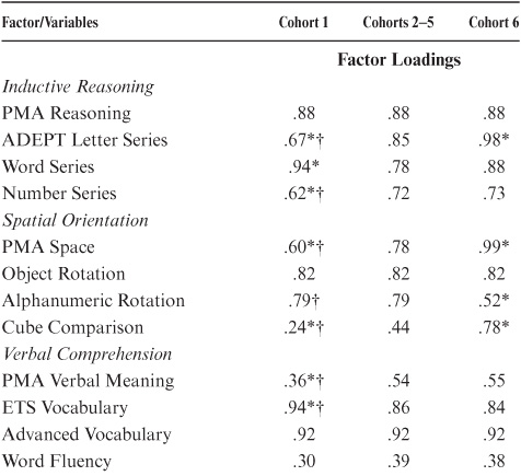
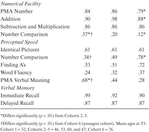
Before totally rejecting factorial invariance across all cohorts, we also tested a partial invariance model (cf. Byrne, Shavelson, & Muthén, 1989) that constrains factor loadings across time and constrains factor loadings across all but the youngest and oldest cohorts (M5). We arrived at this model by examining confidence intervals around individual factors, χ2(4,161, N = 982) = 5484.20, p < .001 [GFI = .81; Z ratio = 1.30, X2(171) = 195.22, p < .09]. Hence, we concluded that this model can be accepted, and that we had demonstrated partial invariance across cohorts. Because we accepted model M5 (invariance across time and partial invariance across groups), we report time-invariant factor loadings separately for Cohorts 1 and 6, as well as a set of loadings for Cohorts 2 to 5 in table 8.9.
When differences in factor loadings between cohorts are examined, it is found that the significant cohort differences are quite localized. No significant differences were found on the Verbal Recall factor. Significant differences on Inductive Reasoning were found for all markers except PMA Reasoning. Significant differences on Spatial Orientation were found for all but the Object Rotation test. Loadings increased with age for Alphanumeric Rotation but decreased for Cube Comparison. On Perceptual Speed, loadings for Number Comparison decreased and loadings on Verbal Meaning increased with age. The loading of Verbal Meaning on the Verbal Comprehension factor, in contrast, decreased with age. Finally, there was a significant increase for the loadings of Number Comparison on the Numerical Facility factor.
TABLE 8.9. Rescaled Solution for Multigroup Analyses
An interesting question long debated in the developmental psychology literature is whether differentiation of ability structure occurs in childhood and adolescence and is followed by dedifferentiation of that structure in old age (see Reinert, 1970; Werner, 1948; also see Schaie, 2000d, for details on using restricted factor analysis to test the hypothesis).
As with the tests of measurement models described in this chapter, we first added the time constraint for the factor variance–covariance matrices to our accepted measurement model (M5). The fit of this model (M6) was χ2(4,287, N = 982) = 5642.74, p < .001 (GFI = .80; Z ratio = 1.32). The reduction in fit in the comparison with M5 was not significant [Δχ2(126) = 158.51, p < .033]. Hence, we concluded that this model can be accepted, and that we failed to confirm dedifferentiation over a 7-year time period.
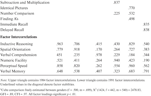
Consistent with our earlier strategy in considering partial invariance models, we also tested the analogy of M5 for the variance–covariance differences. That is, we constrained the psi matrices across time and for Cohorts 2 to 5 but allowed the psis for Cohorts 1 and 6 to differ. The fit of this model (M7) was χ2(4,535, N = 982) = 5938.53, p < .001 (GFI = .79; Z ratio = 1.31). This model is nested in M6. The reduction in fit in the comparison with M9 was significant, ΔX2(248) = 295.79, p < .01. This model cannot be accepted, and we concluded that there were significant differences in the factor intercorrelations across some, but not all, cohorts. Table 8.10 provides the factor intercorrelations for the accepted model.
Our findings on changes in covariance structures from young adulthood to old age lend at least partial support for the differentiation-dedifferentiation theory (figure 8.2). I show magnitudes of intercorrelations for the 1984 and 1991 test occasions for a young adult cohort at ages 29 and 36 years and an old adult cohort at ages 76 and 84 years. Note that factor intercorrelations decreased slightly for 11 of 15 correlations for the young cohort, but increased for all correlations for the old cohort.
The 1991 and 1998 data sets described above were further examined to assess the invariance of factor structures across gender and time at various ages (Maitland, Intrieri, Schaie, & Willis, 2000). For this analysis, the subsets were younger adults (mean age 35.5 years, range 22–49 years; n = 296; 134 men, 162 women); middle-aged adults (mean age 56.5 years, range 50–63 years; n = 330; 154 men, 202 women); and older adults (mean age 75.5 years, range 64–87; n = 356; 154 men, 176 women).
Again, three models were considered. The first tested the hypothesis of time invariance of factor loadings. Next, gender invariance of the factor loadings was tested. Finally, a simultaneous test of invariance between genders and across time was examined.
The configural invariance model (M1), allowed factor loadings to be estimated freely for both gender and occasion [χ2 = 2328.81(1,296), p < .001, GFI = 894, comparative fit index (CFI) = .975]. Model M2 tested invariance across time and constraining factor loadings across occasion and estimated loadings separately for men and women [X2 = 2371.03(1330), p < .001, GFI = .892, CFI =.975; ΔX2 = 42.21(34), p > .16]. The time invariance model did not differ significantly from the configural model. Hence, we accepted the hypothesis of time invariance of factor loadings within gender groups. Model M3 estimated the factor loadings freely across occasion and tested the hypothesis of gender invariance of factor loadings [X2 = 2396.18 (1330), p < .001, GFI = .890, CFI = .974; ΔX2 = 67.36(34), p < .001]. The ΔX2 was significant, and we therefore rejected the hypothesis of gender invariance.
Because time invariance was accepted and gender invariance was not, we evaluated individual gender constraints for all cognitive tests at both time points. The only significant gender difference noted for the 20 cognitive tests was for the Cube Comparison task at T1 (z = −4.88) and at T2 (z = −3.78). Therefore, relaxing the equality constraint for the Cube Comparison test between genders, at both time points, provided our test of partial measurement invariance (M4). This model was compared to the configural measurement model (M1) and had an acceptable fit [χ2 = 2373.13 (1328), p < 0.001, GFI = .892, CFI = .974; ΔX2 = 44.32 (32), p > .07].
TABLE 8.10. Factor Intercorrelations and Stabilities for Cohort Groups
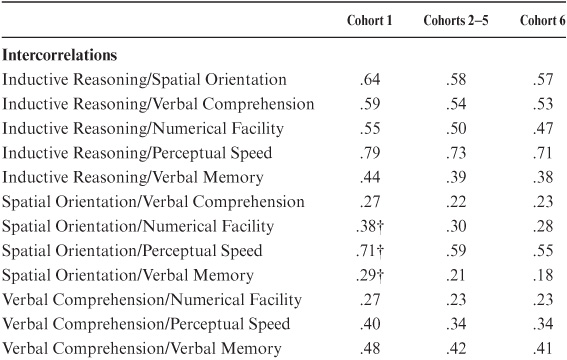
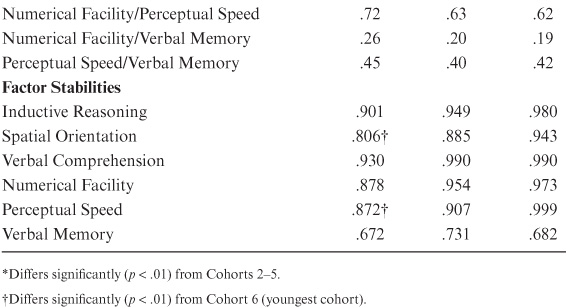
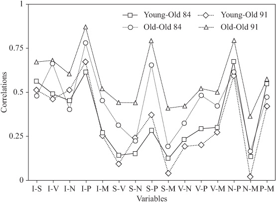
FIGURE 8.2. Correlations among the latent ability constructs across time for the youngest and oldest cohorts.
Once we were able to accept the partially invariant model, we could next add the longitudinal equivalence of factor loadings. This partially invariant model (M5) tested the hypothesis of simultaneous invariance of factor loadings between genders and across time [χ2 = 2390.97 (1346), p < .001, GFI = .891, CFI = .974; ΔX2 = 62.16 (50), p > .12]. This model did not differ significantly and could therefore be accepted; it proved to be the most parsimonious solution (i.e., gender and time invariance for all loadings for the cognitive tasks across 7 years with the exception of gender differences in the Cube Comparison task). Factor loadings and factor correlations for the accepted model may be found in table 8.11.
As we expected from the earlier cross-sectional analyses, we could accept invariance of factor patterns, but not of the regression coefficients, across age/cohort groups or across gender. However, gender invariance was restricted to a single cognitive task, and cohort differences were confined primarily to the youngest and oldest cohorts. Within groups, we could accept the stability of the regression weights across time at least over 7 years. These findings strongly suggested greater stability of individual differences within cohorts than across cohorts or gender, and they provided further arguments for the advantages of acquiring longitudinal data sets.
This chapter describes some of the methodological studies conducted by secondary analyses of the core data archives or through collateral data collections. The first study examined the consequences of shifting from a sampling-without-replacement paradigm to one that involved sampling with replacement. I concluded that no substantial differences in findings result; hence, the first three data collections using the sampling-without-replacement approach are directly comparable to later studies using the sampling-with-replacement paradigm. The second study investigated the “aging” of tests by comparing the 1949 and 1962 PMA tests. It concluded that there was advantage in retaining the original measures. The third study considered the question of shifts in participant self-selection when changing from a non-paid to a paid volunteer sample. No selection effects related to participant fees were observed.
A set of secondary analyses is described that dealt with the topic of experimental mortality (participant attrition) and the consequent adjustments needed for our substantive findings. Such adjustments primarily affect level of performance, but not the rate of cognitive aging. Analyses of the effect of practice occurring when the same variables are administered repeatedly showed only slight effects over 7-year intervals, but methods are presented for adjusting for the observed practice effects.
TABLE 8.11. Standardized Factor Loadings and Factor Correlations for the Accepted Partial Invariance Gender Model

Finally, I consider the issue of structural invariance of the psychometric abilities across cohorts, gender, age, and time. Findings are presented from analyses using restricted (confirmatory) factor analysis to determine the degree of invariance of the regression of the observed variables on the latent constructs of interest in this study. Cross-sectional factor analyses resulted in a demonstration of configural (pattern) invariance, but not of strong metric invariance. These findings implied that factor regressions for young adults and the very old may require differential weighting in age-comparative studies. Another study demonstrated factorial invariance across a cognitive training intervention, confirming that cognitive training results in quantitative change in performance without qualitative shifts in factor structure. Last, I report on longitudinal factor analyses that suggested significant shifts in the variance–covariance matrices, but stability of regression coefficients linking the observed variables and latent constructs over a 7-year period. This study has also examined gender equivalence in structure, which was confirmed except for one of our cognitive tasks (Cube Comparison).