The systemic-risk misperceptions leading up to the current economic malaise evolved over more than three decades and accelerated during the last decade. This chapter presents the history of economic “paradoxes” associated with recent misperceptions. That history is presented in chronological order. Explaining what happened after the fact, and then saying you knew it all along, is always easier than at the time. This chapter avoids the appearance of such retrospective claims by using only the data available at the time and the results published in peer reviewed journals during each of the time periods considered, with new results left for the end of the chapter.
The origins of the economy’s current problems began to evolve in the 1960s and 1970s. That was a time period of unusual diversity, controversy, and dissent within the economics profession. Previously the profession was divided between those economists who advocated use of mathematics in economic theory, and those who opposed it. The economists who opposed it were divided between two groups: (1) those who advocated use of scientific methodology, but applying graphical techniques with minimal use of mathematics, and (2) those “institutionalists,” who advocated a literary, liberal-arts approach to economics, resembling what now is sometimes called “postmodernism” or “deconstructionism.” A leading figure among the institutionalists was Clarence Ayers at the University of Texas. Although he was a professor in the Economics Department, his PhD was in philosophy and his books read more like philosophy books than like modern economics books. By the time that the 1970s arrived, the value of mathematics in economics had become well established, and institutionalism was in a decline. But a new source of debate had arisen: the division between Keynesianism and monetarism, the latter of which was increasing in influence.
This section describes the earliest sources of the misperceptions about systemic risk, with emphasis on the year 1974, during which mysterious structural shifts were purported to have occurred within the American economy. Those shifts were often imputed to “missing money” and to other such phenomena outside the normal domain of the field of economics. Using a reputable measure of money based on state-of-the-art aggregation theory, I found no evidence of structural shifts and showed, with my coauthors, that the misperceptions at that time were caused by defective Fed data. The source of the results in this section, along with further details, can be found in Barnett, Offenbacher, and Spindt (1984) and Barnett (1982). As seen in subsequent sections below, these matters have been growing in importance, as asset substitution and financial innovation have progressed over time.
Demand and supply of money were fundamental to macroeconomics and to central bank policy until the 1970s, when questions began to arise about the stability of monetary demand and supply. In economic theory, microeconomics commonly determines relative prices, while the demand and supply for money determines the price level. But something was believed to have gone wrong in the 1970s. Central to the demand for money was the concept of monetary circulation “velocity,” defined to be national income divided by the supply of money. According to the relevant theory, people are willing to hold a lot of cash and keep a lot of money in checking accounts, when the interest rates paid on alternative uses of money are low. But when interest rates increase, holding a lot of cash or checking account deposits foregoes the high interest rate that could have been received on alternative investments. As a result, cash and demand deposits are managed more aggressively to keep their balances low. Money passes from person to person more rapidly, increasing the turnover rate of money, and thereby monetary velocity. Interest is paid on assets as compensation for giving up monetary services. In short, with any valid definition of money, velocity of circulation should rise and fall with interest rates.
During the 1970s the relevant theory about the properties of the demand for money were widely viewed to have failed. The relationship between the demand for money and interest rates was presumed to have been reversed throughout that decade. In 1974 the demand and supply for money were viewed as having shifted without economic explanation, and a large amount of money was viewed as having disappeared in the “missing money” paradox. At the time I called all of those puzzles the “space alien theories,” since they argued that what happened had no explanation on this planet.
Figure 3.1
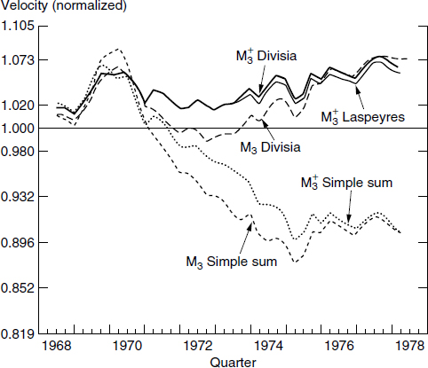
Seasonally adjusted normalized velocity during the 1970s
Now look at figure 3.1 and observe the behavior of the velocity of the FRB staff’s aggregates, M3 and M3+ (later called L).1 Based on the findings of Barnett (1982), those two broad aggregates were chosen to explore the demand for money puzzles in the 1970s. Also look at figure 3.2, which displays an interest rate during the same time period. Note that while nominal interest rates were increasing during the expanding inflation of that decade, the velocities of the simple-sum monetary aggregates in figure 3.1 were decreasing. While the source of concern is evident, note that the problem did not exist, when the data were produced from index number theory. Velocity behaved as expected from the theory in the three plots in figure 3.1, produced from reputable index numbers, the Divisia index and the Laspeyres index. Velocity goes up, when interest rates go up, and velocity goes down, when interest rates go down, in accordance with the theory about rational behavior of monetary-asset holders. While the Laspeyres index is not in Diewert’s class of superlative index numbers, we decided to include it in that study, since the Laspeyres index is used in computing the Labor Department’s CPI, which is familiar to almost everyone.
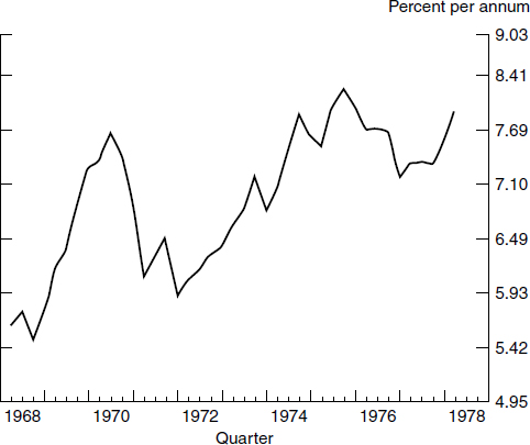
Figure 3.2
Interest rates during the 1970s: Ten-year government bond rate
Most of the concern about economic “paradoxes” in the 1970s was focused on 1974, when a sharp, structural, money-markets shift was believed to have appeared, but could not be explained by interest rate movements. Figure 3.3 displays a source of that concern. Figure 3.3 plots velocity against a bond rate, rather than against time. In figure 3.3 a dramatic shift downward in velocity appears to have occurred in 1974, and clearly that shift cannot be explained by interest rates, since the shift happened suddenly, at a time when little change in interest rates was evident. But observe that this result was acquired using simple sum M3. Figure 3.4 displays the same cross plot of velocity against an interest rate, but with M3 computed as its Divisia index.2 Observe that velocity no longer is constant, either before or after 1974. But no structural shift appears, since the variations in velocity correlate with interest rates. The plot not only has no discontinuous jump at a particular interest rate, but is nearly along a straight (linear) line. Also note that the line slopes in the correct direction: velocity goes up, when interest rates go up.
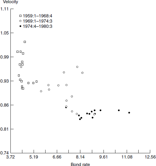
Figure 3.3
Simple sum M3 velocity versus interest rate: Moody’s AAA corporate bond rate, quarterly, 1959:1 to 1980:3
Analogous concerns arose about the supply side of money markets. The reason is evident from figure 3.5, which plots the base multiplier against a bond rate’s deviation from trend.3 The base multiplier is the ratio of a monetary aggregate to the monetary base. Good reason exists for looking at that ratio. The Federal Reserve’s open market operations (purchases and sales of Treasury Bills at the New York Federal Reserve Bank) change the Fed’s balance sheet. Those changes, in turn, change the “monetary base,” which also is called “high powered money,” or outside money. The monetary base is the sum of currency plus bank reserves. Changes in the base work themselves through the banking system and result in a change in the money supply. That is the normal “transmission mechanism” for monetary policy to the money supply, and thereby to inflation and the economy. The ratio of the money supply to the monetary base should exceed 1.0, since bank reserves back a larger amount of bank deposits, with only a fraction of the total deposits being held as reserves. The controllability of the money supply depends heavily on the ability to anticipate the ratio of the money supply to the monetary base. That ratio, also called the base “multiplier,” need not be constant to ensure controllability of the money supply but should be stably related to interest rates, so that the multiplier can be anticipated from current interest rates. Then open market operations can be used to influence the money supply through changes in the monetary base, which is directly under the control of the Federal Reserve through its open market operations.
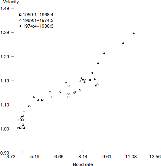
Figure 3.4
Divisia M3 velocity versus interest rate: Moody’s AAA corporate bond rate, quarterly, 1959:1 to 1980:3
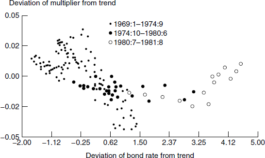
Figure 3.5
Simple-sum M3 base multiplier versus interest rate: deviation from time trend of Moody’s BAA corporate bond rate, monthly, 1969:1 to 1981:8
In figure 3.5 the monetary aggregate is again the simple-sum M3, as computed and officially provided by the Federal Reserve at that time. The base multiplier (adjusted for trend) is plotted against an interest rate. Observe the dramatic structural shift, which is not explained by interest rates. After 1974, the data are along a curved line, in fact a parabola. Prior to 1974, the data are along an intersecting, negatively sloped straight line. This figure displays what appears to be a shocking structural shift. To use the monetary base to control a monetary aggregate before 1974, it would appear to have been necessary to use the straight line to find the multiplier at the observed level of interest rates. After 1974, it would have been necessary to use a completely different intersecting parabola to determine the multiplier at the observed level of interest rates. How could such a thing happen? Perhaps something supernatural happened? But again this puzzle was produced by the simple-sum monetary aggregate. In figure 3.6 the same plot is provided, but with the monetary aggregate changed to Divisia M2. The structural shift is gone.
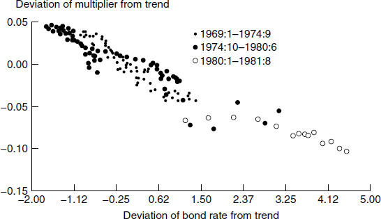
Figure 3.6
Divisia M3 monetary aggregate base multiplier versus deviation from time trend of Moody’s BAA corporate bond interest rate, monthly, 1969:1 to 1981:8
During the late 1970s much was made of the presumed instability of the demand and supply for money. Hundreds of papers were published on the subject, and more significantly these paradoxes were used as a means of trying to discredit the monetarists, who were arguing that the Fed should be held accountable by the Congress for the rate of money creation. The presumed instability of the demand and supply for money was used by the Federal Reserve and some other central banks throughout the world to argue that central banks cannot be held accountable for something that cannot be understood, controlled, or predicted, because of structural shifts and inconsistencies with theory.
A more formal way existed to model the demand for money. The formal method at the time was based on the use of the Goldfeld demand for money equation, which was the standard specification used throughout the Federal Reserve System. The equation was originated by Stephen Goldfeld (1973) at Princeton University. That linear equation sought to explain a monetary aggregate as a function of national income, a regulated interest rate, and an unregulated interest rate.4 As a result three coefficients were on the right-hand side of the equation: the coefficients of each of the three variables. The three coefficients had to be estimated by statistical regression. The equation was widely believed to have become unstable in the 1970s, since the three coefficients seemed to be varying over time. The coefficients were supposed to be constants, with only the variables varying.
P. A. V. B. Swamy and Peter Tinsley (1980), at the FRB in Washington, DC, had produced an approach to estimating a linear equation with the coefficients permitted to vary stochastically over time. The approach permitted testing the hypothesis that the three coefficients were constant with only random noise producing variation around the constants. In that case the appearance of nonconstancy would be statistically insignificant. At the time, Tinsley was my boss at the Federal Reserve Board, and Swamy was a very eminent independent-minded FRB econometrician, who had previously been a full professor at Ohio State University. I asked my boss to arrange for testing of constancy of the Goldfeld equation coefficients, using the Swamy and Tinsley methodology. I requested the test be done twice: once with simple sum M2 on the left-hand side of the equation, as was being done in the Board’s quarterly econometric model, and once with Divisia M2 on the left-hand side. Tinsley passed the job on to Swamy, who had produced the computer program to run the test. He was viewed as being a person of exceptional professional integrity and was not subject to political influence within the system.
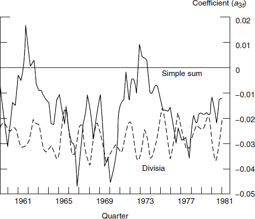
Swamy estimated the model’s three coefficients at the Board with quarterly data from 1959:2 to 1980:4, and the results appeared in Barnett, Offenbacher, and Spindt (1984), which was published in the Journal of Political Economy. The estimated paths of the three coefficients are displayed in figures 3.7, 3.8, and 3.9.5 The solid line is the coefficient path, when money is measured by simple sum M2. The dotted line is the coefficient path, when the monetary aggregate is measured by the Divisia index. The instability of the coefficient is very clear, when the monetary aggregate is simple sum, but the paths look like noise around a constant when the monetary aggregate is Divisia. This conclusion is particularly clear from figures 3.8 and 3.9. Figure 3.8 shows that the coefficient of the unregulated interest rate exhibits clear cycles, when the left-hand side of the equation is simple-sum M2, but little more than noise around a constant, when Divisia M2. In the simple-sum case, the influence of the unregulated interest rate on money is not stable, and the variations in its multiplier are unpredictable.
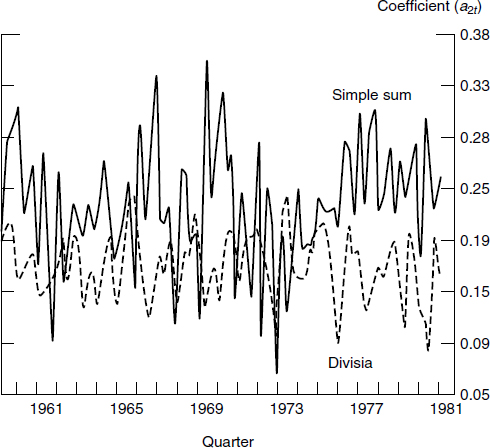
Figure 3.7
Time path of coefficient of income
Figure 3.9 is even clearer. Note that when the left-hand side of the equation is simple-sum M2, the coefficient of the regulated interest rate trends upward for almost half of the two decades, and then trends downward for the rest of the two decades. The influence of the regulated interest rate on money grew for the first part of the period and then declined for the rest of the period, with no measured variable explaining the mysterious trends in that multiplier. In contrast, when the left-hand side of the equation is Divisia money, the coefficient of the regulated interest rate appears to be nothing more than statistically insignificant noise around a constant. In the formal Swamy and Tinsley hypothesis test, stability was rejected jointly for all three coefficients, when the monetary aggregate was simple sum, but not when computed as a Divisia index. In short, when simple-sum M2 was replaced by Divisia M2 on the left side of the Goldfeld equation, the equation worked just fine. No significant evidence existed of instability of the model. No space aliens had landed.
Figure 3.8
Time path of coefficient of market interest rate (commercial paper rate)
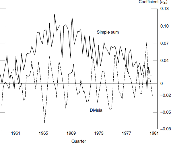
Figure 3.9
Time path of coefficient of regulated interest rate (passbook rate)
Since the Goldfeld equation was the demand for money equation in the Fed’s model at the time, this result was of particular importance to the Board’s model manager, Jerry Enzler. As discussed in section 2.7.3 of chapter 2, Jerry Enzler changed from simple-sum M2 to Divisia M2 in the Board’s quarterly model, used to produce policy simulations. Those simulations provide a menu of “what if” scenarios. In particular, for each proposed policy path for the instruments under the control of the Federal Reserve, the simulation shows what the quarterly model predicts would happen to the economy. These simulations are supplied to the Governors for their use in making policy decisions.
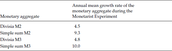
Following the inflationary 1970s, Paul Volcker, as chairman of the Federal Reserve Board, decided to bring inflation under control by decreasing the rate of growth of the money supply, with the instrument of policy being changed from the federal-funds interest rate to nonborrowed reserves.6 The choice of “instrument” of policy is particularly important, since the instrument is the tool the Fed seeks to bring directly under its control, as the means of influencing the inflation rate and general economy. Monetary policy operates through the Fed’s chosen instrument. The period, October 1979 to September 1982, during which the nonborrowed reserves policy applied, was called the “Monetarist Experiment.” The policy succeeded in ending the escalating inflation of the 1970s, but was followed by a recession. That recession, widely viewed as having been particularly deep, was not intended. The existence of widespread three-year negotiated wage contracts was viewed as precluding a sudden decrease in the money growth rate to the intended long-run growth rate. The conclusion, based on a study published by the American Enterprise Institute in Washington, DC, was that such a sudden contraction of monetary growth rate would produce a recession. As a result, the Fed’s decision was to decrease from the high double-digit growth rates to about 10 percent per year and then gradually decrease toward the intended long-run growth rate of about 4 or 5 percent growth rate.
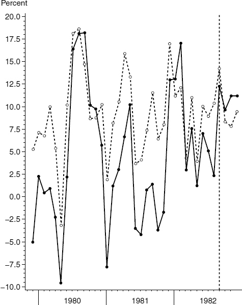
Figure 3.10
Seasonally adjusted annual M2 growth rates. Solid line = Divisia, dashed line = simple sum. The last three observations to the right of the vertical line are post–sample period.
Figures 3.10 and 3.11 and table 3.1 reveal the cause of the unintended recession. As is displayed in figures 3.10 and 3.11, for the M2 and M3 levels of monetary aggregation, the rates of growth of the Divisia monetary aggregates were less than the rates of growth of the official simple-sum aggregates, which were the official targets of policy. As table 3.1 summarizes, the simple-sum aggregates’ growth rates were at the intended levels, but the Divisia growth rates were half as large, producing an unintended negative shock of substantially greater magnitude than intended. A deep recession resulted. That table demonstrates that targeting the official simple-sum monetary aggregates resulted in precisely what was not intended: a rapid drop in the monetary growth rate to 4 or 5 percent per year. When a recession occurred, the unintended consequence was an embarrassment to monetarists, who subsequently denied that a monetarist policy had been in effect. But, as is well known to those who were on the FRB staff at the time, the Fed was doing precisely what it said it was doing, but relative to the simple-sum monetary aggregates.
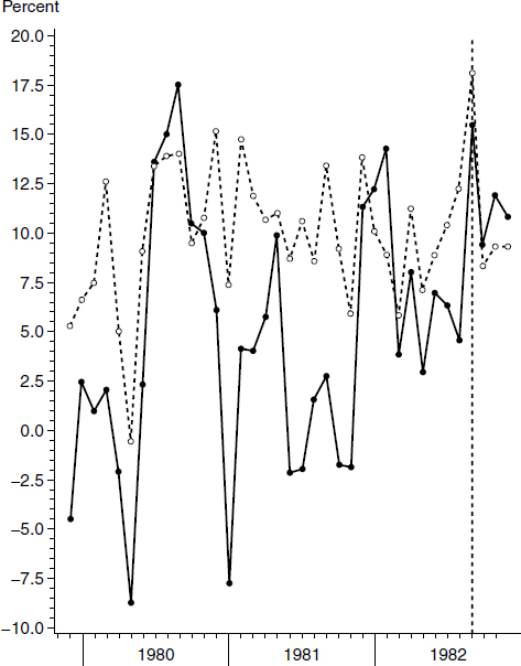
Figure 3.11
Seasonally adjusted annual M3 growth rates. Solid line = Divisia, dashed line = simple sum. The last three observations to the right of the vertical line are post–sample period.
Table 3.1
Mean growth rates during the period
I first published those two figures in the American Statistician, which is a publication of the American Statistical Association. The journal article is Barnett (1984). I am myself a journal editor, of the Cambridge University Press journal, Macroeconomic Dynamics, and have published extensively in professional journals; but submitting this paper was a unique experience. The normal procedure is for the editor to send a submission out to between one and three referees for peer review, before making the decision on whether to publish the article. In this case the editor sent me an astonishingly large number of referee reports, about ten, as I recall. This is virtually unheard of. All of the reports were very favorable, mostly emphasizing the paper’s demonstration of the usefulness of statistics in government policy. In his letter, transmitting to me the unusually large number of very positive reports, the editor said he wanted to talk with me on the telephone. Suffice it to say that no other journal editor has ever asked to talk with me on the phone, and I’ve never asked any author to talk with me on the phone, when I am serving in my role as editor of Macroeconomic Dynamics. Such telephone conversations happen with newspaper article editors, but professional scientific journals simply do not operate that way.
Although surprised by the strange request, I called the editor. He told me the American Statistician has a letters-to-the-editor section, and he was afraid he would be swamped by angry letters to the editor, if he published my article. I responded I was sure my article could alarm some people, but none of them are readers of the American Statistician. He then published the article. No angry letters were sent to the editor.
As I have stated in section 2.7.5 of chapter 2, “Volcker wrote to me years later that he ‘still is suffering from an allergic reaction’ to my findings about the actual monetary growth rate during that period.” The reason for that communication is interesting. With the great Paul Samuelson, I am coauthor of the book, Inside the Economist’s Mind (Barnett and Samuelson 2007). The book contains a collection of the most important interviews I had previously published in the journal, Macroeconomic Dynamics. All the interviews published in that series of interviews are of very eminent economists. The book contains interviews of eight Nobel laureates, two central bank chairmen, and a chairman of the Council of Economic Advisors. One of the economists interviewed is Paul Volcker. With such a distinguished peer group, almost no one I have ever invited to be interviewed has declined, or even hesitated. But Paul Volcker hesitated. For many weeks, he did not respond to my letter of invitation. I wrote again. He then replied he was hesitant because of his “allergic reaction.” He did not go into further detail to explain the reason for his Divisia-monetary-aggregates allergy “problem.” But figures 3.10 and 3.11 and table 3.1 likely go a long way toward explaining his reply. I then assured him I would not personally conduct the interview; he would not be asked anything about my Divisia monetary aggregates; and he could choose the person to conduct the interview. He then accepted, and the interview was completed and published.
That interview is very informative and exceptionally interesting. For example, he makes clear he really did do what he said he was doing during the monetarist experiment, as I knew was true, since I was there. He was using “nonborrowed reserves” as an instrument of policy to bring monetary-aggregate growth rates, and thereby inflation, back down to more reasonable levels.7 The frequently published statement by monetarists, that the Fed was not using nonborrowed reserves to bring down money-supply growth, seemed very strange to the Board’s staff. The staff was being told to do research and provide support for what Volcker said he was doing—and indeed was doing.
The source of that controversy, which continues to the present day, is the fact that targets for the federal-funds interest rate continued to exist during the monetarist experiment period. Some economists were therefore under the impression that no attempt had been made to target nonborrowed reserves, and the policy had remained one of targeting interest rates.8 But arguing it all was a fake amounts to a conspiracy theory, requiring the Federal Reserve Board to have been paying its hundreds of staff economists to work on something not being used at all, while systematically misleading the entire staff to believe otherwise. I do not find that view to be consistent with my experience on the Board staff at that time.9
As Volcker explained, undoubtedly correctly, in Barnett and Samuelson (2007, p. 178):
I used to rankle when some of the members of the Board, who were all enthusiastic about this turn of policy, would say, “Isn’t this just a kind of public relations ploy to avoid being blamed for the rise in interest rates?” I never thought it was that, but a lot of people did think it was largely that. It was a very common thing to say that we just did it to obfuscate. We had no other good benchmark for how much to raise interest rates in the midst of a volatile inflationary situation.
Volcker was one of the Board’s most highly qualified, effective, and brilliant chairmen. Too bad the Board was not using the Divisia monetary aggregates, so the outcome could have been as he had intended.
Following the end of the Monetarist Experiment and the subsequent unintended recession, Milton Friedman became very vocal with his prediction that a huge surge had just appeared in the growth rate of the money supply, and the surge would surely work its way through the economy and produce a new inflation. Since the monetarists, led by Milton Friedman, had been embarrassed in the press by the unexpected recession, resulting from their advocated policy, good reason existed for Friedman to go out on a limb with this prediction, in the hope of recovering the reputation and influence of the monetarist point of view. He went even further by predicting there would be a Federal Reserve overreaction to the inflation, plunging the economy back down into a recession. He published this view repeatedly in the media in various magazines and newspapers, with the most visible being his Newsweek article, which appeared on September 26, 1983. The scanned article is provided in figure 3.12. Some excerpted sentences from that Newsweek article are below:
Figure 3.12
Milton Friedman, Newsweek, September 26, 1983, p. 84
The monetary explosion from July 1982 to July 1983 leaves no satisfactory way out of our present situation. The Fed’s stepping on the brakes will appear to have no immediate effect. Rapid recovery will continue under the impetus of earlier monetary growth. With its historical shortsightedness, the Fed will be tempted to step still harder on the brake—just as the failure of rapid monetary growth in late 1982 to generate immediate recovery led it to keep its collective foot on the accelerator much too long. The result is bound to be renewed stag-flation—recession accompanied by rising inflation and high interest rates. . . . The only real uncertainty is when the recession will begin.
But on exactly the same day, September 26, 1983, I provided a very different view in Forbes magazine. That scanned article is provided in figure 3.13. As with many serious scientists, I rarely talk with the press, but in this case I knew Friedman’s strong views and felt I should go on the record. The following is an excerpt of some of the sentences from that article:
Figure 3.13
William Barnett, Forbes, September 26, 1983, p. 196
People have been panicking unnecessarily about money supply growth this year. The new bank money funds and the super NOW accounts have been sucking in money that was formerly held in other forms, and other types of asset shuffling also have occurred. But the Divisia aggregates are rising at a rate not much different from last year’s . . . the “apparent explosion” can be viewed as a statistical blip.
Of course, Milton Friedman would not have taken such a strong position without reason. You can see the reason from figure 3.14. The percentage growth rates in that figure are monthly, not annualized. When annualized, the large spike in growth rate rises to over 30 percent per year, an enormous inflationary surge—if true. But that solid line is produced from simple sum M2, which was greatly overweighting the newly available, interest-bearing super-NOW accounts and money-market deposit accounts. No spike appeared in the Divisia monetary aggregate, represented by the dashed line, since Divisia removes the nonmonetary, investment motive, which at that time was receiving very high yield.
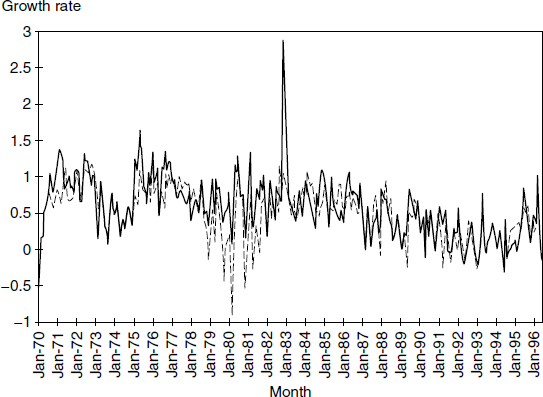
Figure 3.14
Monetary growth rates, 1970 to 1996, from St. Louis Federal Reserve’s database. Solid line is simple-sum money; dashed line is Divisia. As originally published by Barnett (1997), the growth rates are not annualized.
If indeed the huge surge in the money supply growth had really happened, then inflation would surely have followed, unless money is extremely nonneutral (i.e., has no long-run effect on inflation), a view held by very few economists. Friedman undoubtedly was confident that he was right. But no inflationary surge occurred, and no subsequent recession resulted. This comparison of forecasts, published on the exact same day, is one of the few examples in the field of economics of such a documented, controlled-experiment in real time. Friedman’s error resulted from his use of the Fed’s official simple-sum monetary aggregates, which greatly distorted what had happened to the economy’s monetary service flow.
As explained earlier, this chapter in chronological order presents and discusses the history of the “puzzles,” along with the misperceptions those puzzles produced. The current problems in the economy are a consequence. We have now reached the period of 1984 to 1993. But the concerns that arose during that period deal with very technical problems. This section unavoidably surveys a literature that is difficult to explain without a lot of mathematics. If you are not comfortable about the technical jargon in this section, you might want to skim over some of this discussion. You can get the general flavor without biting too deeply into it. The relevant mathematics is presented in appendix D for the benefit of those who would like to acquire a complete understanding of what happened during those years. Some of the more technical details in this subsection are relegated to footnotes. While the rest of the book focuses on the field of economics and its available theory and practice, this section deals with the overlap between economics and finance. As a result much of the technical terminology is from the field of finance.
As described in previous sections, the exact monetary-quantity aggregate can be tracked accurately by the Divisia monetary aggregate, since that tracking ability is known under perfect certainty. But when nominal interest rates are uncertain, the Divisia monetary aggregate’s tracking ability is somewhat compromised. That problem is eliminated by using the extended Divisia monetary aggregate derived by Barnett, Liu, and Jensen (1997) under risk. The extended Divisia monetary-aggregate formula requires risk adjustment, in a manner analogous to the use of “beta” risk adjustments in capital asset pricing in finance. The resulting very complicated formula is derived in appendix D and provided in theorem 1 of that appendix.
Interest rates are not paid in advance. If you were paid interest in advance, you’d take the interest payment up front and immediately withdraw your money from the account or sell the security. The same is true for wages. Workers are paid for their work at the end of the time period during which the work was done. Even with a savings account, you may be quoted an interest rate, when you deposit the funds, but the interest rate may change during the period of your planned holdings. As a rule, short-term interest rates on money-market accounts and securities are subject to low risk. While you cannot be sure of the interest you will receive at the end of the month, the interest payment is not likely to be greatly different from what you expected. So the interest rates in the user-cost price formula, needed to compute the Divisia monetary aggregates, usually can be viewed as low risk. The need for the risk-extended formula is most evident when substantial amounts of foreign denominated money-market and bank-account assets are held. Exchange rate risk can induce high risk into short-term interest rates.
Since Americans do not hold large amounts of such foreign denominated bank accounts, the risk adjustment in the formula is usually not significant.10 But this is not always the case. During the period 1984 to 1993, use grew of money-market funds, stock market funds, and bond funds, all often within packages permitting easy transfer among the account types. The Board’s staff found that once again their official monetary aggregates did not seem to be working properly, and this time the Fed thought the problem had to do with active transfer of funds among money-market funds, stock funds, and bond funds. The Board’s official monetary aggregates included money-market funds but not stock or bond funds. Internalizing that substitution within the monetary aggregates would have required bringing stock and bond funds into the monetary aggregates, although the rates of return on investment in stock and bond funds are subject to substantial risk.
During this time I moved from the University of Texas to Washington University in St. Louis. I produced the extended Divisia aggregate formula with two of my students there, Yi Liu and Mark Jensen, who based much of their doctoral dissertation research on that subject. The result was the extension of the field of index-number theory to the case of risk. François Divisia, along with others who had worked in the field of index-number theory, had based their research on the assumption of perfect certainty about current prices. Our research resulted in a fundamental extension of the literature on index-number theory to the case of uncertain prices and user costs.
With the risk-adjustment extension, Barnett and Xu (1998) demonstrated velocity will change, if the degree of risk of an interest rate changes.11 Hence the variation in the riskiness of an interest rate cannot be ignored in modeling monetary velocity. Applying a small model of the economy, Barnett and Xu (1998) showed the usual computation of velocity will appear to produce instability, when interest rates exhibit varying degrees of risk over time.12 But when the risk-adjusted user-cost variables are used, so that the variation in volatility is not ignored, velocity is stabilized.
Figure 3.15 displays a key role of velocity in the model of the economy, but without risk adjustment. The model was constructed to be stable. Consequently any evidence of instability is misleading. The figure displays a key property of the velocity function: its interest rate slope. We were investigating whether overlooking the risk adjustment could produce erroneous evidence of velocity instability.13 Series 1 was produced with the least variation in interest rate volatility, series 2 with greater variation, and series 3 with even more variable volatility. Note that the plotted velocity property appears to be increasingly unstable, as volatility variation increases. By the model’s construction, the plotted velocity property is constant, if the risk adjustment is used. In addition, with real economic data, Barnett and Xu (1998) showed the evidence of velocity instability in the literature is partially caused by overlooking the variation in the variance of interest rates over time.14
Figure 3.15
Velocity’s simulated interest rate coefficient when there is stochastic volatility of interest rates
Okay, if you have gotten this far, but are confused by the finance terminology, here is the bottom line. During this period of time there was much controversy about the appearance of monetary velocity instability and unpredictability. Here we have the “space alien theory” again, since this instability presumably had no natural economic causes. What my students and I demonstrated was that we could match the patterns of puzzling instability by ignoring the variability of interest rate risk, when in fact it was varying. If we incorporated into the model recognition of the variability of interest rate risk, then the appearance of unexplainable variations of velocity disappeared.
The Divisia index tracks the theoretically exact aggregate, measuring monetary-service flow. But for some purposes the economic capital stock is relevant, especially when investigating wealth effects of policy on the economy. The economic stock of money (ESM), as defined by Barnett (1991), is provided in appendix B in this book’s part II as equation (B.5).15 Comparing the Divisia monetary aggregate flow with the ESM is analogous to comparing the services of a rented apartment during a month, with the services of a purchased condominium during its useful lifetime. Clearly, the rent to use the apartment for one month will be less than the price to buy the condominium. The monetary velocity issue described above was about the service flow, analogous to renting an apartment; but in the rest of this section, the issue is about the capital stock, analogous to buying the apartment as a condominium and using it for multiple years. The relevant theory for measuring the economic capital stock of money is the subject of appendix B. As in the finance field’s capital-asset-pricing theory, the value of the capital stock is the discounted present value of the service flow produced by the stock.
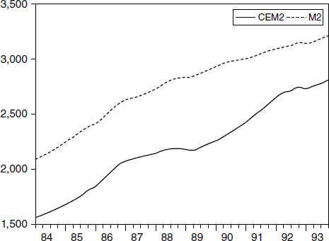
During the late 1980s and early 1990s concern grew about substitution among monetary assets and stock and bond mutual funds, which are not within the monetary aggregates. The FRB staff considered the possibility of incorporating stock and bond mutual funds into the monetary aggregates.16 Barnett and Zhou (1994a) used the formulas discussed above to investigate the problem. The figures supplied in figures 3.16 through 3.19 are from that paper. The dotted line is the simple-sum monetary aggregate, which Barnett (1991) proved is equal to the sum of the economic capital stock of money and the discounted, expected, investment return from the components.17 The simple-sum monetary aggregate measures a joint product, the sum of the discounted investment yield and the discounted monetary-service flow. That proof is provided in appendix B as equation (B.17).
The economic capital stock of money is the monetary stock relevant to macroeconomic theory. Hence we should concentrate on the solid lines in those figures. Note that figure 3.17 displays nearly parallel paths, so the growth rate is about the same for the simple-sum aggregate or the economic stock of money. That figure is for M2+, which was the FRB staff’s proposed, extended aggregate, adding stock and bond mutual funds to M2. But note in figure 3.16 that the gap between the two graphs is decreasing, producing a slower rate of growth for the simple-sum aggregate than for the economic stock of money.
Figure 3.16
M2 joint product and economic capital stock of money. M2 = simple-sum joint product; CEM2 = economic capital stock part of the joint product. Billions of dollars plotted against year.
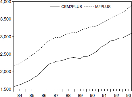
Figure 3.17
M2+ joint product and economic capital stock of money. M2+ = simple-sum joint product; CEM2+ = economic capital stock part of the joint product. Billions of dollars plotted against year.
Figure 3.18
Common-stock mutual-funds joint product and their economic capital stock. StockQ = simple-sum joint product; CEstock = economic capital stock part of the joint product. Billions of dollars plotted against year.
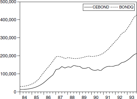
Figure 3.19
Bond mutual funds joint product and their economic capital stock. BondQ = simple-sum joint product; CEbond = economic capital stock part of the joint product. Billions of dollars plotted against year.
The reason can be found in figures 3.18 and 3.19, which use a solid line to display the monetary (i.e., liquidity) services from stock and bond mutual funds. The figures use a dotted line for the simple-sum valuation of those funds, where again the simple sum measures a joint product: the discounted investment yield plus the discounted service flow. Hence the gap between the two lines is the amount motivated by investment yield. Clearly, those gaps had been growing. But it is precisely that gap which does not measure monetary services. By adding the value of stock and bond mutual funds into figure 3.16 to get figure 3.17, the growth rate error of the simple-sum aggregate is offset by adding in more assets providing nonmonetary services. Rather than trying to stabilize the error gap by adding in more and more nonmonetary services, the correct solution would have been to remove the entire error gap by using the solid line in figure 3.16 (or figure 3.17). The solid line measures the actual capital stock of money.
I was invited to present these results at a conference at the Federal Reserve Bank of St. Louis. I asked the audience the following question: Would you consider a Ferrari sports car to be a means of transportation or a source of recreation? Clearly, the price of a Ferrari is too high, if valued solely for its transportation services, and the Ferrari cannot be solely for recreation, since Ferraris are seen on public highways. Ferraris must be a joint product providing both kinds of services. The same has been true of money, since many monetary assets began yielding interest long ago. Two motives exist for holding money: monetary services, such as liquidity, and investment return, such as interest. Investment return is not a monetary service. Otherwise, money would have to include the entire capital stock of the country.
The FRB’s staff had observed something was going wrong with its official simple-sum monetary aggregates. Since nothing was going wrong with the Divisia monetary aggregates, we can see clearly what the source of the problem was. The error gap between the Divisia capital stock and the simple-sum monetary aggregate was narrowing, so the growth rates of the two aggregates were diverging. The error gap is caused by the monetary investment motive, which was declining as people increasingly moved funds out of money and into stock and bond mutual funds. The proposed response by the Board’s staff was to stabilize the gap by bringing in stock and bond mutual funds.
A long history exists of this sort of mistaken approach, by which more and more sources of error were brought into the monetary aggregates in an attempt to stabilize the error component. The right solution is to remove the error gap. Reputable index number theory does exactly that, as with the Divisia monetary aggregates or their discounted, economic capital stock.
The next major concern about monetary aggregates and monetary policy arose at the end of 1999. The financial press became highly critical of the Fed for what was perceived to be a large, inflationary surge in the monetary base. Recall that the monetary base is the sum of currency in the economy and bank reserves. Changes in the monetary base can be viewed as the output produced by the Fed’s open market operations and hence is a primary measure of monetary policy actions. While this interpretation is true, the monetary base is nevertheless a highly defective measure of the effect of monetary policy on the economy, since the base adds together two measures having very different effects on the economy. Currency is dollar-for-dollar pure money. But only a fraction of bank deposit accounts is held as bank reserves. Hence checking accounts are a multiple of bank reserves; and bank account deposits, such as checking accounts, provide monetary services. Variations of bank reserves have a much more powerful “multiplier” effect on the economy than variations of currency, which reflect little more than the need for cash in retail businesses.
Changes in the monetary base are excellent measures of changes in the Fed’s balance sheet and thereby of the Fed’s open market operations. But the defects of the monetary base, as a measure of the consequences of policy for the economy, are well illustrated by the Great Depression of the 1930s. During that period the monetary base steadily grew, as might appear to reflect excellent policy. But the money supply crashed, since bank failures caused the destruction of bank deposits as a multiplier of the decline in the banks’ reserves. Clearly, the crash in money supply was a far more accurate measure of the effects of monetary policy than the steady rise in the monetary base during the Depression.
Near the end of 1999, the reason for the alarming press commentaries is clear from figure 3.20.18 But the reason was not valid, since the cause was again a problem with the data. The so-called Y2K computer bug was expected to cause temporary problems with computers throughout the world, including at banks. Consequently many depositors, including me, withdrew funds from their checking accounts and moved them into cash. While the decrease in deposits thereby produced an equal increase in currency demand, the decrease in deposits produced a smaller decline in reserves because of the multiplier from reserves to deposits. The result was a surge in the monetary base, even though the cause was a harmless, temporary dollar-for-dollar transfer of funds from demand deposits into cash. In addition many bankers feared the computer bug and increased their vault cash as a precaution, with the encouragement of the Federal Reserve. In one such case a banker drove to the St. Louis Fed and filled the trunk of his Cadillac with currency, fearing he would not have enough. A few days later, he returned the cash. Those transfers of funds had little effect on economic liquidity. Once the computer bug was resolved, people put their withdrawn cash back into deposits, and banks returned their excess cash to the Fed, as is seen from figure 3.21.
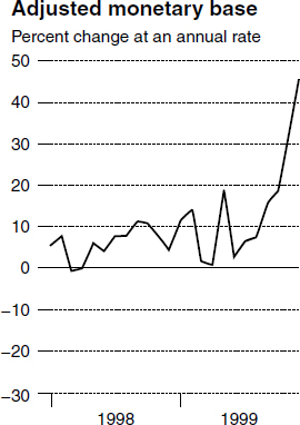
Figure 3.20
Monetary base surge.
The Federal Reserve seemed to recognize the fallacy in the alarmist articles in the press. At the time, I called some of my friends at the Fed and explained that the change in the monetary base was not a reflection of Fed actions on the supply side, but instead was produced by the demand-side actions of depositors worried about the Y2K bug scare. I recommended the Fed ignore the press criticism and not clamp down on the money supply, since the surge in the monetary base would not translate into increased money supply and hence would not produce inflation. The Fed economists I called all agreed with me and said the Fed already understood. Clearly the Fed was right, but again the public (or at least the press) had become confused by the Federal Reserve data.
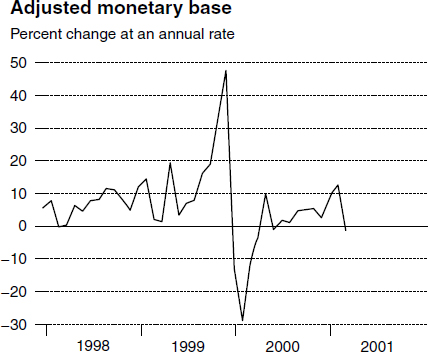
Figure 3.21
Y2K computer bug.
Once upon a time long ago, when monetary assets in the monetary aggregates were limited to cash plus checking accounts, yielding no interest and accepted as means of payment, simple-sum monetary aggregation was consistent with the principles of economic measurement. The Divisia quantity index correctly becomes the simple sum, when the prices of all goods within the aggregate are always equal to each other, since the goods then must be one-for-one perfect substitutes. In the case of monetary aggregation, equal prices mean equal user-cost prices, which can occur only if the interest rates paid on all component assets are equal to each other. Since the rate of interest paid on currency is zero, monetary aggregates validly can be simple sums, only if no interest is paid on any assets within the aggregate.
But those days are long gone, and many monetary assets included in central bank monetary aggregates pay interest. Simple-sum monetary aggregation severely overweights the monetary services of interest-bearing monetary assets, such as certificates of deposit (CDs). By failing to convert to reputable monetary aggregation procedures, the Federal Reserve Board has contaminated the economics literature, misled the public, produced fundamental misperceptions about the abilities of the central bank, and taken away from itself a valuable tool that would have permitted it to make better policy decisions. As financial markets have become more sophisticated, and more and more interest-bearing money market instruments have evolved, the problem has become progressively worse.
1. To facilitate comparison of the plots in figure 3.1, all velocity series were normalized to equal 1.0 in the first quarter of 1968. It should be observed that all index numbers produced from index number theory must be normalized, since only growth rates of statistical index numbers are identified. Levels are determined by cumulating growth rates from the base period, during which the level of the index is set.
2. In figure 3.4 velocity is normalized to equal 1.0 in the first period. As in figure 3.1, normalization is necessary, since only growth rates of statistical index numbers are identified.
3. On the demand side, the plots are against the AAA bond rate. On the supply side, the plots are against the BAA bond rate. These choices were based on the views and experience of my colleagues at the Federal Reserve Board at that time. It was a long time ago, and I do not recall the background that produced that preference. I did it the way that the Fed wanted. I was told to suggest changing one thing at a time, or they would not listen. My preference would have been to plot against the user-cost price, but changing both the quantity aggregation method and the opportunity cost price would have been two things at once.
4. Briefly, that demand for money equation is
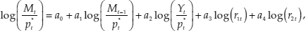
where Mt is the monetary aggregate, ptis the cost of living, measured by the Commerce Department’s index, Yt is GNP (gross national product), r1t is a market interest rate, and r2t is a regulated interest rate. The estimated coefficients are a0, a1, a2, a3, and a4, which normally are treated as constants, but which we permit to vary stochastically over time. Figure 3.7 plots the realization of the stochastic process for a2, figure 3.8 plots the realization of the stochastic process for a3, and figure 3.9 plots the realization of the stochastic process for a4. See equation 6 in Barnett, Offenbacher, and Spindt (1984) for the formal specification of the Goldfeld model’s demand equation.
5. Formally speaking, they are the realizations of the coefficient stochastic processes. Other research in this area includes Serletis (1991).
6. The federal-funds rate is the interest rate that banks charge to each other, when banks borrow from other banks. Nonborrowed reserves are those bank reserves held by banks but not borrowed from the Federal Reserve. A more formal definition and discussion of nonborrowed reserves is provided in section 4.2 of chapter 4.
7. The concept of “nonborrowed reserves” is defined and discussed in section 4.2 of chapter 4.
8. For a serious presentation of that case, see Gilbert (1994).
9. Formally speaking, a possible interpretation of the ambivalent-appearing policy would be that the Federal Reserve was using the federal-funds rate as its instrument and nonborrowed reserves as its intermediate target, where “instruments” of policy are defined to be more closely controllable than “intermediate targets.” Examples of “final targets,” which are the most difficult to control and the most distant in the transmission mechanism of policy, are inflation, unemployment, and economic growth.
10. This conclusion of small risk adjustment with US data is based on the use of the CCAPM (consumption capital asset-pricing model) adjustment in appendix D’s theorem 1. But it is well known in finance that CCAPM, assuming intertemporal separability, underestimates the risk adjustment. Barnett and Wu’s (2005) extension to intertemporal nonseparability, provided in section D.7 of appendix D, has not yet been used to adjust the Divisia monetary aggregates. If the Federal Reserve begins again to provide the consolidated, seasonally adjusted component data on broad monetary aggregates, such as M3—as the Fed should do—then the magnitude of the risk adjustment should be reconsidered with the extended formula in section D.7 of appendix D.
11. We measure risk by the conditional variance of the interest rate stochastic process and permit stochastic volatility.
12. The model was a dynamic stochastic general equilibrium model, which we calibrated.
13. The plotted property is the simulated slope coefficient for the velocity function, treated as a function of the exact interest rate aggregate, but without risk adjustment. All functions in the model are stable, by construction.
14. Subsequently, Barnett and Wu (2005) found that the explanatory power of the risk adjustment increases, if the assumption of intertemporal separability of the utility function is weakened. The separability assumption also is a source of the well-known equity premium puzzle, by which CCAPM under-corrects for risk. Barnett and Wu’s (2005) extension to intertemporal nonseparability is provided in section D.7 of this book’s appendix D.
15. The extension of that economic capital stock formula to risk is available as equation (B.10) in appendix B in this book’s part II, and has been implemented empirically by Barnett, Chae, and Keating (2006).
16. See Collins and Edwards (1994) and Orphanides, Reid, and Small (1994).
17. Computation of the capital stock of money requires modeling expectations. In that early paper, Barnett and Zhou (1994a) used martingale expectations, rather than the more recent approach of Barnett, Chae, and Keating (2006) using VAR forecasting. When martingale expectations are used, the index is called CE.
18. The data is from the St. Louis Federal Reserve Bank’s “adjusted” monetary base. According to its website, the St. Louis Fed “adjusts the monetary base for changes in the demand for base money due to changes in statutory reserve requirement ratios within a given structure of reserve requirements (where the structure defines the types of deposits that are reservable, perhaps by class or type of depository institution), conditional on an assumed model of depository institutions’ demand for base money.”