1

Probability

“Probability is too important to be left to the experts.”

1.1    Introduction

Who has not watched the toss of a coin, the roll of dice, or the draw of a card from a well shuffled deck? In each case, although the initial conditions appear to be much the same, the specific outcome is not knowable. These situations, and many equivalent ones, occur constantly in our society, and we need a theory to enable us to deal with them on a rational, effective basis. This theory is known as probability theory and is very widely applied in our society—in science, in engineering, and in government, as well as in sociology, medicine, politics, ecology, and economics.

How can there be laws of probability? Is it not a contradiction? Laws imply regularity, while probable events imply irregularity. We shall see that many times amid apparent irregularity some regularity can be found, and furthermore this limited regularity often has significant consequences.

How is it that from initial ignorance we can later deduce knowledge? How can it be that although we state that we know nothing about a single toss of a coin yet we make definite statements about the result of many tosses, results that are often closely realized in practice?

Probability theory provides a way, indeed a style, of thinking about such problems and situations. The classical theory has proved to be very useful even in domains that are far removed from gambling (which is where it arose and is still, probably, the best initial approach). This style of thinking is an art and is not easy to master; both the historical evidence based on its late development, and the experience of current teaching, show that much careful thinking on the student’s part is necessary before probability becomes a mental habit. The sophisticated approach of beginning with abstract postulates is favored by mathematicians who are interested in covering as rapidly as possible the material and techniques that have been developed in the past. This is not an effective way of teaching the understanding and the use of probability in new situations, though it clearly accelerates the formal manipulation of the symbols (see the quotation at the top of the Preface). We adopt the slow, cautious approach of carefully introducing the assumptions of the models, and then examining them, together with some of their consequences, before plunging into the formal development of the corresponding theory. We also show the relationship between the various models of probability that are of use in practice; there is not a single model of probability, but many and of differing reliabilities.

Mathematics is not just a collection of results, often called theorems; it is a style of thinking. Computing is also basically a style of thinking. Similarly, probability is a style of thinking. And each field is different from the others. For example, I doubt that mathematics can be reduced to button pushing on a computer and still retain its style of thinking. Similarly, I doubt that the theory of probability can be reduced to either mathematics or computing, though there are people who claim to have done so.

In normal life we use the word “probable” in many different ways. We speak of the probability of a head turning up on the toss of a coin, the probability that the next item coming down a production line will be faulty, the probability that it will rain tomorrow, the probability that someone is telling a lie, the probability of dying from some specific disease, and even the probability that some theory, say evolution, special relativity, or the “big bang,” is correct.

In science (and engineering) we also use probability in many ways. In its early days science assumed there was an exact measurement of something, but there was also some small amount of “noise” which contaminated the signal and prevented us from getting the exact measurement. The noise was modeled by probability. We now have theories, such as information theory and coding theory, which assume from the beginning that there is an irreducible noise in the system. These theories are designed to take account of the noise rather than to initially avoid it and then later, at the last moment, graft on noise. And there are some theories, such as the Copenhagen interpretation of quantum mechanics, which say that probability lies at the foundations of physics, that it is basic to the very nature of the world.

Thus there are many different kinds of probability, and any attempt to give only one model of probability will not meet today’s needs, let alone tomorrow’s. Some probability theories are “subjective” and have a large degree of “personal probability” (belief) as an essential part. Some theories try to be more scientific (objective), and that is the path we will mainly follow—without prejudice to the personal (more subjective) probability approaches which we cannot escape using in our private lives. [Kr, both volumes].

The belief that there is not a single model of probability is rarely held, but it is not unique to the author. The following paraphrase shows an alternate opinion (ignore the jargon for the moment) [G, p.xi,xii]:

In quantum probability theory the state of the system is determined by a complex-valued function A (called the amplitude function) on the outcome space (or sample space). The outcomes of an event E = {x₁, x₂, …} have the probability P(E) of E which is computed by

$P(E)=\hspace{0.17em}|{\displaystyle \sum [A(x_i)]{|}^2}$

This allows for interference as happens in optics and sound. If the outcomes do not interfere, then of course

$P(E)={\displaystyle \sum [|A(x_i)|]}$

This last is the classical probability theory. In the interference case P(E) decomposes into the sum of two parts. The real part is the classical counterpart and the imaginary part leads to the constructive or destructive interference which is characteristic of quantum mechanics and much of physics.

The basic axiom of the path integral formalism is that the state of a quantum mechanical system is determined by the amplitude function A and that the probability of a set of interfering outcomes {x₁, x₂,…} is the first equation. This point has been missed by the axiomatic approaches and in this sense they have missed the essence of quantum mechanics. In principle this essence can be regained by adjoining an amplitude function axiom to the other axioms of the system, but then the axiomatic system is stronger than necessary and may well exclude important cases.

Since we are going to use a scientific approach to probability it is necessary to say what science is and is not. In the past science has tried to be objective and to insist on the property that different people doing the same experiment would get essentially the same results. But we must not assume that science is completely objective, that this repeatability property is perfectly attained or is even essential (for example, consider carefully observational astronomy). Again, if I were to ask two different people to measure the width of a table, one of them might by mistake measure the length, and hence the measurements might be quite different. There is an unstated amount of “understanding what is meant” that is implied in every experimental description. We can only hope to control this assumed background (that is supposed to produce absolute consistency) so that there is little room for error, but we do not believe that we can ever completely eliminate some personal judgment in science. In science we try to identify clearly where judgment comes in and to control the amount of it as best we can.

The statement at the head of this chapter,

Probability is too important to be left to the experts,

is a particular case of a very general observation that the experts, by their very expert training and practice, often miss the obvious and distort reality seriously. The classical statement of this general principle is, “War is too important to be left to the generals.” We daily see doctors who treat cases but not patients, mathematicians who give us exact solutions to the wrong problems, and statisticians who give us verifiably wrong predictions. In our Anglo-Saxon legal system we have clearly adopted the principle that in guilt vs. innocence “twelve tried and true men” are preferable to an experienced judge. The author clearly believes that the same is true in the use of probability; the desire of the experts to publish and gain credit in the eyes of their peers has distorted the development of probability theory from the needs of the average user.

The comparatively late rise of the theory of probability shows how hard it is to grasp, and the many paradoxes show clearly that we, as humans, lack a well grounded intuition in this matter. Neither the intuition of the man in the street, nor the sophisticated results of the experts provides a safe basis for important actions in the world we live in. The failure to produce a probability theory that fits the real world as it is, more or less, can be very costly to our society which uses it constantly.

In the past science has developed mainly from attempts to “measure how much,” to be more precise than general statements such as larger, heavier, faster, more likely, etc. Probability tries to measure more precisely than “more likely” or “less likely.” In order to use the scientific approach we will start (Section 1.5) with the measurement of probability in an objective way. But first some detours and formalities are needed.

1.2    Models in General

It is reasonably evident to most people that all thought occurs internally, and it is widely believed that thinking occurs in the head. We receive stimuli from the external world, (although some sophists have been known to deny the existence of the external world, we shall adopt a form of the “naive realism” position that the world exists and is to some extent “knowable”). We organize our incoming stimuli according to some ill-defined model of reality that we have in our heads. As a result we do not actually think about the real external world but rather we “think” in terms of our impressions of the stimuli. Thus all thought is, in some sense, modeling.

A model can not be proved to be correct; at best it can only be found to be reasonably consistant and not to contradict some of our beliefs of what reality is. Karl Popper has popularized the idea (which goes back at least to Francis Bacon) that for a theory to be scientific it must be potentially falsifiable, but in practice we do not always obey his criterion, plausible as it may sound at first. From Popper’s point of view a scientific theory can only be disproved, but never proved. Supporting evidence, through the application of finite induction, can increase our faith in a theory but can never prove its absolute truth.

In actual practice many other aspects of a model are involved. Occam’s razor, which requires that minimal assumptions be used and extra ones removed, is often invoked as a criterion—we do not want redundant, possibly contradictory assumptions. Yet Occam’s razor is not an absolute, final guide. Another criterion is aesthetic taste, and that depends, among other things, on the particular age and culture you happen to live in. We feel that some theories are nicer than others, that some are beautiful and some are ugly, and we tend to choose the loveliest one in practice. Another very important criterion is “fruitfulness”—does the model suggest many new things to try?

A model is often judged by how well it “explains” some observations. There need not be a unique model for a particular situation, nor need a model cover every possible special case. A model is not reality, it merely helps to explain some of our impressions of reality. For example, for many purposes we assume that a table is “solid,” yet in physics we often assume that it is made of molecules and is mainly “empty space.” Different models may thus seem to contradict each other, yet we may use both in their appropriate places.

In view of the wide variety of applications of probability, past, present, and future, we will develop a sequence of models of probability, generally progressing from the simpler to the more complex as we assume more and more about the model. At each stage we will give a careful discussion of the assumptions, and illustrate some features of them by giving consequences you are not likely to have thought were included in the model. Thus we will regularly discuss examples (paradoxes) whose purpose is to show that you can get rather peculiar results from a model if you are not careful, even though the assumptions (postulates) on the surface seem to be quite bland, [St]. It is irresponsible to teach a probability course as if the contents were entirely safe to use in any situation. As Abelard (1079–1142) said,

“I expose these contradictions so that they may excite the susceptible minds of my readers to the search for truth, and that these contradictions may render their minds more penetrating as the effect of that search.”

Since the applications of probability theory are constantly expanding in range and depth, it is unlikely that anyone can supply models for all the situations that will arise in the future. Hence we are reduced to presenting a series of models, and to discussing some of their relationships, in the hopes that you will be able to create the model you need when the time comes to develop a new one. Each application you make requires you to decide which probability model to adopt.

1.3    The Frequency Approach Rejected

Most people have at least two different models of probability in their minds. One model is that there is a probability to be associated with a single event, the other is that probability is the ratio of the number of successes to the total number of trials in a potentially infinite sequence of similar trials. We need to assume one of these and deduce, in so far as we can, the other from the first—otherwise we risk assuming a contradiction! It will turn out that the two models are not completely equivalent.

A third kind of probability that most people are familiar with is that which arises in betting between friends on sporting events. The “odds” are simply a version of probability; the odds of a to b are the probabilities of a/(a + b) and b/(a + b). There is often no serious thought of repetitions of the event, or a “random selection from an ensemble of similar events,” rather it is the feeling that your “hunches” or “insights” are better than those of the opponent. Both sides recognize the subjective aspect, that two people with apparently the same information can have different probability assignments for the same event. The argument that they have different amounts of information is unconvincing; it is often merely a temporary mood that produces the difference.

The frequency approach (the ratio of the number of successes to the total number of equally likely possible outcomes) seems to be favored by most statistically inclined people, but it has severe scientific difficulties. The main difficulty with the frequency approach is that no one can say how many (necessarily finite) number of trials to make, and it is not practical science to define the probability as the limit of the ratio as the number of trials approaches infinity. Furthermore, the statement of the limiting frequency, in a careful form, will often include the words that you will for any long, finite sequence be only probably close! It is circular to say the least! And you can’t know whether you are looking at an exceptional case or a likely case. It is also true that to get even reasonable accuracy usually requires a discouragingly large number of trials. Finally, there are models, as we shall show in Section 8.7 for which the single event probability has meaning and at the same time the average of n samples has more variability than the original distribution!

For a long time there has been in science a strong trend towards accepting in our theories only objectively measureable quantities and of excluding purely conceptual ones that are only props (like the “ether” in classical physics). The extreme of allowing only measureable quantities is perhaps too rigid an attitude (though a whole school of philosophy maintains this position); yet it is a useful criterion in doing science.

Similarly, there are many mathematical theorems in the literature whose hypotheses cannot be known, even in an intuitive sense, to be close let alone be either exactly true or false within the framework of the intended application; hence these theorems are not likely to be very useful in these practical applications of the theory. Such theorems may be interesting and beautiful pure mathematics but are of dubious applicability.

This “practical use” attitude tends to push one towards “constructive mathematics” [B] and away from the conventional mathematics. The increasing use of computers tends to make many people favor “computable” numbers as a basis for the development of probability theory. Without careful attention to the problem for which it is being used it is not a priori obvious which approach to the real number system we should adopt. And there are some people who regard the continuous mathematics as merely a useful approximation to the discrete since usually the equivalent operations are easier in the continuous model than they are in the discrete. Furthermore, quantum mechanics suggests, at least to some people, that ultimately the universe is discrete rather than continuous.

Whenever a new field of application of mathematics arises it is always an open question as to the applicability of the mathematics which was developed earlier; if we are to avoid serious blunders it must be carefully rethought. This point will be raised repeatedly in this book.

For these and other reasons we will not begin with the frequency approach, but rather deduce (Sections 2.8 and Appendix 2.A) the frequency model along with its limitations. For this present Section see [Ke], especially Chapter 8.

1.4    The Single Event Model

In most fields of knowledge it is necessary, sooner or later, to introduce some technical notation and jargon so that what is being talked about is fairly precise and we can get rid of the vagueness of words as used in normal language. We have used some of these words already!

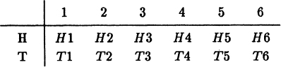
At first a trial is a single unit, like the toss of a coin, the roll of a die (singular of dice), or the draw of a single card from a well shuffled deck. The elementary events of a trial are the possible outcomes of the trial. For example, for the toss of a coin the elementary events are “head” and “tail.” For the roll of a die the elementary events are the names of the six faces, 1,2,3,4,5,6. The elementary events are considered to be indivisible, atomic, events from which more complex events (say an even numbered face of a die) may be built. We will label the possible outcomes of a trial by the symbols x_i, where i runs from 1 to n (or possibly 0 to n). Thus as a first approximation, to be modified later, we have the trial labeled X whose outcome is some particular x_i. The capital letter X represents the trial, and the set {x_i} represents the possible outcomes of the trial; some particular x_i will be the actual outcome of the trial X being conducted. In some circumstances the symbol X may be thought of as being the whole set {x_i} just as the function sin x may be thought of as the entire function. This list of possible outcomes is an idealization of reality. Initially we assume that this list is finite in length.

Later on a trial may be a sequence of these simple trials; the roll of, say, four dice at one time will be a single trial. Still later we will continue for an indefinite number of times until some condition is reached such as tossing a coin until three heads occur in a row. In such cases the entire run will be considered a single trial, and the number of possible events will not be finite but rather countably infinite. Still later, we will examine a continuum of events, a classically non-countable number of events.

In principle the first step in a discrete probability problem is, for the trial (named) X, to get the corresponding list (or set) X of all the possible outcomes x_i. Thus X has two meanings; it is the name of the trial and it is also the list of possible the outcomes of the trial. The name of the outcome should not be logically confused with any value associated with the outcome. Thus logically the face “the number of spots,” say 4, on a die is a label and should not be confused with the name “four,” nor with the value “4” that is usually associated with this outcome. In practice these are often carelessly treated as being the same thing.

The beginner is often confused between the model and reality. When tossing a coin the model will generally not include the result that the coin ends up on its edge, nor that it is lost when it rolls off the table, nor that the experimenter drops dead in the middle of the trial. We could allow for such outcomes if we wished, but they are generally excluded from simple problems.

In a typical mathematical fashion these events (outcomes) x_i are considered to be points in the sample space X; each elementary event x_i is a point in the (at present) finite, discrete sample space. To get a particular realization of a trial X we “sample” the sample space and select “at random” (to be explained in more detail in Section 1.9) an event x_i. The space is also called a list (as was stated above) and we choose (at random) one member (some x_i) of the list X as the outcome of the trial.

1.5    Symmetry as the Measure of Probability

With this notation we now turn to the assignment of a measure (the numerical value) of the probability p_i to be associated with (assigned to) the event x_i of the trial.

Our first tool is symmetry. For the ideal die that we have in our mind we see that (except for the labels) the six possible faces are all the same, that they are equivalent, that they are symmetric, that they are interchangeable. Only one of the elementary events x_i can occur on one (elementary) trial and it will have the probability p_i. If any one of several different outcomes x_i is allowed on a trial (say either a 4 or a 6 on a roll of a die) then we must have the “additivity” of probabilities p_i. For the original sample space we will get the same probability, due to the assumed symmetry, for the occurences of each of the elementary events. We will scale this probability measure so that the sum of all the probabilities over the sample space of the elementary events must add up to 1.

If you do not make equal probability assignments to the interchangeable outcomes then you will be embarrassed by interchanging a pair of the nonequal values. Since the six faces of an ideal die are all symmetric, interchangeable if you prefer, then each face must have the probability of 1/6 (so that the total probability is 1). For a well shuffled ideal deck of cards we believe that each of the 52 cards are interchangeable with every other card so each card must have a probability of 1/52. For a well balanced coin having two symmetric faces each side must have probability 1/2.

Let us stop and examine this crucial step of assigning a measure (number) p_i called “the probability” to each possible outcome x_i of a trial X. These numbers are the probabilities of the elementary events. From the perceived symmetry we deduced interchangeability, hence the equality of the measure of probability of each of the possible events. The reasonableness of this clearly reinforces our belief in this approach to assigning a measure of probability to elementary events in the sample space.

This perception of symmetry is subjective; either you see that it is there or you do not. But at least we have isolated any differences that may arise so that the difference can be debated sensibly. We have proceeded in as objective a fashion as we can in this matter.

However, we should first note that, “Symmetric problems always have symmetric solutions.” is false [W]. Second, when we say symmetric, equivalent, or interchangable, is it based on perfect knowledge of all the relevant facts, or is it merely saying that we are not aware of any lack thereof? The first case being clearly impossible, we must settle for the second; but since the second case is vague as to how much we have considered, this leaves a lot to be desired. We will always have to admit that if we examined things more closely we might find reason to doubt the assumed symmetry.

We now have two general rules: (1) if there are exactly n different inter changeable (symmetric in some sense) elementary events x_i, then each event x_i has probability p_i = 1/n since (2) the probabilities of the elementary events in the sample space are additive with a total probability of 1.

Again, from the additivity of the probabilities of the elementary events it follows that for more complex situations when there is more than one point in the sample space that satisfies the condition then we add the individual probabilities.

For the moment we will use the words “at random” to mean equally likely choices in the sample space; but even a beginner can see that this is circular—what can “equally likely” mean except equally probable, (which is what we are trying to define)? Section 1.9 will discuss the matter more carefully; for the moment the intuitive notion will suffice to do a few simple problems.

Example 1.5–1    Selected Faces of a Die

Suppose we have a well balanced die and ask for the probability that on a random throw the upper face is less than or equal to 4.

The admissible set of events (outcomes) is {x_i} = {1,2,3,4}. Since each has probability p_i = 1/6, we have

$\text{Prob }\{x_i\le 4\}=1/6+1/6+1/6+1/6=4/6=2/3$

If instead we ask for the probability that the face is an even number, then we have the acceptable set {2,4,6}, and hence

$\text{Prob }\left\{x_i\text{ even}\right\}=1/6+1/6+1/6=3/6=1/2$

Example 1.5–2    A Card With the Face 7

What is the probability that on the random draw of a card from the standard card deck of 52 cards (of 4 suits of 13 cards each) that the card drawn has the number 7 on it?

We argue that there are exactly 4 cards with a 7 on their face, one card from each of the four suits, hence since the probability of a single card is 1/52 we must have the probability

$\text{Prob {face}=\text{7}}=4/52=1/13.$

There are other simple arguments that will lead to the same result.

Example 1.5–3    Probability of a Spade

What is the probability of drawing a spade on a random draw from a deck of cards?

We observe that the probability of any card drawn at random is 1/52. Since there are 13 spades in the deck we have the combined probability of

$P(\text{spade})=(13)(1/52)=1/4$

Exercises 1.5

1.5–1. If there are 26 chips each labeled with a different letter of the alphabet what is the probability of choosing the chip labeled Q when a chip is drawn at random? Of drawing a vowel (A, E, I, O, U)? Of not drawing a vowel? Ans. 1/26, 5/26, 21/26.

1.5–2. If 49 chips are labeled 1,2,… 49, what is the probability of drawing the 7 at random? A number greater or equal to 7? Ans. 1/49, 43/49.

1.5–3. If 49 chips are labeled 2,4,… 98, what is the probability of drawing the chip 14 at random? Of a number greater than 20?

1.5–4 A plane lattice of points in the shape of a square of size n > 2 has n² points. What is the probability of picking a corner point? The probability of picking an inner point? Ans. 4/n², [(n − 2)/n]²

1.5–5 A day of the week is chosen at random, what is the probability that it is Tuesday? A “weekday”?

1.5–6 We have n³ items arranged in the form of a lattice in a cube, and we pick at random an item from an edge (not on the bottom). What is the probability that it is a corner item? Ans. 1/(2n − 3).

1.5–7 In a set of 100 chips 10 are red; what is the probability of picking a red chip at random? Ans. 1/10.

1.5–8 If there are r red balls, w white balls, and b blue balls in an urn and a ball is drawn at random, what is the probability that the ball is red? Is white? Is blue? Ans. r/(r + w + b), w/(r + w + b), b/(r + w + b).

1.5–9 There are 38 similar holes in a roulette wheel. What is the probability of the ball falling in any given hole?

1.5–10 In a deck of 52 cards what is the probability of a random drawing being the 1 (ace) of spades? Of drawing at random a heart? Ans. 1/52,1/4

1.5–11 There are 7 bus routes stopping at a given point in the center of town. If you pick a bus at random what is the probability that it will be the one to your house?

1.5–12 In a box of 100 items there are 4 defective ones. If you pick one at random what is the probability that it is defective? Ans. 1/25

1.5–13 If 3% of a population has a certain disease what is the probability that the next person you pass on the street has it? Ans. 0.03

1.5–14 Due to a malajustment a certain machine produces every fifth item defective. What is the probability that an item taken at random is defective?

1.5–15 In a certain class of 47 students there are 7 with last names beginning with the letter S. What is the probability that a random student’s name will begin with the letter S? Ans. 7/47

1.6    Independence

The next idea we need is independence. If we toss a coin and then roll a die we feel that the two outcomes are independent, that the outcome of the coin has no influence on the outcome of the die. The sample space is now

We regard this sample space as the product of the two elemetary sample spaces. This is often called the Cartesian (or direct) product by analogy with cartesian coordinates of the two original sample spaces, {H,T} for the coin, and {1,2,3,4,5,6} for the die. Since we believe that the outcomes of the die and coin are independent we believe (from symmetry) that the events in the product sample space are all equally likely, hence each has probability 1/(2 × 6) = 1/12. We see that the probability of the compound events in the product sample space are (for independent events) just the product of the corresponding probabilities of the separate original events, that

$1/12=(1/2)(1/6).$

Clearly the product space (meaning the product of the sample spaces) of the coin with the die is the same as the product space of the die with the coin.

We immediately generalize to any two independent events, each of these being from an equally likely sample space. If there are n₁ of the first kind of event and of the second, then the product space of the combined trial has n₁n₂ events each of the same probability $1/n_1{n}_2=(1/n_1)(1/n_2)$.

Example 1.6–1    The Sample Space of Two Dice

Consider the toss of two independently rolled dice. The sample space has 6 × 6 = 36 events each of probability 1/36, and the sample space is:

$\begin{array}{ccccc}1,1& 1,2& 1,3& \cdots & 1,6\\ 2,1& 2,2& 2,3& \cdots & 2,6\\ \cdots & \cdots & \cdots & \cdots & \cdots \\ 6,1& 6,2& 6,3& \cdots & 6,6\end{array}$

Clearly the idea of a product space may be extended to more than two independent things.

Example 1.6–2    The Sample Space of Three Coins

Consider the toss of three coins. We have 2 × 2 × 2 = 8 equally likely outcomes. It is awkward to draw 3 dimensional sample spaces, and it is not feasible to draw higher dimensional sample spaces, so we resort to listing the elementary events. For the three coins we have a list (equivalent to the product sample space)

$\begin{array}{cccccccc}HHH& HHT& HTH& THH& HTT& THT& TTH& TTT\end{array}$

each of probability (1/2)(1/2)(1/2) = 1/8.

The extension to m different independent trials each having n_i(i = l,2,…,m) equally likely outcomes leads to a product space of size equal to the product n₁n₂…n_m of the dimensions of the original spaces. The probabilities of the events in the product space are equal to the corresponding products of the probabilities of the original events making up the original spaces, hence the product space events are also equally likely (since the original ones were equally likely).

Example 1.6–3    The Number of Paths

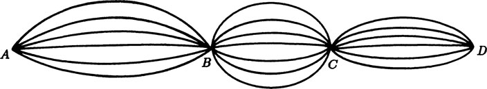
If you can go from A to B in 6 ways, from B to C in 7 ways, and from C to D in 5 ways, then there are 6 × 7 × 5 = 210 ways of going from A to D, Figure 1.6–1. If each of the original ways were equally likely and independent then each of the 210 ways is also equally likely and has a probability of 1/210.

FIGURE 1.6–1

Notice again, the probabilities of the equally likely events in the product sample space can be found by either: (1) computing the number of events x_i in the product space and assigning the same probability p_i = 1/(the number of events) to each event in the product space, or (2) assign the product of the probabilities of the separate parts to each compound event in the product space.

Notice also that we are always assuming that the elementary points in the sample space are independent of each other, that one outcome is not influenced by earlier choices. However, in this universe in which we live apparently all things are interrelated (“intertwined” is the current jargon in quantum mechanics); if so then independence is an idealization of reality, and is not reality.

It is easy to make up simple examples illustrating this kind of probability problem, and working out a large number of them is not likely to teach you as much as carefully reviewing in your mind why they work out as they do.

Exercises 1.6

1.6–1 What is the probability of HHH on the toss of three coins when the order of the outcomes is important? Of HTH? Of TTH? Ans. 1/8.

1.6–2 Describe the product space of the draw of a card and the roll of a die.

1.6–3 What is the size of the product space of the roll of three dice? Ans. 6³ = 216.

1.6–4 What is the size of the product space of the toss of n coins? Ans. 2ⁿ.

1.6–5 What is the size of the product space of the toss of n dice?

1.6–6 What is the product space of a draw from each of two decks of cards? Ans. Size= (52)².

1.6–7 What is the size of the sample space of independent toss of a coin, roll of a die, and the draw of a card?

1.7    Subsets of a Sample Space

We are often interested not in all the individual outcomes in a product space but rather only those outcomes which have some specific property. We have already done a few such cases.

Example 1.7–1    Exactly One Head in Three Tosses

Suppose we ask in how many ways can exactly one head turn up in the toss of three coins, or equivalently, what is the probability of the event. We see that in the complete sample space of 8 possible outcomes we are only interested in the three events

$\begin{array}{ccc}HTT& THT& TTH\end{array}$

Each of these has a probability of 1/8, so that the sum of these will be 3/8 which is the corresponding probability.

Clearly we are using the additivity of the probabilities of the events in the sample space. We need to know the size of the sample space, but we need not list the whole original sample space, we need only count the number of successes. Listing things is merely one way of counting them.

Example 1.7–2    Sum of Two Dice

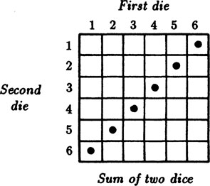
What is the probability that the sum of the faces of two independently thrown dice total 7? We have only the six successful possibilities

$\begin{array}{cccccc}1+6,& 2+5,& 3+4,& 4+3,& 5+2,& 6+1\end{array}$

in the total sample space of 6² = 36 possible outcomes. See Figure 1.7–1. Each possible outcome has probability of 1/36, hence the probability of a total of 7 is 6/36 = 1/6.

FIGURE 1.7–1

We can look at this in another way. Regardless of what turns up on the first die, there is exactly one face of the second that will make the total equal to 7, hence the probability of this unique face is 1/6.

If we were to ask in how many ways, (or equivalently what is the probability), can the sum of three or four, or more dice add up to a given number then we would have a good deal of trouble in constructing the complete sample space and of picking out the cases which are of interest. It is the purpose of the next two chapters to develop some of the mathematical tools to carry out this work; the purpose of the present chapter is to introduce the main ideas of probability theory and not to confuse you by technical details, so we will not now pursue the matter much further.

We now have the simple rule: count the number of different ways the compound event can occur in the original sample space of equally likely events (outcomes), then the probability of this compound event is the ratio of the number of successes in the sample space to the total number of events in the original sample space.

Aside: Probability Scales

We have evidently chosen to measure probability on a scale from 0 to 1, with 0 being impossibility and 1 being certainty. A scale that might occur to you is from 1 to infinity, which is merely the reciprocal of the first range, (you might also consider 0 to infinity). In these cases you will find that the addition of probabilities is not simple. There are other objections that you can find if you choose to explore these scales.

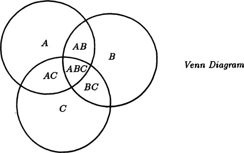
FIGURE 1.7–2

A Venn diagram is mainly a symbolic representation of the subsets of a sample space. Typically circles are used to represent the subsets, see Figure 1.7–2. The subsets represented are the insides of the circles A,B and C. Now consider those events which have both properties A and B, shown by the region AB. Similarly for the sets AC and BC. Finally, consider the events which have the properties of A, B and C at the same time; this is the inner piece in the diagram, ABC. In this simple case the representation is very illuminating. But if you try to go to very many subsets then the problem of drawing a diagram which will show clearly what you are doing is often difficult; circles are not, of course, necessary, but when you are forced to draw very snake-like regions then the diagram is of little help in visualizing the situation. In the Venn diagram the members of a set are often scattered around (in any natural display of the elements of the sample space), hence we will not use Venn diagrams in this book.

Exercises 1.7

1.7–1 What is the probability of a die showing an odd digit?

1.7–2 What is the probability of drawing a “diamond” when drawing a card from a deck of 52 cards? Ans. 1/4.

1.7–3 On the roll of two dice what is the probability of getting at least one face as a 4? Ans. 11/36.

1.7–4 What is the probability of two H’s in two tosses of a coin?

1.7–5 On the roll of two independent dice what is the probability of a total of 6? Ans. 5/36.

1.7–6 Make a Venn diagram for four sets.

1.7–7 In a toss of three coins what are the probabilities of 0,1,2, or 3 heads? Ans. 1/8,3/8,3/8,1/8.

1.7–8 What is the probability of drawing either the 10 of diamonds or the jack of spades?

1.7–9 What is the probability of drawing an “ace” (ace= 1), jack, queen or king from a deck of 52 cards? Ans. 4/13.

1.7–10 What is the probability of drawing a black card from the deck?

1.7–11 If two dice are rolled what is the probability both faces are the same? Ans. 1/6.

1.7–12 If three dice are rolled what is the probability that all three faces are the same? Ans. 1/36.

1.7–13 If a coin is tossed n times what is the probability that all the faces are the same? Ans. 1/2^n–1

1.7–14 If one card is drawn at random from each of two decks of cards what is the probability that the two cards are the same? Ans. 1/52.

1.7–15 Odd man out. Three people each toss a coin. What is the probability of some person being the “odd man out”? Ans. 3/4.

1.7–16 If 4 people play odd man out what is the probability that on a round of tosses one person will be eliminated? Ans. 1/2.

1.7–17 On the toss of two dice what is the probabilty that at least one face has a 4 or else that the sum of the faces is 4? Ans. 1/18.

1.7–18 Same as 1.7–17 except the number is 6 (not 4). Ans. 4/9.

1.8    Conditional Probability

Frequently the probability we want to know is conditional on some event. The effect of the condition is to remove some of the events in the sample space (list), or equivalently to confine the admissable items of the sample space to a limited region.

Example 1.8–1    At Least Two Heads in Ten Tosses

What is the probability of at least two heads in the toss of 10 coins, given that we know that there is at least one head.

The initial sample space of 2¹⁰ = 1024 points is uncomfortably large for us to list all the sample points, even when some are excluded; and we do not care to list even the successes. Instead of counting we will calculate the number of successes and the size of the entire sample space.

We may compute this probability in two different ways. First we may reason that the sample space now excludes the case of all tails, which can occur in only one way in the sample space of 2¹⁰ points; there are now only 2¹⁰ − 1 equally likely events in the sample space. Of these there are 10 ways in which exactly one head can occur, namely in any one of the ten possible positions, first, second, …, tenth. To count the number of events with two or more heads we remove from the counting (but not from the sample space) these 10 cases of a single head. The probability of at least two heads is therefore the ratio of the number of successes (at least 2 heads) to the total number of events (at least one head)

$(2^{10}-1-10)/(2^{10}-1)=1013/1023=0.9902\dots$

Secondly, we could use a standard method of computing not what is wanted but the opposite. Since this method is so convenient, we need to introduce a suitable notation. If p is the probability of some simple event then we write q = 1 – p as the probability of it not happening, and call it the complement probability. Given the above ten coin problem we can compute the complement event, the probability Q that there was one head, and then subtract this from 1 to get

$P=1-Q=1-10/(2^{10}-1)$

As a matter of convenient notation we will often use lower case letters for the sample space probabilities and upper case letters for the probabilities of the compound events.

Example 1.8–2    An Even Sum on Two Dice

On the roll of two independent dice, if at least one face is known to be an even number, what is the probability of a total of 8?

We reason as follows. One die being even and the sum is to be 8 hence the second die must also be even. Hence the three equally likely successes (the sum is 8) in the sample space are

$\begin{array}{ccc}2,6& 4,4& 6,2\end{array}$

out of a total sample space of {36 – (both faces odd)} = 36 − 3 × 3 = 27. Hence the probability is 3/27 = 1/9.

Example 1.8–3    Probability of Exactly Three Heads Given that there are at Least Two Heads

What is the probability of exactly three heads knowing that there are at least two heads in the toss of 4 coins?

We reason as follows. First, how many cases are removed from the original complete sample space 2⁴ = 16 points? There is the single case of all tails, and the four cases of exactly 1 head, a total of 5 cases are to be excluded from the original 16 equally likely possible cases; this leaves 11 still equally likely events in the sample space. Second, for the three heads there are exactly 4 ways that the corresponding 1 tail can arise, (HHHT, HHTH, HTHH, THHH), so there are exactly 4 successes. The ratio is therefore 4/11 = the probability of exactly three heads given that there are at least two heads.

Exercises 1.8

1.8–1 If a fair coin is tossed 10 times what is the probabilty that the first five are the same side? Ans. 1/16 = 6.25%.

1.8–2 Given that the sum of the two faces of a pair of dice is greater than 10, what is the probability that the sum is 12? Ans. 1/3.

1.8–3 In drawing two cards from a deck (without returning the first card) what is the probability of two aces when you get at least one ace?

1.8–4 What is the probability of different faces turning up on two tosses of a die? Ans. 5/6.

1.8–5 What is the probability of no two faces being the same on three tosses of a die? Ans. 5/9.

1.8–6 What is the probability that at least one face is a 6 on the toss of a pair of dice, given that the sum is ≥ 10? Ans. 5/6.

1.8–7 Given that in four tosses of a coin there are at least two heads, what is the probability that there are at least three heads?

1.8–9 Given that both faces on the toss of two dice are odd, what is the probability of at least one face being a 5? Ans. 5/9.

1.8–10 In n tosses of a coin, given that there are at least two heads, what is the probability of n or n− 1 heads?

1.8–11 Given that two cards are honor cards (10, J,Q, K, A) in spades what is the probability that exactly one of them is the ace? Ans. 8/25.

1.8–12 Given that a randomly drawn card is black, what is the probability that it is an honor card? Ans. 10/26 = 5/13.

1.8–13 Given that an even number of heads show on the toss of 4 coins (0 is an even number), what is the probability of exactly 2 heads? Ans. 3/4.

1.8–14 On the toss of three coins what is the probability of an even number of heads? Ans. 1/2.

1.8–15 On the toss of 4 coins what is the probability of an even number of heads?

1.8–16 From the previous two problems what is the probability of an even number of heads on the toss of n coins? Ans. 1/2.

1.8–19 Given that the sum of the faces on two dice is 6, what is the probability that one face is a 4? Ans. 2/5.

1.8–20 Given that each of the faces on three dice show even number, what is the probability of at least one face being a 6?

1.9    Randomness

Randomness is a negative property; it is the absence of any pattern (we reject the idea that the absence of a pattern is a pattern and for set theory formalists this should be considered carefully). Randomness can never be proved, only the lack of it can be shown. We use the absence of a pattern to assert that the past is of no help in predicting the future, the outcome of the next trial. A random sequence of trials is the realization of the assumption of independence—they are the same thing in different forms. Randomness is “a priori” (before) and not “a posteriori” (after).

We have not defined “pattern.” At present it is the intuitive idea that if there is a pattern then it must have a simple description—at least simpler than listing every element of the pattern.

Randomness is a mathematical concept, not a physical one. Mathematically we think of random numbers as coming from a random source. Any particular sequence of numbers, once known, is then predictable and hence cannot be random. A reviewer of the famous RAND [R] Table of a Million Random Numbers caught himself in mid review with the observation that now that they had been published the numbers were perfectly predictable (if you had the table) and therefore could not be random! Thus the abstract mathematical concept of a random sequence of numbers needs to be significantly modified when we actually try to handle particular realizations of randomness.

In practice, of course, you can have only a finite sequence of numbers, and again, of course, the sequence will have a pattern, if only itself! There is a built in contradiction in the words, “I picked a random number between 1 and 10 and got 7.” Once selected (a posteriori) the 7 is definite and is not random. Thus the mathematical idea of random (which is a priori) does not match closely what we do in practice where we say that we have a random sample since once obtained the random sample is now definite and is not mathematically random. Before the roll of a die the outcome is any of the 6 possible faces; after the roll it is exactly one of them. Similarly, in quantum mechanics before a measurement on a particle there is the set of possible outcomes (states); after the measurement the particle is (usually) in exactly one state.

On most computers we have simple programs that generate a sequence of “pseudo random numbers” although the word “pseudo” is often omitted. If you do not know that they are being generated by a simple formula then you are apt to think that the numbers are from a random source since they will pass many reasonable tests of randomness; each new pseudo random number appears to be unpredictable from the previous ones and there appears to be no pattern (except that for many random number generators they are all odd integers!), but if you know the kind of generating formula being used, and have a few numbers, then all the rest are perfectly predictable. Thus whether or not a particular stream of numbers is to be regarded as coming from a random source or not depends on your state of knowledge—an unsatisfactory state of affairs!

For practical purposes we are forced to accept the awkward concept of “relatively random” meaning that with regard to the proposed use we can see no reason why they will not perform as if they were random (as the theory usually requires). This is highly subjective and is not very palatable to purists, but it is what statisticians regularly appeal to when they take “a random sample” which once chosen is finite and definite, and is then not random—they hope that any results they use will have approximately the same properties as a complete counting of the whole sample space that occurs in their theory.

There has arisen in computing circles the idea that the measure of randomness (or if you wish, nonrandomness) should be via the shortest program that will generate the set of numbers (without having carefully specified the language used to program the machine!). This tends to agree with many people’s intuitive feelings – it should not be easy to describe the lack of a pattern in any simple fashion, it ought to be about as hard as listing all the random numbers. Thus the sequence

$\begin{array}{ccccccccc}0& 1& 0& 1& 0& 1& 0& 1& 0\dots \end{array}$

is “more random” than is the sequence

$\begin{array}{ccccccccc}0& 0& 0& 0& 0& 0& 0& 0& 0\dots \end{array}$

but is less random than the sequence

$\begin{array}{cccccccccccccccc}0& 1& 0& 0& 0& 1& 1& 0& 1& 1& 0& 0& 0& 0& 0& 1\dots \end{array}$

In this approach pseudo random numbers are only slightly random since the program that generates them is usually quite short! It would appear that a genuinely mathematically random number generator cannot be written in any finite number of symbols!

We will use the convenient expression “chosen at random” to mean that the probabilities of the events in the sample space are all the same unless some modifying words are near to the words “at random.” Usually we will compute the probability of the outcome based on the uniform probability model since that is very common in modeling simple situations. However, a uniform distribution does not imply that it comes from a random source; the numbers 1,2,3, …, 6n when divided in this order by 6 and the remainders (0,1,2,3,4,5) tabulated, gives a uniform distribution but the remainders are not random, they are highly regular!

These various ideas of randomness (likeliness) are not all in agreement with our intuitive ideas, nor with each other. From the sample space approach we see that any hand of 13 cards dealt from a deck of 52 cards is as likely as any other hand (as probable—as random). But the description of a hand as being 13 spades is much shorter than that of the typical hand that is dealt. Furthermore, the shortness of the description must depend on the vocabulary available—of which the game of bridge provides many special words. We will stick to the sample space approach. Note that the probability of getting a particular hand is not connected with the “randomness of the hand” so there is no fundamental conflict between the two ideas.

If this idea of a random choice seems confusing then you can take comfort in this observation: while we will often speak of “picking at random” we will always end up averaging over the whole sample space, or a part of it; we do not actually compute with a single “random sample.” This is quite different from what is done in statistics where we usually take a small “sample” from the sample space and hope that the results we compute from the sample are close to the ideal of computing over the complete sample space.

Example 1.9–1    The Two Gold Coins Problem

There is a box with three drawers, one with two gold coins, one with a gold and a silver coin, and one with two silver coins. A drawer is chosen at random and then a coin in the drawer is chosen at random. The observed coin is gold. What is the probability that the other coin is also gold?

The original sample space before the observation is clearly the product space of the three random drawers and the two random choices of which coin, (in order to count carefully we will give the coins marks 1 and 2 when there are two of the same kind, but see Section 2.4)

$\begin{array}{ccc}& \text{Order}& \\ & \text{first/second}& \text{first/second}\\ \text{drawer 1}& G_1{G}_2& G_2{G}_1\\ \text{drawer 2}& GS& SG\\ \text{drawer 3}& S_1{S}_2& S_2{S}_1\end{array}$

These six cases, choice of drawer (p = 1/3), and then choice of which coin (p = 1/2), exhaust the sample space. Thus each compound event has a probability of 1/6. Since, as we observed, high dimensional spaces are hard to draw, we shift to a listing of the elementary events as a standard approach.

$\begin{array}{ccc}\text{first drawer}& \text{second drawer}& \text{third drawer}\\ G_1{G}_2,G_2{G}_1,& GS,S{G}^{*},& S_1{S}_{2*},S_2{S}_{1*}\end{array}$

In this sample space the probability of drawing a gold coin on the first draw (or on the second) is 1/2.

However, the observation that the first drawn coin is gold eliminates the three “starred” possibilities. The remainding three points in the sample space G₁G₂, G₂G₁, GS, are still equally likely since originally each had the same probability 1/6 so now each has the conditional probability of

$\text{Successes/total in the reduced sample space}=(1/6)/(1/6+1/6+1/6)=1/3$

Of these three possibilities two give a gold coin on the second draw and only one gives a silver coin, hence the probability of a second gold coin is 2/3.

If this result seems strange to you (after all the second coin is either G or S so why not p = 1/2?), then think through how you would do a corresponding experiment. Note the false starts when you get silver coin on the first trial and you have to abandon those trials.

There are many ways of designing this experiment. First imagine 6000 cards, 1000 marked with each of the 6 “initial choice of drawer and coin distribution in the drawer.” We imagine putting these 6000 cards in a container, stirring thoroughly, and drawing a card to represent one experimental trial of selecting a drawer and then a coin, and then after looking at the card either discarding the trial if an S showed as the first coin, and if not then going on to see what second coin is marked on the card. We can then return the card, stir the cards and try again and again, until we have done enough trials to convince ourselves of the result. There will, in this version of the experiment, be sampling fluctuations. Here we are (improperly) appealing to you sense that probability is the same as frequency of occurring.

Second, if we go through this mental experiment, but do not return the card to the container, then we will see that after 6000 trials we will have discarded 3000 cards, and of the 3000 we kept 1000 will have the second coin silver, and 2000 will be gold. This agrees with the calculation made above.

A third alternate experiment is to search the container of 6000 cards and remove those for which the silver coin occurs first. Then the remainding 3000 cards will give the right ratio.

Finally there is the very simple experiment, write out one card for each possible situation, remove the failures and simply count, as we did in the above Example 1.9–1.

These thought experiments are one route from the original equally likely sample space to the equally likely censored sample space. The use of mathematical symbols will not replace your thinking whether or not you believe that the censoring can affect the relative probabilities assigned to the events left; whether or not you believe the above arguments are relevant.

To the beginner the whole matter seems obvious, but the more you carefully think about it the less obvious it becomes (sometimes!). How certain are you that the removal of some cases can not affect the relative probabilities of the other cases left in the sample space? In the end it is an assumption that is not mathematically provable but must rest on your intuition of the symmetry and independence in the problem.

Example 1.9–2     The Two Children Problem

It is known that the family has two children. You observe one child and that it is a boy, then what is the probability that the other is a boy?

The sample space, listed with the order of observation indicated (first on the left, second on the right), is

$\begin{array}{cccc}(B,B)& (B,G)& (G,B)& (G,G)\end{array}$

and assuming for the moment both that: (1) the probability of a boy is 1/2 and (2) the sexes in a family are independent, then each point in the sample space occurs with probability (1/2)(1/2) = 1/4. The observation that the chosen (first observed) child is a boy eliminates the last two cases, and being equally likely the others both have the conditional probability 1/2. In only one case is the second child a boy, so the probability of the other being a boy is 1/2.

But if you assert only that at least one child in the family is a boy then you remove only one point, GG, from the sample space, and the probability of the other child being a boy is 1/3.

If you are to develop your intuition for probability problems then it is worth your attention to see why the two cases in Example 1.9–2 differ in the result, why in one case the first observation does not affect the second observation while for the conditional probability it does. See also Example 1.9–1. The following Example further illustrates this point.

Example 1.9–3    The Four Card Deck

A deck has four cards (either red or black, with face value of 1 or 2). The cards are

$\begin{array}{cccc}R1,& B1,& R2,& B2\end{array}$

You deal two cards at random.

First question, if one card is known to be a 1, then what is the probability that the other card is also a 1? To be careful we list the complete sample space (of size 4 × 3= 12, the first choice controls the row and the second the column)

$\begin{array}{ccc}R1,B1& R1,R2& R1,B2\\ B1,R1& B1,R2& B1,B2\\ R2,R1& R2,B1& R2,B2\\ B2,R1& B2,B1& B2,R2\end{array}$

in table form. The fact that there is a 1 (the order of the cards does not matter) eliminates two cases, B2,B2 and B2,B2, so the sample space is now of size 10. Of these only two cases, B1,B1 and B1,B1, have a second 1. Hence the probability is 2/10 = 1/5.

We could also observe at the start that since the order of the cards does not matter then R1,B1 is the same as B1,R1 and that there are then only 6 cases in the sample space

$\begin{array}{cccccc}R1,B1& R1,R2& R1,B2& B1,R2& B1,B2& R2,B2\end{array}$

and each arises by combining two of the original 12 equally likely cases, hence each must now have probability 1/6.

Second question, if the color of the observed card is also known, say, the Bl, then what is the probability that the other is a 1? In this case only the first row and first column are to be kept, and these total exactly 6 cases. Of these 6 only 2 cases meet the condition that the second card is a 1. Hence the probability is 2/6 = 1/3.

The two answers are different, 1/5 and 1/3, and the difference is simply that the amount of information (which cases were eliminated from the original sample space) is different in the two examples.

It is important to be sensitive to the effect of different amounts of information in the given statement of the problem so that you develop a feeling for what effects result from slightly different conditions. It is evident that the more restricting the information is, then the more it reduces the sample space and hence can possibly change the probability.

Example 1.9–4    Two Headed Coin

In a bag of N coins one is known to be a 2-headed coin, and the others are all normal coins. A coin is drawn at random and tossed for k trials. You get all heads. At what k do you decide that it is the 2-headed coin?

To be careful we sketch the sample space

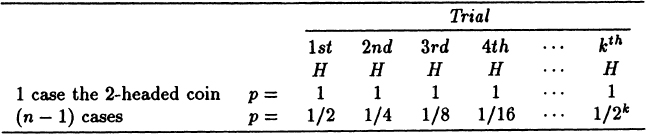
In particular, for k (heads in a row) we have for the false coin the probability of (1/n = probability of getting the false coin)

$(1/n)(1)$

while for a good coin

$\{(n-1)/n\}\{1/2^k\}$

Let us take their ratio

$\text{false coin/(good coin)}=2^k/(n-1)$

When n is large you need a reasonably large number k of trials of tossing the chosen coin so that you can safely decide that you probably have a false coin, (you need k ~ log₂(n − 1) to have the ratio 1), and to have some safety on your side you need more than that number. How many tosses you want to make depends on how much risk you are willing to take and how costly another trial is; there can be no certainty.

Example 1.9–5    No Information

You draw a card from a well shuffled deck, but do not look at it. Without replacing it you then draw the second card. What is the probability that the second card is the ace of spades?

The probability that the first card was the ace of spades is 1/52 and in that case you cannot get it on the second draw. If it was not the ace of spaces, probability 51/52, then your chance of the ace on the second draw is 1/51. Hence the total probability is

$(1/52)(0)+(51/52)(1/51)=1/52$

and it is as if the first card had never been drawn! You learned nothing from the first draw so it has no effect on your estimate of the outcome of the second draw.

Evidently, by a slight extension to a deck of n cards and induction on the number of cards removed from the deck and not looked at, then no matter how many cards (less than n) were drawn and not looked at, the probability of then drawing any specified card is 1/n.

In most situations if one person knows something and uses it to compute a probability then this probability will differ from that computed by another person who either does not have that information or does not use it. See also Example 1.9–8.

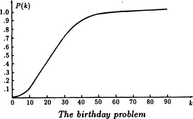
Example 1.9–6    The Birthday Problem

The famous birthday problem asks the question, “What is the fewest number of people that can be assembled in a room so there is a probability greater than 1/2 of a duplicate birthday.”

We, of course, must make some assumptions about the distribution of birthdays throughout the year. For convenience it is natural to assume that there are exactly 365 days in a year (neglect the leap year effects) and assume that all birthdays are equally likely, namely each date has a probability 1/365. We also assume that the birthdays are independent (there are no known twins, etc.).

There are the cases of one pair of duplicate birthdays, two pairs of duplicate birthdays, triples, etc.—many different cases to be combined. This is the typical situation where you use the complement probability approach and compute the probability that there are no duplicates. We therefore first compute the complement probability Q(k) that k people have no duplicate birthdays.

To find Q(k), the first person can be chosen in 365 equally likely ways—365/365 is the correct probability of no duplication in the selection of only one person. The second person can next be chosen for no duplicate in only 364 ways—with probability 364/365. The third person must not fall on either of the first two dates so there are only 363 ways, the next 362 ways, … and the k^th in 365 − (k − 1) = 365 − k + 1 ways. We have, therefore, for these independent selections

$\begin{array}{ll}P(k)\hfill & =1-Q(k)\hfill \\ \hfill & =1-(365/365)(364/365)\dots [(365-k+1)/365]\hfill \end{array}$

To check this formula consider the cases: (1), P(365) ≠ 1; (2), Q(366) = 0, hence, as must be, P(366) = 1, there is certainly at least one duplicate! Another check is k = 1 where Q(1) = 1, hence P(1) = 0 as it should. Thus the formula seems to be correct.

Alternately, to compute Q(k) we could have argued along counting lines. We count the number of cases where there is no duplicate and divide by the total number of possible cases. The first person can be chosen in 365 ways, the second (non duplicate) in 364 ways, the third in 363 ways, … the k^th in 365 − k + 1 ways. The total number of ways (the size of the product space) is 365^k and we have the same number for Q(k), the complement probability.

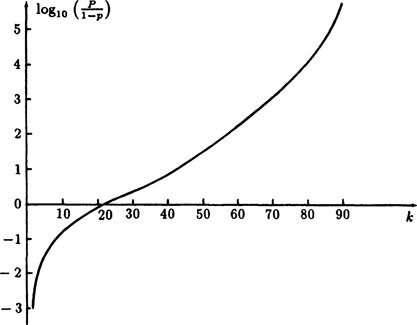
It is difficult for the average person to believe the results of this computation so we append a short table of P(k) at a spacing of 5 and display on the right in more detail the part where P(k) is approximately 1/2.

TABLE 1.9–1

Table of P(k) for selected values

P(k)	log10 P/(1 – P)	P(k)
P(5) = 0.02714	−1.5541	P(21) = 0.44369
P(10) = 0.11695	−0.87799	P(22) = 0.47570
P(15) = 0.25290	−0.47043	P(23) = 0.50730
P(20) = 0.41144	−0.15545	P(24) = 0.53834
P(25) = 0.56870	+0.12010
P(30) = 0.70632	0.38113
P(35) = 0.81438	0.64220
P(40) = 0.89123	0.91348
P(45) = 0.94098	1.2026
P(50) = 0.97037	1.5152
P(55) = 0.98626	1.8560
P(60) = 0.99412	2.2281
P(65) = 0.99768	2.6335
P(70) = 0.99916	3.0754
P(75) = 0.99972	3.5527
P(80) = 0.99991	4.0457
P(85) = 0.99998	4.6990
P(90) = 0.99999	4.9999

The result that for 23 people (and our assumptions) the probability of a duplicate birthday exceeds 1/2 is surprising until you remember that any two people can have the same birthday, and it is not just a duplicate of your birthday. There are C(n, 2) = n(n − 1)/2 pairs of people each pair with a probability of approximately 1/365 of a coincidence, hence the average number of coincidences is, for n = 28,

$(28\times 27)/2(365)=1.0356\dots$

hence again the result is reasonable, but see Example 1.9–7.

FIGURE 1.9–1

The curve of this data is plotted in Figure 1.9–1 and,shows a characteristic shape for many probability problems; there is a slow beginning, followed by a steep rise, and then a flattening at the end. This illustrates a kind of “saturation phenomenon”—at some point you pass rapidly from unlikely to very likely. In Figure 1.9–2 we plot log{P/(1 − P)} to get a closer look at the two ends of the table.

FIGURE 1.9–2

The sequence of numbers we have introduced has the convenient notation of descending factorials

${(n)}_k=n(n-1)(n-2)\cdots (n-k+1)$

(1.9–1)

which is the product, beginning with n, of k successive terms each 1 less than the preceeding one and ends with n − (k − 1).

Example 1.9–7    The General Case of Coincidences

If we draw at random from a collection of n distinct items, and replace the drawn item each time before drawing again, what is the probability of no duplicate in k trials?

The reasoning is the same as in the previous problem. The first has a probability of no duplicate is n/n, the second for no duplicate is (n − 1)/n, and so on to the k^th (where you must avoid all the previous k − 1 samples) which is (n − k + 1)/n; hence we have the probability for all k independent trials

$\begin{array}{ll}{Q}_n(k)\hfill & =n(n-1)(n-2)\dots (n-k+1)/n^k={(n)}_k/n^k\hfill \\ \hfill & =n!/n^k(n-k)!\hfill \\ \hfill & =[1-1/n][1-2/n]\dots [1-(n-k+1)/n]\hfill \end{array}$

The numerator in the top of these three equations is the falling (descending) factorial with exactly k terms. For n = 365 we have the Q(k) of the birthday problem.

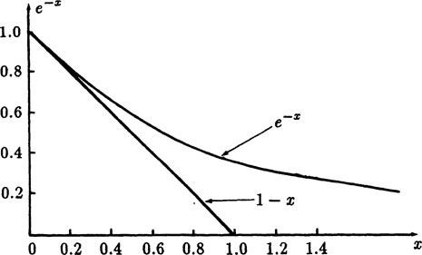
To evaluate this expression easily we use the third line and an inequality from Appendix 1.B, namely that for x > 0

$1-x<e^{-x}$

on each term of the above product. This gives

$Q_n(k)<\exp [-\{1/n+2/n+\cdots +(k-1)/n\}]=\exp [-k(k-1)/2n]$

For the probability of the bound to be 1/2 we get

$\begin{array}{l}\mathit{ln\hspace{0.17em}}2=k(k-1)/2n\\ k^2-k-2n\mathit{ln\hspace{0.17em}}2=0\end{array}$

For the birthday problem n = 365, and we solve the quadratic to get 23.000 within roundoff.

To get a feeling for the function y(k) = (n)_k/n^k we look for the place where it rises most steeply. This occurs close to where the second central difference is 0, that is where

$y(k+1)-2y(k)+y(k-1)~0$

We can immediately factor out the y(k) to get (remember k > 0)

$\begin{array}{l}y(k)[(n-k)/n-2+n/(n-k+1)]=0\\ {(n-k)}^2+n-k-2n^2+2nk-2n+n^2=0\\ k^2-k-n=0\\ k=\{1\pm \sqrt{(1+4n)}\}/2=\{1+\sqrt{(4n+1)}\}/2\\ ~\sqrt{n}+1/2\end{array}$

For the birthday problem n = 365, and we have the approximate place of steepest rise is

$k~\sqrt{n}+1/2=19.10+1/2=19.6$

and this indeed we see in Table 1.9–1, and Figure 1.9–1 where the steepest rise precedes the 50% point of k = 23.

Example 1.9–8    The Information Depends on Your State of Knowledge

There is (was?) a TV game in which you guess behind which of three curtains the prize you might win is placed. Your chance of success is 1/3 because of the obvious assumption that there is no pattern in the placing of the prize (otherwise long term watchers would recognize it). The next step is that the host of the show pulls back a curtain, other than the one you indicated, and reveals that there is no prize there. You are then given the chance of changing your choice for the payment of a fixed sum. What should you do?

Your action logically depends on what you think the host knows and does. If you assume that the host does not know where the prize is and draws the curtain at random (one of the two left) then the sample space has only six possibilities. If we assume that the prize is behind A but you do not know which is A, (hence any pattern you might use is equivalent to your choosing A, B or C at random), then the sample space (you, host) is

$\begin{array}{llllll}(A,B)\hfill & (A,C)\hfill & (B,A)\hfill & (B,C)\hfill & (C,A)\hfill & (C,B)\hfill \end{array}$

each with probability 1/6. In the case we are supposing, the host’s curtain reveals no prize and this eliminates the points (B, A) and (C, A) from the sample space, so that your probability is now

$P=2(1/6)/\{1-1/3\}=1/(3-1)=1/2$

Your probability passed from 1/3 to 1/2 because you learned that the prize was not in one of the places and hence it is in one of the remaining two places.

But it is unlikely that the host would ever pull the curtain with the prize behind it, hence your more natural assumption is that he does not pull the curtain at random, but rather knows where the prize is and will never draw that one. Now the situation is that if you happened to pick A (with probability 1/3) the host will pull a curtain at random and the two cases

$\begin{array}{ccc}(A,B)& \text{and}& (A,C)\end{array}$

will each have a probability 1/6. But if you pick either B or C then the host is forced to choose the other curtain behind which the prize is not located. Your choices B or C each remain of probability 1/3. Although you now know that the prize is either behind your choice or the other one you have learned nothing since you knew that the curtain drawn would not show the prize. You have no reason to change from you original choice having probability of 1/3. Hence the other curtain must have probability 2/3.

If this seems strange, let us analyse the matter when the host chooses with a probability p the curtain that does not have the prize. Then the host chooses the curtain with the prize q = 1 − p. Now the cases in the sample space are:

$\begin{array}{l}p(AB)=1/6=p(AC)\\ p(BA)=(1-p)/3=p(CA)\\ p(BC)=p/3=p(CB)\end{array}$

As a check we see that the total probability is still 1. The fact that the curtain was drawn and did not reveal the prize means that the cases p(BA) and p(CA) are removed from the sample space. So now your probability of winning is

$\begin{array}{l}P=\{p(AB)+p(AC)\}/\{1-p(BA)-p(CA)\}=\{1/3\}/\{1-2(1-p)/3\}\\ =\{1/3\}/\{1/3+2p/3\}=1/\{1+2p\}\end{array}$

We make a short table to illustrate things and check our understanding of the situation.

p	P	meaning
1	1/3	Host never reveals the prize.
1/2	1/2	Host randomly reveals the prize.
0	1	Host must reveal it if it can be done and since he did not you must have won.

Hence what you think the host does influences whether you should switch your choice or not. The probabilities of the problem depend on your state of knowledge.

It should be evident from the above Examples that we need to develop systematic methods for computing such things. The patient reasoning we are using will not work very well in larger, more difficult problems.

Exercises 1.9

1.9–1 Consider the birthday problem except that you ask for duplicate days of the month (assume that each month has exactly 30 days). Ans. P(7) = 0.5308

1.9–2 If there are only 10 possible equally likely outcomes how long will you expect to wait until the probability of a duplicate is > 1/2? Assume that the trials are independent. Make the complete table. Ans. P(1) = 0, P(2) = .1, P(3) = .28, P(4) = .496, P(5) = .6976, P(6) = .8488, P(7) = .93952, P(8) = .981856, P(9) = .9963712, P(10) = .99963712.

1.9–3 There are three children in a family and you observe that a randomly chosen one is a boy, what is the probability that the other two children have a common sex?

1.9–4 There is a box with four drawers. The contents are respectively GGG,GGS,GSS, and SSS.You pick a drawer at random and a coin at random. The coin is gold. What is the probability that there is another gold coin in the drawer? That a second drawing from the drawer will give a gold coin? Ans. 5/6, 2/3.

1.9–5 Generalize the previous problem to the case of n coins per drawer. Find the probability that the first two coins drawn are both gold. Ans. 2/3

1.9–6 If you suppose that a leap year occurs exactly every fourth year, what is the probability of a person being born on Feb. 29?

1.9–7 In Example 1.9–6 use y” = 0(y” = second derivative) in place of the second difference to obtain a similar result.

1.9–8 You have 2n pieces of string hanging down in your hand and you knot pairs of them, tying at random an end above with and end above and below with below, also at random. What is the probability that you end up with a single loop? [Hint:Knotting pairs at random above has no effect on the problem and you are reduced to n U shaped pieces of string. Proceed as in the birthday problem with suitable modifications (of course)].

1.9–9 From a standard deck k cards are drawn at random. What is the probability that no two have the same number? Ans. 4^k(13)_k/(52)_k

1.9–10 One card is drawn from each of two shuffled decks of cards. What is the probability:

1.  the card from the first deck is black?

2.  at least one of the two cards is black?

3.  if you know that at least one is black, that both are black?

4.  that the two cards are of opposite color?

1.9–11 In Appendix 1.B get one more term in the approximation for 1 – x using e^-x exp(—x²/2).

1.9–12 Apply Exercise 1.9–11 to Example 1.9–7.

1.9–13 There are w white balls and b black balls in an urn. If w + b − 1 balls are drawn at random and not looked at what is the probability that the last ball is white? Ans. w/(w + b).

1.9–14 Show that a bridge hand can be easily described by 64 bits. [Hint-give three 4 bit numbers to tell the number of cards in spades, hearts, and diamonds (the number of clubs is obvious then) and then list the 13 card face values in the suits. The minimum representation is much harder to convert to and from the hand values.]

1.10  Critique of the model

Let us review this model of probability. It uses only the simple concepts of symmetry and interchangeability to assign a probability measure to the finite number of possible events. The concept of the sample space is very useful, whether we take the entire sample space, which may often be built up by constructing the product space from the simpler independent sample spaces, or take some subspace of the sample space.

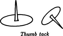
The model of equally likely situations, which is typical of gambling, is well verified in practice. But we see that all probabilities must turn out to be rational numbers. This greatly limits the possible applications since, for example, the toss of a thumb tack to see if the point is up or it is on its side (Figure 1.10–1) seems unlikely to have a rational number as its probability. Furthermore, there are many situations in which there are a potentially infinite number of trials, for example tossing a coin until the first head appears, and so far we have limited the model to finite sample spaces. It is therefore clear that we must extend this model if we are to apply probability to many practical situations; this we will do in subsequent chapters beginning with Chapter 4.

FIGURE 1.10–1

It is difficult to quarrel with this model on its own grounds, but it is still necessary to connect this model with our intuitive concept of probability as a long term frequency of occurrence, and this we will do in the next chapter where we develop some of the consequences of this model that involve more mathematical tools. The purpose of separating the concepts of probability from the mathematics connected with it, is both for philosophical clarity (which is often sadly lacking in many presentations of probability) and the fact that the mathematical tools have much wider applications to later models of probability that we will develop.

Remember, so far we have introduced a formal measure of probability based on symmetry and it has no other significant interpretation at this point. We used this measure of probability to show how to compute the probabilites of more complex situations from the uniform probability of the sample space. As yet we have shown no relationship to the common view that probability is connected with the long term ratio of successes to the total number of trials. Although very likely you have been interpreting many of the results in terms of “frequencies,” probability is still a measure derived from the symmetry of the initial situation. The frequency relationship will be derived in Section 2.8.

Appendix 1.A Bounds on Sums

We often need to get reasonable bounds on sums that arise in probability problems. The following is a very elementary way of getting such bounds, and they are often adequate.

Suppose we have the continuous function

$y=f(x)$

and want to estimate the sum

$S(N)={\displaystyle \sum _{n=1}^{N}f(n)}$

We also suppose that the second derivative f″(x) is of constant sign.

Suppose first that

$f^{″}(x)>0$

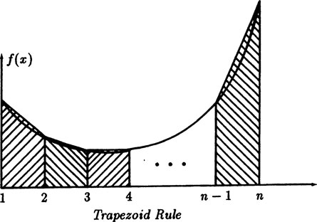
The trapezoid rule overestimates the integral, Figure 1.A–1,

${\displaystyle {\int }_1^{N}f(x)dx\le \frac{1}{2}f(1)+f(2)+\cdots +\frac{1}{2}f(N)}$

Hence add (1/2)[f(1) + f(0)] to both sides to get

${\displaystyle {\int }_1^{N}f(x)dx+\{f(1)+f(N)\}/2\le {\displaystyle \sum _1^{N}f(n)}}$

(1.A–1)

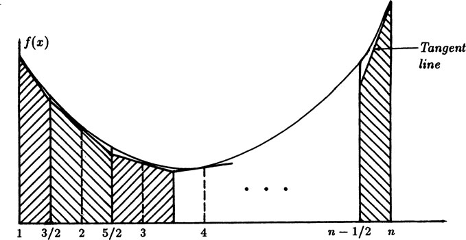
On the other hand the midpoint integration formula underestimates the integral. We handle the two half intervals at the ends by fitting the tangent

FIGURE 1.A–1

line at the ends (see Figure 1.A–2).

$\begin{array}{l}{\displaystyle {\int }_1^{N}f(x)dx}\ge {\displaystyle {\int }_1^{3/2}\{f(1)+(x-1)f^{\prime }(1)\}dx}\\ +f(2)+f(3)+\cdots f(N-1)+{\displaystyle {\int }_{N-1/2}^N\{f(N)+(x-N)f^{\prime }(N)\}dx}\\ \ge f(1)/2+{(1/2)}^2{f}^{\prime }(1)/2+{\displaystyle \sum _2^{N-1}f(n)+f(N)/2-{(1/2)}^2{f}^{\prime }(N)/2}\end{array}$

FIGURE 1.A–2

Rearranging things we have

${\displaystyle \sum _1^{N}f(n)}\le {\displaystyle {\int }_1^{N}f(x)dx+[f(1)+f(N)]/2+[f^{\prime }(N)-f^{\prime }(1)]/8}$

(1.A–2)

If f″(x) < 0 the inequalities are reversed.

The two bounds 1.A–1 and 1.A–2 differ by the term

$[f^{\prime }(N)-f^{\prime }(1)]/8$

(1.A–3)

Since most of the error generally occurs for the early terms you can sum the first k terms separately and then apply the formulas to the rest of the sum. Often the result is much tighter bounds since f′(1) becomes f′(k + 1) in the error term and f′(k) is generally a decreasing function of k.

We now apply these formulas to three examples which are useful in practice. First we choose f(x) = 1/x We have f′(x) = − 1/x² and $f^{″}(x)=2/x^3>0$. The indefinite integral is, of course, merely In N. Hence from 1.A–1 and 1.A–2 we have for the harmonic series

$\mathit{ln\hspace{0.17em}}N+(N+1)/2N\le {\displaystyle \sum _1^{N}1/n\le \mathit{ln\hspace{0.17em}}N+(N+1)/2N+(1-1/N^2)/8}$

(1.A–4)

The sum

${\displaystyle \sum _{n=1}^{N}1/n=H(N)}$

(1.A–5)

occurs frequently, hence a short table of the exact values is useful to have. Similarly, the sums

${\displaystyle \sum _{n=1}^{N}1/n^2=D(N)}$

(1.A–6)

are also useful to have. Since most of the error arises from the early terms, using these exact values and then starting the approximation formulas at the value n = 11 will give much better bounds.

A Short Table of H(N) and D(N)

N	H(N)		D(N) decimal
	fraction	decimal
1	1	1.00000	1.00000
2	3/2	1.50000	1.25000
3	11/6	1.83333	1.36111
4	25/12	2.08333	1.42361
5	137/60	2.28333	1.46361
6	147/60	2.45000	1.49133
7	1089/420	2.59285	1.51180
8	2283/840	2.71786	1.52742
9	7129/2520	2.82897	1.53977
10	7391/2520	2.92897	1.54977

At N = 10 the limits of the bounds are 2.85207 < H(N) < 2.97634. The limiting value of D(N) = π²/6 = 1.64493….

There is also a useful analytic expression for H(N) which we will not derive here, namely

$H(N)=\mathit{ln\hspace{0.17em}}N+\gamma +1/2N-1/12N^2+1/120N^3+\cdots$

(1.A–7)

where γ = 0.57721 56649… is Euler’s constant. If we use this formula through the 1/N² term for N = 10 we get H(10) = 2.92897 which is the correct rounded off number.

For the second example we use $f(x)=1/x^2$, for which $f^{\prime }(x)=-2/x^3$ and $f^{″}(x)=6/x^4>0$. The formulas give

$3/2-1/N+1/2N^2\le {\displaystyle \sum _1^{N}1/n^2\le 3/2-1/N+1/2N^2+(N^3-1)/N^3}$

(1.A–8)

For the third example we pick f(x) = ln x, for which f′(x) = 1/x and $f^{″}(x)=-1/x^2<0$. Hence the inequalities are reversed. We get for the integral (using integration by parts)

${\int }_1^N\mathit{ln\hspace{0.17em}}xdx=N\mathit{ln\hspace{0.17em}}N-N+1$

and for the formula for the bounds

$\begin{array}{ll}N\mathit{ln\hspace{0.17em}}N-N+1+(1/2)\mathit{ln\hspace{0.17em}}N\hfill & \ge {\displaystyle \sum _{n=1}^N\mathit{ln\hspace{0.17em}}n=\mathit{ln\hspace{0.17em}}N!}\hfill \\ \hfill & \ge N\mathit{ln\hspace{0.17em}}N-N+(1/2)\mathit{ln\hspace{0.17em}}N+7/8+1/8N\hfill \end{array}$

Dropping the last term on the right strengthens the inequality and taking exponentials we get the more usual form for the factorial function

$N^{N+1/2}{e}^{-N}e\ge N!\ge N^{N+1/2}{e}^{-N}{e}^{7/8}$

(1.A–9)

These bounds may be compared with the asymptotic form of Stirling’s factorial approximation

$N!=N^N{e}^{-N}\sqrt{(2\pi N)}$

(1.A–10)

Note that e = 2.71828, $\sqrt{(2\pi )}$, and e^7/8 = 2.39887 (all to five decimal places).

Bounds are almost essential in “deep” computations where approximations are combined in many ways. On the other hand for “shallow” computations Stirling’s and other approximations are often very useful.

A particularly simple approximation is the midpoint formula

${\displaystyle {\int }_{a-1/2}^{b+1/2}f(x)dx}~{\displaystyle \sum _{n=a}^{n=b}f(n)}$

(1.A–11)

In the three earlier cases we get for f(x) = 1/x

${\displaystyle \sum _1^{N}1/n~\mathit{ln\hspace{0.17em}}(2N+1)}$

(1.A–12)

for f(x) = 1/x² we get

${\displaystyle \sum _1^{N}1/n~4N/(2N+1)}$

(1.A–13)

and for f(x) = ln x we get

${\displaystyle \sum _1^N\mathit{ln\hspace{0.17em}}n~(N+1/2)\mathit{ln\hspace{0.17em}}(N+1/2)-N+(1/2)\mathit{ln\hspace{0.17em}}2}$

(1.A–14)

Taking exponentials we get the formula

$n!~{(N+1/2)}^{N+1/2}{e}^{-N}\sqrt{2}$

(1.A–15)

FIGURE 1.B-1

Appendix 1.B A Useful Bound

If we compute the tangent line to the curve

$y(x)=e^{-x}=\exp (-x)$

at x = 0 we get for the first derivative

$y^{\prime }(x)=e^{-x}$

hence

$y^{\prime }(0)=-1$

and the tangent line is

$\begin{array}{l}y(x)-1=(-1)(x-0)\\ y=1-x.\end{array}$

Since y”(x) = exp(-x) > 0 we deduce, or else from a sketch of the curve Figure 1.B-1,

$e^{-x}=\exp (-x)\ge 1-x$

(1.B-1)