2

Some Mathematical Tools

2.1    Introduction

C. S. Peirce (1839–1914) observed [N, p.1334] that:

“This branch of mathematics [probability] is the only one, I believe, in which good writers frequently get results entirely erroneous. In elementary geometry the reasoning is frequently fallacious, but erroneous conclusions are avoided; but it may be doubted if there is a single extensive treatise on probabilities in existence which does not contain solutions absolutely indefensible. This is partly owing to the want of any regular methods of procedure; for the subject involves too many subtleties to make it easy to put problems into equations without such aid.”

There were, I believe, two additional important reasons for this state of affairs at that time and to some extent even now; first there was a lack of clarity on just what model of probability was being assumed and of its known faults, and second, there was a lack of intuition to protect the person from foolish results. Feller [F, p.67] is quite eloquent on this point. Thus among the aims of this book are to provide: (1) careful discussions of the models assumed and any approach adopted; (2) the use of “regular methods” in preference to trick methods that apply to isolated problems; (3) the deliberate development of intuition by the selection of problems, (4) the analysis of the results, and (5) the systematic use of reasonableness tests of equations and results. By these methods we hope to mitigate the statement of C. S. Peirce just quoted.

In the previous chapter we created a probability model based on symmetry, and noted that it could only give rational values for the assignment of the probability to the events, and that all the elementary events had the same probability. We will later be able to handle a wider range of probabilities, namely any real number between 0 and 1 (and complex numbers in Section 8.13) as well as nonuniform probability distributions, hence we will now assume this use and not have to repeat the development of the mathematical tools for handling probability problems. The relevant rules we have developed apply to these nonrational probabilities as can be easily seen by rereading the material.

We saw that the central problem in computing the probability of a complex event is to find all the equally likely elementary successful events in the sample space (those that meet the given conditions), or else the failing events (those that do not), count the successes, or failures, and then divide by the size of the whole sample space. Instead of counting the successes in the uniform sample space and dividing by the total we can add the probabilities of all the individual successes; this is equivalent to assigning to each point in the uniform sample space the probabilty l/(total number of points in the sample space).

If the probabilities are not uniform in the sample space we cannot simply count and divide by the total, but as just noted we must add the probabilities of the individual successful events to get the total probability to assign to the complex event since the probability of the sum is additive (we pick our sample space points to be independent hence the probability of a complex event involving sums of points is the sum of the probabilities of its independent parts). Since the total probability is 1 there is no need to divide by the sum of the probabilities (which is 1).

We also saw that the probabilities assigned to the points in the product space could often be found as the product of the probabilities of the basic events that make up the corresponding point in the product space. We adopt a colorful language to use while computing probability problems; we say, for example, “Select at random…” and mean “Count the number of successes (in the case of a uniform probability assignment).” As an example, “Select a random day in a year of 365 days.” means that since any day of the year meets this condition there are 365 choices, and the corresponding probability that you select a (some) day is 365/365 = 1. The probability of getting a specific day if it is named in advance is, of course, 1/365. If we want to select at random, from the possible 365 days in a year, a day that falls in a certain month of 30 days, then there are only 30 successful possible selections, and the corresponding probability is 30/365 = 6/73. We say that we can select at random a day in the year that falls in the given month in 30 successful ways, hence with probability of 30/365.

The language “select at random” enables us to pass easily from the uniform probability spaces to nonuniform probability spaces, since in both cases we use the same colorful language and the results are the same; of course for the nonuniform case we must add the probabilities of the successes. A “random selection” is only a colorful way of talking, and when the word “random” is used without any modifier it implies that the probability assignment is uniform.

The purpose of this chapter is to introduce the main tools for computing simple probability problems which have a finite, discrete sample space, and to begin the development of uniform methods of solution as well as the development of your intuition. This Chapter also shows a connection to the frequency approach to probability. Chapter 3 will further develop, in a more systematic way, the mathematical tools needed for finite sample spaces. There is a deliberate separation between the model of probability being assumed, the concepts needed for solving problems in that area, and the mathematical tools needed for their solution.

2.2    Permutations

You have already seen that the main difficulty, in simple probability problems, is to count the number of ways something can be done. Hence we begin with this topic (actually partially repeat).

Suppose you have a collection of n distinct things (unspecified in detail, but whatever you care to think about). From these n items you then select at random k times, replacing the selected item each time before the next selection. The sample space is the product space n × n × n … × n (k times) with exactly (we “star” important equations)

$n^k$

(2.2–1)*

items in the product space. This is called sampling with replacement. The probability distribution for a random selection is uniform, hence each item in the sample space will have the probability 1/n^k.

Again, suppose you have n things and sample k times, but now you do not replace the sampled items before the next selection. When the order of selection is important then we call the selection without replacement a permutation. The number of these permutations is written as

$P(n,k)$

and is called “the permutation of n things taken k at a time.” To find the numerical value for a random (uniform) selection we argue as before, (Examples 1.9–6 and 1.9–7); the first item may be selected in n ways, the second distinct item in n − 1 ways, the third in n − 2 ways, and the k^th in n − k + 1 ways. The product space is of size

$P(n,k)=n(n-1)(n-2)\dots (n-k+1)={(n)}_k$

(2.2–2)*

where (n)_k is the standard notation for the falling factorial, (see Equation 1.9-1). By our method of selection of the individual cases in the (n)* are uniformly probable hence we add the number of cases to get the P(n,k).

To partially check this formula we note that when k = 1 the answer is correct, and when k = n + 1 we must have zero since it is impossible to select n + 1 items from the set of n items.

A useful bound on P(n, k) can be found by multiplying and dividing the right hand side of (2.2–2) by n^k

$P(n,k)=n^k(1)(1-1/n)(1-2/n)\dots (1-(k-1)/n)$

and then using the result in Appendix l.B (see also Example 1.9–7)

$1-x\le e^{-x}$

for each factor (1 – i/n), (i = 1,2,…,k − 1). Summing this arithmetic progression in the exponent

$-\{1/n+2/n+\cdots +(k-1)/n\}=-k(k-1)/2n$

we get the result

$P(n,k)\le n^{k}epx\{-k(k-1)/2n\}$

(2.2–3)

For an alternate proof that all the P(n, k) individual cases are uniformly probable note that from the sample space of all possible choices of k items, which we saw (2.2–1) was uniformly probable and of size n^k, we excluded all those which have the same item twice or more, and we deduced that there are exactly P(n, k) such points left in the sample space. Since a random choice leads to a uniform distribution in the original product space, the distribution is still uniform after the removal of the samples with duplicates (see Example 1.9–1, the gold coin problem). All the permutations in the P(n,k) are equally likely to occur when the items are selected at random. The exponential gives an estimate of the modifying factor for the number of terms in going from the sample space of sampling with replacement to sampling without replacement.

The expression P(n, k) is the beginning of a factorial. If we multiply both numerator and denominator by (n − k)! the numerator becomes n!, and we have

$P(n,k)=\frac{n!}{(n-k)!}$

(2.2–4)*

as a useful formula for the permutations of n things taken k at a time. Recall that by convention 0! = 1 and that P(n,n) = n!. We need also to observe that when k = 0 we have

$P(n,0)=\frac{n!}{n!}=1={(n)}_0$

(2.2–5)

At first this seems like a curious result of no interest in practice, but when programming a descending factorial on a computer you initialize the iterative loop of computation for P(n,k) with P(n,0) = 1; then and only then will each cycle of the computing loop give the proper number and be suitably recursive.

Example 2.2–1    Arrange Three Books on a Shelf

In how many ways can you arrange 3 books on a shelf out of 10 (distinct) books? Since we are assuming that the order of the books on the shelf matters (the word “arrange”), we have

$P(10,3)=10\times 9\times 8=720$

ways.

Example 2.2–2    Arrange Six Books on a Shelf

In how many ways can you arrange on a shelf 6 books out of 10 (distinct) books? You have

$P(10,6)=10\times 9\times 8\times 7\times 6\times 5=151,200$

possible ways of arranging them.

Example 2.2–3    Arange Ten Books on a Shelf

In how may ways can you arrange on a shelf a set of 10 distinct books? You have

$P(10,10)=10!=3,628,800$

and you see how fast permutations can rise as the number of items selected increases. The Stirling approximation from Appendix l.A gives 10! ~ 3,598,695.6 and the ratio of Stirling to true is 0.99170.

Example 2.2–4    Two Out of Three Items Identical

Suppose you have three items, two of which are indistinguishable. How many permutations can you make? First we carefully write out the sample space with elements a₁, a₂, b supposing we have three distinct elements.

$\begin{array}{l}{a}_1{a}_{2}b\\ a_{1}b{a}_2\\ a_2{a}_{1}b\\ a_{2}b{a}_1\\ b{a}_1{a}_2\\ b{a}_2{a}_1\end{array}$

Now if a₁ and a₂ are indistiguishable then items on lines 1 and 3, 2 and 4, and 5 and 6 are each the same; the reduction of the sample space from 6 to 3 is uniform. The following formula gives the proper result

$3!/2=6/2=3$

Example 2.2–5    Another Case of Identical Items

In permutation problems there are often (as in the previous Example) some indistinguishable items. For example you may have 7 items, a, a, a, b, b, c, d. How many permutations of these 7 items are there?

We again attack the problem by throwing it back on known methods; we first make the 3 a’s distinct, calling them a₁, a₂, a₃, and similarly the 2 b’s are now to be thought of as b₁ and b₂. Now we have P(7,7) = 7! permutations. But of these there are P(3,3) = 3! permutations which will all become the same when we remove the distinguishing subscripts on the a’s, and this applies uniformly throughout the sample space, hence we have to divide the number in the total sample space by P(3,3) = 3!, Similarly, for the b’s we get P(2,2) = 2! as the dividing factor. Hence we have, finally, the sample space of distinct permutations

$\frac{7!}{3!2!1!1!}=7\times 6\times 5\times 4/2=420$

as the number of permutations with the given repetitions of indistinguishable items (we have put 1! twice in the denominator for symmetry and checking reasons, 3 + 2 + 1 + 1 = 7). Since the reduction from distinct items in the original permutation sample space to those in the reduced permutation space is uniform over the whole sample space, the probabilities of the random selection of a permutation with repetitions are still uniform. If this is not clear see the previous Example 2.2–4.

The general case is easily seen to follow from these two special cases, Examples 2.2–4 and 2.2–5. If we have n₁ of the first kind, n₂ of the second, …, and n_k of the k^th, and if

$n_1+n_2+\cdots +n_k=n$

then there are

$\frac{n!}{n_1!n_2!\dots n_k!}=C(n;n_1,n_2,\dots n_k)$

(2.2–6)*

permutations all of equal probability of a random selection.

These numbers, C(n;n₁, n₂,…n_k), are called the multinomial coefficients in the expansion

${(t_1+t_2+t_3+\cdots +t_k)}^n$

They occur when you expand the multinomial and select the term in t₁ to the power n₁, t₂ to the power n₂,…t_k to the power n_k, and then examine its coefficient. The coefficient is the number of ways that this combination of powers can arise; this coefficient is the number of permutations with the given duplication of items. Note that if n₁ = k and all the other n_i = 1, then this is P(n, k).

This formula applies to the case when all the terms are selected. If only a part of them are to be selected then it is much more complex in detail, but the ideas are not more complex. You have to eliminate the “over counting” that occurs when the items are first thought of being distinct because the reductions are not necessarily uniform over the sample space. We will not discuss this further as it seems to seldom arise in practice. Simple cases can be done by merely listing the sample space.

Exercises 2.2

2.2–1 How many arrangements on a platform can be made when there are 10 people to be seated?

2.2–2 How many arrangements can you make by selecting 3 items from a set of 20? Ans. 570.

2.2–3 In a standard deck of 52 cards what is the probability that on drawing two cards you will get the same number (but not suit)? Ans. 3/51.

2.2–4 In drawing three cards what is the probability that all three are in the same suit? Ans. (12/51)(11/50) = 22/425.

2.2–5 In drawing k ≤ 13 cards what is the probability that all are in the same suit?

2.2–6 Show that P(n, k) = nP(n − 1, k − 1).

2.2–7 You are to place 5 distinct items in 10 slots; in how many ways can this be done?

2.2–8 Tabulate P(10, k)/10^k for k = 0,1,… 10. Ans. 1, 0.9, 0.72, 0.504, etc.

2.2–9 Estimate P(100,10) using (2.2–3).

2.2–10 Estimate P(100,100) using both (2.2–3) and Stirling’s formula (l.A–10). Explain the difference.

2.2–11 Given a circle with n places on the circumference, in how many ways can you arrange k items? Ans. P(n,k)/n

2.2–12 If in 2.2–11 you also ignore orientation, and n is an odd number, in how many ways can you arrange the k items?

2.2–13 Using all the letters how many distinct sequences can you make from the letters of the word “success”? Ans. 420.

2.2–14 Using all the letters how many distinct sequences can you make from the letters of the word “Mississippi”? Ans. C(11;4,4,2,1) = 4950.

2.2–15 Using all the letters how many distinct sequences can you make from the letters of the word “Constantinople”?

2.2–16 How many distinct three letter combinations can you make from the letters of Mississippi? Ans. 38.

2.2–17 How many four letter words can you make from the letters of Mississippi?

2.2–18 If an urn has 7 w (white) and 4 b (black) balls show that on drawing two balls Pr{w, w) = 21/55, Pr{b, w} = 14/55 = Pr{w, b}, Pr{b, b} = 6/55.

2.2–19 If you put 5 balls in three bins at random what is the probablity of exactly 1 empty bin?

2.2–20 There are three plumbers in town and on one day 6 people called at random for a plumber. What is the probability 3, 2 or only one plumber was called? Show that the Pr{3,2,1} = 20/343.

2.2–21 Discuss the accuracy of (2.2–3) when k is small with respect to n. When k is large.

2.3    Combinations

A combination is a permutation when the order is ignored. A special case of the multinomial coefficients occurs when there are only two kinds of items to be selected; they are then called the binomial (bi = two, nomial = term) coefficients C(n,k). The formula (2.2–6) becomes

$C(n,k)=\frac{n!}{k!(n-k)!}=C(n,n-k)$

(2.3–1)*

where there are k items of the first kind (selected) and n – k items of the other kind (rejected). We use the older notation C(n,k) in place of the currently popular notation

$\left(\begin{array}{l}n\\ k\end{array}\right)$

because: (1) it is easier to type (especially for computer terminals), (2) does not involve a lot of special line spacing when the symbol occurs in the middle of a line of type, and (3) simple computer input and output programs can recognize and handle it easily when it occurs in a formula. Note that (2.3–1) is a special case of (2.2–6) when you use k₂ = n – k₁. Note also (2.3–1) says that what you select is uniquely determined by what you leave.

Recurrence relations are easy to find for the C(n, k) and often shed more light on the numbers than an actual table of them. For the index k we have, by adjusting the factorials,

$\begin{array}{ll}C(n,k+1)\hfill & =\frac{n!}{(k+1)!(n-k-1)!}\hfill \\ \hfill & =\frac{n!(n-k)}{(k+1)k!(n-k)(n-k-1)!}\hfill \\ \hfill & =\frac{(n-k)}{(k+1)}C(n,k)\hfill \end{array}$

(2.3–2)*

Clearly the largest C(n, k) occurs around (n − k)/(k + 1) ~ 1, that is ~ (n − 1)/2.

For the index n we have the recurrence relation

$\begin{array}{ll}C(n+1,k)\hfill & =\frac{(n+1)!}{k!(n+1-k)!}=\frac{(n+1)n!}{k!(n+1-k)(n-k)!}\hfill \\ \hfill & =\frac{(n+1)}{(n+1-k)}C(n,k)\hfill \end{array}$

(2.3–3)*

The binomial coefficients C(n, k) arise from

${(t_1+t_2)}^n={\displaystyle \sum _{k=0}^{n}C(n,k)t_1^{n-k}{t}_2^k}$

In a more familiar form we have (t₁ = 1, t₂ = t)

$\begin{array}{ll}{(1+t)}^n\hfill & =1+nt+\frac{n(n-1)}{2}{t}^2+\cdots +t^n\hfill \\ \hfill & ={\displaystyle \sum _{k=0}^{n}C(n,k)t^k}\hfill \end{array}$

(2.3–4)*

where the C(n, k) are the number of ways k items can be selected out of n without regard to order. The equation (2.3–4) generates the binomial coefficients.

From this generating function (2.3–4) and the observation that

${(1+t)}^{n+1}=(1+t){(1+t)}^n$

we can equate like powers of t^k on both sides (since the powers of t are linearly independent) to get the important relation

$C(n+1,k)=C(n,k)+C(n,k-1)$

(2.3–5)*

with the side conditions that

$C(n,0)=C(n,n)=1$

An alternate derivation goes as follows. Suppose we have n + 1 items. All possible subsets of size k can be broken into two classes, those without the (n + 1)st item and those with it. Those without the (n + 1)st item total simply C(n,k), while those with it require selection only k − 1 more items, and these total C(n,k − 1). Thus we have (2.3–5).

This identity leads to the famous Pascal triangle where each number is the sum of the two numbers immediately above, and the edge values are all 1.

$\begin{array}{c}1\\ \begin{array}{cc}1& 1\end{array}\\ \begin{array}{ccc}1& 2& 1\end{array}\\ \begin{array}{cccc}1& 3& 3& 1\end{array}\\ \begin{array}{lllll}1\hfill & 4\hfill & 6\hfill & 4\hfill & 1\hfill \end{array}\\ \begin{array}{llllll}1\hfill & 5\hfill & 10\hfill & 10\hfill & 5\hfill & 1\hfill \end{array}\\ \begin{array}{lllllll}1\hfill & 6\hfill & 15\hfill & 20\hfill & 15\hfill & 6\hfill & 1\hfill \end{array}\\ \begin{array}{llllllll}1\hfill & 7\hfill & 21\hfill & 35\hfill & 35\hfill & 21\hfill & 7\hfill & 1\hfill \end{array}\\ \begin{array}{lllllllll}1\hfill & 8\hfill & 28\hfill & 56\hfill & 70\hfill & 56\hfill & 28\hfill & 8\hfill & 1\hfill \end{array}\\ \begin{array}{llllllllll}1\hfill & 9\hfill & 36\hfill & 84\hfill & 126\hfill & 126\hfill & 84\hfill & 36\hfill & 9\hfill & 1\hfill \end{array}\\ \begin{array}{lllllllllll}1\hfill & 10\hfill & 45\hfill & 120\hfill & 210\hfill & 252\hfill & 210\hfill & 120\hfill & 45\hfill & 10\hfill & 1\hfill \end{array}\\ ThePascalTriangle\end{array}$

It might be thought that to get a single line of the binomial coefficients of order n the triangle computation would be inefficient as compared to the recurrence relation (2.3–2). If we estimate the time of a fixed point multiplication as about 3 additions and a division as about two multiplications, then we see that for each term on the n^th line we have two additions, one multiplication and one division, or about 11 addition times per term. There being n − 1 terms to compute on the n^th line we have to compare this with the triangle down to the n^th line, namely n(n − 1)/2 additions. This leads to comparing

$\begin{array}{ccc}n/2& \text{with}& 11\to n=22\end{array}$

(Floating point arithmetic would give, of course, different results.) This suggests that as far as the amount of computing arithmetic is concerned it is favorable to compute the whole triangle rather than the one line you want until n = 22—which is quite surprising and depends, of course, on the actual machine times for the various operations. Symmetry reduces the amount of computation necessary by 1/2 in both approaches. One can squeeze out time for the one line approach by various tricks depending on the particular machine—the point is only that the Pascal triangle is surprisingly efficient on computers as contrasted with human computation.

From the generating function (2.3–4) we can get a number of interesting relationships among the binomial coefficients.

Example 2.3–1    Sums of Binomial Coefficients

If we set t = 1 in (2.3–2) we get

${(1+1)}^n={\displaystyle \sum _{k=0}^{n}C(n,k)=2^n}$

(2.3–6)*

In words, the sum of all the binomial coefficients of index n is exactly 2ⁿ.

If we set t = −1 we get the corresponding sum with alternating signs

${\displaystyle \sum _{k=0}^n{(-1)}^{k}C(n,k)=0}$

(2.3–7)

The alternating sum of the binomial coefficients is exactly 0 for all n. Thus the sum of all the even indexed coefficients is the same as the sum of all the odd indexed coefficients.

If we differentiate the generating function (2.3–4) with respect to t we get the identity

$n{(1+t)}^{n-1}={\displaystyle \sum _{k=1}^{n}kC(n,k)t^{k-1}}$

and when we put t = 1 we get

$n{2}^{n-1}={\displaystyle \sum _{k=1}^{n}kC(n,k)}$

(2.3–8)*

Many other useful relationships can be found by: (1) suitably picking a function of t to multiply through by, (2) differentiating or integrating one or more times, and finally (3) picking a suitable value for t. The difficulty is to decide what to do to get the identity you want. See Appendix 2.B.

Example 2.3–2    Bridge Hands

In the game of bridge each hand is dealt 13 cards at random from a deck of 52 cards with four suits. How many different sets of 4 hands are there (the order of the receiving the cards does not matter)?

Evidently we have the combination (since order in the hands does not matter)

$52!/{(13!)}^4=5.36447\text{}\dots \times {10}^{28}$

when you assume that the hands are given but not the positions around the bridge table. Thus you see the enormous number of possible bridge dealings. The Stirling approximation (A.l) gives 5.49… × 10²⁸.

Example 2.3–3    3 Out of 7 Books

A student grabs at random 3 of his 7 text books and dashes for school. If indeed the student has 3 classes that day what is the probability that the correct three books were selected?

We can argue in either of two ways. First, we can say that there are exactly C(7,3) equally likely selections possible out of the set of 7 books and that only 1 combination is correct, hence the probability is

$1/C(7,3)=3!/(7\times 6\times 5)=1/35$

We can also argue (repeating the basic derivation of the binomial coefficients) that the first book can be successfully selected in 3 out of 7 ways, hence with probability 3/7. Then the second book can independently be successfully selected in 2 out of 6 ways with probability 2/6. The third book in 1 out of 5 ways with probability 1/5. The probability of making all three independent choices correctly is, therefore,

$\left(\frac{3}{7}\right)\left(\frac{2}{6}\right)\left(\frac{1}{5}\right)=\frac{1}{35}$

which agrees with the result of the first approach.

Example 2.3–4    Probability of n Heads in 2n Tosses of a Coin

The number of ways of getting exactly n successes in 2n equally likely trials is

$C(2n,n)$

and the probability of getting this is

$C(2n,n)/2^{2n}$

because the sum of all the binomial coefficients is 2²ⁿ, by equation (2.3–6), (alternately each trial outcome has a probability of 1/2).

To get an idea of this number we apply Stirling’s formula (l.A–7). We get

$\begin{array}{ll}(2n)!\{n!n!2^{2n}\}\hfill & ~{(2n)}^{2n}{e}^{-2n}\sqrt{2\pi 2n}/\left\{n^n{e}^{-n}\sqrt{2\pi n}{n}^n{e}^{-n}\sqrt{2\pi n}{2}^{n2}\right\}\hfill \\ \hfill & ~1/\sqrt{(\pi n)}\hfill \end{array}$

Thus the exact balancing of heads and tails in 2n tosses of a coin becomes increasingly unlikely as n increases—but slowly! At n = 5, (10 tosses), this approximation gives 0.24609 vs. the exact answer 0.25231, about 1 in 4 trials.

Example 2.3–5    Probability of a Void in Bridge

What is the probability when drawing 13 cards at random from a deck of 52 cards of having at least one suit missing?

For each success we must have drawn from one of 4 decks with only 39 cards (one suit missing). Hence the probability is

$\begin{array}{ll}P\hfill & =4C(39,13)/C(52,13)=4(39!)(39!)/(26!)(52!)\hfill \\ \hfill & =0.05116\dots ~1/20\hfill \end{array}$

If your computer cannot handle a 52! then Stirling’s approximation will yield P = .05119…

Example 2.3–6    Similar Items in Bins

In how many ways can you put r indistinguishable items into n bins?

An example might be rolling r dice and counting how many have each possible face (are in each bin). The solution is simple once we realize that by adding to the r items n− 1 dividers (|) between bins; thus we are arranging n + r − 1 items

$***|**|*****|**|*******|*\dots *|***$

and this can be done in

$C(n+r-1,r)=C(n+r-1,n-1)$

different ways.

Example 2.3–7    With at Least 1 in Each Bin

If in the above distribution we have to put at least one ball into each bin then of the r balls we distribute the first n into the n bins leaving r − n balls and then proceed as before. This gives

$C(r-1,n-1)$

and we are assured of at least one in each bin.

Exercises 2.3

2.3–1 Write out the eleventh line of the Pascal triangle.

2.3–2 Use 2.3–2 to compute the eleventh line of the Pascal triangle.

2.3–3 What is the sum of the coefficients of the 11th line?

2.3–4 Compute C(10, 5) directly.

2.3–5 Find ${\displaystyle {\sum }_{k=1}^{11}kC(11,k)}$.

2.3–6 Find ${\displaystyle \sum k^{2}C(n,k)}$. Ans. $n(n+1)2^{n-2}$.

2.3–7 Find an algebraic expression for C(n, n − 1).

2.3–8 Show that C(n, n- 2) = n(n − 1)/2.

2.3–9 Show that the ratio of C(n, n − 3)/C(n, n- 2) = (n − 2)/3.

2.3–10 How many different bridge hands might you possibly get?

2.3–11 Discuss the fact that equation 2.3–1 always gives integers, that the indicated divisions always can be done.

2.3–12 For your machine find the comparative operation times and compute when the Pascal triangle is preferable to the direct computation of one line.

2.3–13 Show that if there are m Democrats and n Republicans then a committee consisting of k members from each party can be selected in C(m, k) × C(n, k) = n!m!/(n − k)! (m − k)!{k!}² different ways.

2.3–14 Make a table of the probabilities of the number of heads in 6 tosses of a well balanced coin.

2.3–15 For 20 tosses (n = 10) compare the Stirling approximation for 10 heads with the exact result. Ans. Exact =.176197, Est. =.178412.

2.3–16 What is the probability of a bridge hand having no cards other than 2, 3, 4, 5, 6, 7, 8, 9 and 10? Ans. .003639….

2.3–17 Find the sum of the terms of the form k³C(n, k).

2.3–18 Compute ${\displaystyle {\sum }_{k=0}^{n}C(n,k)/(n+1)}$.

2.3–19 If each of two people toss n coins what is the probability that both will have the same number of heads? (See 2.B-4) Ans. C(2n,n)/2²ⁿ. Check this for n = 1,2,3.

2.3–20 In a deck of 52 cards one black card is removed. There are then 13 cards dealt and it is observed that all are the same color. Show that the probability that they are all red is 2/3.

2.3–21 If n items are put into m cells show that the expected number of empty cells is (m − 1)ⁿ/mⁿ-1

2.3–22 If you expect 100 babies to be delivered in a hospital during the next 90 days, show that the expected number of days that the delivery room will not be in use is approximately 29.44 or about 1/3 of the time.

2.3–23 Balls are put into three cells until all are occupied. Give the distribution of the waiting time n. Ans. $(2^{n-1}-2)/3^{n-1},(n>2)$.

2.3–24 Show that the probability of a hand in bridge of all the same color is 2C(26,13)/C(52,13) = 19/(47)(43)(41)(7) = 0.000032757….

2.3–25 What is the approximate number of tosses of a coin when you can expect a 10% chance of half of the outcomes being heads?

2.4    The Binomial Distribution-Bernoulli Trials

Since the binomial distribution is so important we will repeat, in a slightly different form, much of the material just covered. Suppose that the probability of some event occurring is p, and of its not occurring is q = 1 − p. Consider n independent, repeated trials, called Bernoulli trials, in which there are exactly k successes, and of course n – k failures. What is the probability of observing exactly k successes?

To begin we suppose that the first k trials are all successes and that the rest are all failures. The probability of this event is

$ppp\dots pqqq\dots q=p^k{q}^{n-k}$

Next, consider any other particular sequence of Jfe successes whose positions in the run are fixed in advance, and n − k failures in the remainding positions. When you pick that sequence of k p’s and (n − k)q’s you will find that you have the same probability as in the first case.

Finally, we ask in how many ways the k successes and (n − k) failures can occur in a total of n trials; the answer is, of course, C(n,k). Hence when we add all these probabilities together, each having the same individual probability, we get

$P(k)=C(n,k)p^k{q}^{n-k}$

(2.4–1)*

as the probability of exactly k successes in n independent trials of probability p. This is often written as

$\begin{array}{cc}b(k;n,p)=C(n,k)p^k{q}^{n-k}& (0\le k\le n)\end{array}$

(2.4–2)*

In words, “the binomial probability of k successes in n independent trials each of probability p.” This gathers together all the C(n, k) equally likely, p^kq^n-k, individual events in the original product sample space and groups them as one term. The result is the probability of exactly k successes in n independent trials, each single trial with probability of success p.

We now have the probability distribution for b(k;n,p) as a function of the variable k. We see that this new distribution is not uniform. Even if p = 1/2 and the original sample space is uniform the grouped results are not.

There is a useful relationship between successive terms of this distribution which may be found as follows (from 2.3–2):

$\begin{array}{ll}b(k+1;n,p)\hfill & =C(n,k+1)p^{k+1}{q}^{n-k-1}\hfill \\ \hfill & =\left(\frac{n-k}{k+1}\right)\left(\frac{p}{q}\right)C(n,k)p^k{q}^{n-k}\hfill \\ \hfill & =\left(\frac{n-k}{k+1}\right)\left(\frac{p}{q}\right)b(k;n,p)\hfill \end{array}$

(2.4–3)

With this we can easily compute the successive terms of the distribution.

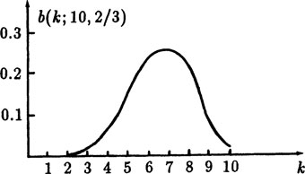
For example, suppose n = 10, and p = 2/3, then as a function of k we have (using 2.4–3)

TABLE 2.4–1

P(k)	= b(k; 10, 2/3)
P(0)	= 0.00002
P(1)	= 0.00034
P(2)	= 0.00305
P(3)	= 0.01626
P(4)	= 0.05690
P(5)	= 0.13658
P(6)	= 0.22761
P(7)	= 0.26012
P(8)	= 0.19509
P(9)	= 0.08671
P(10)	= 0.01734
Total	= 1.00000

FIGURE 2.4–1

This is the distribution of the probability function b(k; 10,2/3), see Figure 2.4–1. The total probability must be 1, of course. To show that this is true in general we observe that the generating function of b(k; n,p) can be found by

$\begin{array}{ll}{(q+pt)}^n\hfill & ={\displaystyle \sum _{k=0}^{n}C(n,k){(pt)}^k{q}^{n-k}}\hfill \\ \hfill & ={\displaystyle \sum _{k=0}^n\{C(n,k)p^k{q}^{n-k}\}{t}^k}\hfill \\ \hfill & ={\displaystyle \sum _{k=0}^{n}b(k;n,p)t^k}\hfill \end{array}$

(2.4–5)*

where the coefficient of t^k is b(k;n,p) = P(k). Now putting t = 1 we have

${(q+p)}^n=1={\displaystyle \sum _{k=0}^{n}b(k;n,p)}$

From the table we see that (within roundoff) the sum is indeed 1.

The sequence b(k; n,p) is called the binomial distribution from its obvious source. It is also called the Bernoulli distribution; it arises whenever there are n independent binary (two way) choices, each having the same probability p of success, and you are interested in exactly k successes in the n trials.

For p = 1/2 the maximum of the binomial distribution is at the middle, k = n/2, (if n is even). The approximate inflection points of this important binomial distribution for p = 1/2, (which is a discrete distribution) can be found by setting the second difference approximately equal to 0 (see 2.3–1)

$\begin{array}{l}C(n,k+1)-2C(n,k)+C(n,k-1)\\ =C(n,k)\left[\frac{n-k}{k+1}-2+\frac{k}{n-k+1}\right]~0\end{array}$

Clearing the square bracket of fractions we have

$n^2-nk-nk+k^2+n-k-2(nk-k^2+k+n-k+1)+k^2+k~0$

We arrange this in the form

$\begin{array}{l}4k^2-4nk+n^2-n-2~0\\ {(2k-n)}^2~n+2\\ k~\frac{1}{2}[n\pm \sqrt{(n+2)}]~\frac{n}{2}\pm \frac{\sqrt{n}}{2}\end{array}$

(2.4–6)*

and the inflection points for large n are symmetrically placed with respect to the position of the maximum, n/2, are at a distance approximately equal to $\sqrt{n}/2$.

Example 2.4–1    Inspection of Parts

If the probability of a defective part is 1/1000, what is the probability of exactly one defect in a shipment of 1000 items?

We reason as follows; the value from (2.4–1) is

$b(1;1000,1/1000)=C(1000,1)[(1/1000){(1-1/1000)}^{999}]=\frac{1000}{1000}{(1-1/1000)}^{1000}/(1-1/1000)$

But remembering the limit from the calculus

$\underset{n\to \infty }{\lim }{(1-1/n)}^n=1/e$

we apply this to the expression to get

$(1/e)(1-1/1000)~1/e$

(2.4–7)*

This is a passable (not very good) approximation in many situations as can be seen from the following Table 2.4–2.

TABLE 2.4–2

n	(1 − 1/n)n	Exact		Error in using 1/e
1	0	=	0
2	(1/2)2 = 1/4	=	0.25	0.178794
3	(2/3)3 = 8/27	=	0.296296	0.071583
4	(3/4)4 = 81/256	=	0.316406	0.051473
5	(4/5)5 = 1024/3125	=	0.327680	0.040199
10	(9/10)10	=	0.348678	0.019201
20	(19/20)20	=	0.358486	0.009393
50	(49/50)50	=	0.364170	0.003709
100	(99/100)100	=	0.366032	0.001847
200	(199/200)200	=	0.366958	0.000921
500	(499)/500)500	=	0.367511	0.000386
1000	(999/1000)1000	=	0.367695	0.000184
2000	(1999/2000)2000	=	0.367787	0.000092
5000	(4999/5000)5000	=	0.367843	0.000036
10000	(.9999)10,000	=	0.367861	0.000018

The limiting value is 1/e = 0.367879. At n = 10^k you get about k decimal places correct.

Example 2.4–2    Continued

Suppose the p ≪ 1 (very much less) and n ≫ 1. What is the probability of one or more defective parts in the sample?

This situation (“one or more”) calls naturally for the complement probability approach and we set

$P=1-Q$

where Q = probability of no defects = (1 – p)ⁿ. Then

$\begin{array}{ll}P\hfill & =1-{(1-p)}^n\hfill \\ \hfill & =1-{[{(1-p)}^{1/p}]}^{np}\hfill \\ \hfill & ~1-e^{-np}\hfill \end{array}$

If np < 1 then using the series expansion of exp(x)

$\begin{array}{l}P~1-e^{-np}=1-[1-np+{(np)}^2/2-\cdots ]\\ ~np-{(np)}^2/2+\cdots \end{array}$

The expected number of defects is np, and the next term is the first correction term for the multiple occurences.

Example 2.4–3    Floppy Discs

You are manufacturing floppy discs. Past experience indicates that about 1 in 10,000 discs that get out into the field are defective. Suddenly your processing and control systems change to about 1 in 100 defective. It is suggested that until the manufacturing process gets back into control you include in each package of 10 discs a note plus one extra disc, or maybe 2 extra discs. How effective do you estimate this to be?

Clearly the assumed probabilities are estimates and not exact numbers, hence we need only estimate things and do not need to use exact formulas. The ratio of the bad discs to the total in a pack is around 1/10 in the new situation, and the first error term beyond what we are covering will give a valid estimate; we could find the exact computations by the “complement” approach if we thought it worth the trouble.

You were selling bad packages of 10 discs with a probability of about

1 – probability that there are no bad discs in the 10

This is, using the binomial expansion,

$P=1-{(1-1/10,000)}^{10}~1-(1-10/10,000)~1/1000$

which is about the probability of one bad disc in 1000 packages

Since we will need estimates for various numbers we write out the general case,

$\mathrm{Pr}\text{ob}\left\{k\text{ bad discs}\right\}=b(k;n,p)=C(n,k)p^k{(1-p)}^{n-k}$

For 11 discs in a package, n = 11, we have the probability of two bad discs (with the new failure rate, p = 1/100)

$C(11,2)\{1/{100}^2\}\{1-1/100\}=55\{99/100\}/{10}^4~5.4\times {10}^{-3}$

which is about 5 times as bad as you were doing before the changes in the production line.

For 12 discs in a package the probability of 3 failures is

$C(12,3)p^3{\left(1-p\right)}^9~\{12\times 11\times 10/6\}{10}^{-6}\{1-9\times {10}^{-2}\}=\{220/{10}^6\}\left\{0.91\right\}~2\times {10}^{-4}$

which is about 5 times better than you were doing!

Example 2.4–4    The Distribution of the sum of Three Dice

Sometime before the year 1642 Galileo was asked about the ratio of the probabilities of three dice having either a sum of 9 or else a sum of 10. We will go further and examine the whole probability distribution for the sum of three faces of three dice. Since the probability is not obvious we will use elementary methods.

We begin, as usual, with the sample space of the equally likely events; the roll of a single die at random means that we believe that each of the six faces has the same probability, 1/6. The second die makes the product space into 36 equally probable outcomes, each with probability 1/36. The third die leads to the product space of these 36 by its 6 giving 6³ = 216 events in the final product space, each with probability 1/216. Notice that the product space is the same whether we imagine the dice rolled one at a time or all at one time.

We do not want to write out all these 216 cases, rather we would like to get the sample space by a suitable grouping of events. If we label the sum (total value) of the three faces by S having values running from 3 to 18, then we want to find the probability distribution of S. The probability that S will have the value k is written as

$\begin{array}{cc}\mathrm{Pr}\{S=k\}& (k=3,4,\dots ,18)\end{array}$

In our approach for fixed k we partition the value k into a sum of three integers, each in the range 1 to 6. We will first consider the canonical partitions where the partition values are monotonely increasing (or else monotonely decreasing). Once we have these we will then ask, “In how many places in the sample space will there be equivalent partitions?” We make the entries for the canonical partitions in the table on the right.

TABLE 2.4–3

Table of canonical partitions of k on three dice

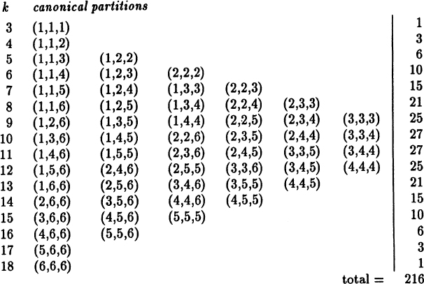
These are the increasing canonical partitions; in how many equivalent ways can each be written? If the three indices are distinct then there are evidently exactly 3! = 6 equivalent sequences in the entire sample space. If two indices are the same then the other index may be put in any of 3 places, hence there are 3 equivalent sequences in the sample space. Finally, if all three indices are the same then there is only one such sequence in the sample space. Thus we have to multiply each partition on the left by its multiplication factor (6, 3, or 1) and then sum across the line to get the total number of partitions that are in the original sample space and that also have the value k. These totals are given on the right. Dividing these sums by the total 216 we get the corresponding probabilities. When we notice the structure of the table, the symmetry of the totals above and below the middle, and check by adding all the numbers to see that we have not missed any, then we are reasonably confident that we have not made any mistakes.

The answer to the question asked of Galileo, the ratio of the probabilities of a sum of 9 or 10, is clearly 25/27 ~ 0.926. Although there are the same number of canonical partitions in these two cases, the partitions do not have the same total number of representatives in the original sample space.

At the time of Galileo there were claims that the canonical partitions are the equally likely elements of the sample space. Hence you should review the argument we gave for the product sample space of probabilities to see if it convinces you.

The reader needs to be careful! The distribution we have used is known as the Maxwell-Boltzmann distribution. If we take the canonical partitions as the equally likely elements then the distribution is known as the Bose-Einstein distribution, which assumes that it is the entries on the left hand side of Table 2.4–1 that are the equally likely events and they have no corresponding multiplicative factors. Thus the right hand column would be the sequence (1, 1, 2, 3, 4, 5, 6, 6, 6, 6, 5, 4, 3, 2, 1, 1). The total number of equally likely cases is 56.

Finally, if we consider the Pauli exclusion principle of quantum mechanics then only the canonical partitions for which the three entries are distinct can occur and these are the equally likely events. We then have the Fermi-Dirac distribution. Thus in Table 2.4–1 we must eliminate all the entries for which two of the numbers are the same. When we do this we find, beginning with the sum 6 and going to the sum 15, sequence (1, 1, 2, 3, 3, 3, 3, 2, 1, 1). The total number of cases is 20.

Only the last two distributions, the Bose-Einstein and the Fermi-Dirac, are obeyed by the particles of physics. Thus you cannot argue solely from abstract mathematical principles as to which items are to be taken as the equally likely events; we must adopt the scientific approach and look at what reality indicates. If we wish to escape the medieval scholastic way of thinking then we must make a model, compute what to expect, and then verify that our model is (or is not) closely realized in practice (except when using “loaded dice”).

Example 2.4–5    Bose-Einstein Statistics

If we put n indistinguishable balls in k cells then the number of ways we can do this is C(n; j₁, j₂, … j_k) equally likely ways, where the sum of the j_i is n. Hence any one configuration has the probability of the reciprocal of this number.

Example 2.4–6    Fermi-Dirac Statistics

Suppose we have k (indistinguishable) balls to put into n distinct boxes, (k ≤ n), and ask, “In how many ways can this be done so that at most one ball goes into any one box?”

We can select the k places from the n possible ones in exactly

$C(n,k)$

ways, and each way is equally likely. Hence the probability of any one configuration is

$1/C(n,k)$

Exercises 2.4

2.4–1 Write out the table corresponding to (2.4–2) for the Bose-Einstein statistics.

2.4–2 Write out the table corresponding to (2.4–2) for the Fermi-Dirac statistics.

2.4–3 What is the probability of no defects in n items each having a probability of a defect p?

2.4–4 Using Exercise 2.4–3 what is the probability of two or more defective pieces?

2.4–5 Show that for large n b(1; n, 1/n) ~ 1/e.

2.4–6 Similarly show that $b(2;n,1/n)~1/2e$, and $b(3;n,1/n)~1/6e=1/3!e$.

2.4–7 If p is the probability of a Bernoulli event and we make n trials show that the probability of an even number of events is [1 + (2p − 1)ⁿ]/2.

2.4–8 Corresponding to Table 2.4–1 make a table of b(k, 10,3/5).

2.4–9 If a coin is biased with probability p(H) = p then in the game of “odd man out” (see Exercise 1.7–15) what is the probability of a decision? Ans. 3pq.

2.4–10 From an R-dimensional cube of lattice points and with a side n we select a random point. Show that the probability of the point being inside the cube is ${[(n-2)/n]}^n~e^{-2}$.

2.4–11 Expand the binomials in the probabilities of 0, 1, 2, and 3 occurrences, and show that the expansions cancel out to the next term provided np < 1. Hence if np ≪ 1 the first term neglected in the expansion is close to the exact result for 4 or more events.

2.4–12 Show by exact calculation that the floppy disc estimates in Example 2.4–3 are sufficiently accurate.

2.4–13 Find the distribution of the sum of two dice following the method used for three dice for the three distributions, Maxwell-Boltzmann, Bose-Einstein, and Fermi-Dirac.

2.4–14 If a coin has probabilty p of being a head show that the probability of k tosses of the coin will have the same side is p^k + q^k. For what p is this a minimum?

2.4–15 Quality Control In a set of 106 items 10 are defective. What is the probability that a sample of 18 will aH be good? Ans. ~1/e.

2.4–16 Using the approximation exp(x) ~ (1 + 1/n)^nx and a similar one for exp(−x), discuss their product and what it indicates.

2.5    Random Variables, Mean and the Expected Value

We now introduce the idea of a random variable. We have, so far, discussed carefully the elementary events and the probabilities to assign to each. We now assign a value to the outcome of the event. For example, when we discussed the sum of the faces of three dice (Example 2.4–4) we had the value k associated with selected outcomes, namely where the sum of the three faces was equal to k. Thus we were assigning both a value 1,2, …, 6 to each of the corresponding faces of a die and also a value to the sum of the three faces. We wrote

$\mathrm{Pr}\{S=k\}$

and we now understand S to be a random variable having values running from 3 to 18 with the corresponding probabilities Pr{S = k}. S is regarded as a function over the subsets of the sample space and

$\mathrm{Pr}\{S=k\}$

is the sum of the probabilities of all outcomes which have the corresponding value k. This idea will be used extensively in the future, and if it is at first confusing this is the normal situation. The random variable idea arises because we assign values to the outcomes—the use of only names greatly restricts what we can compute.

Sometimes we want to know only a specific probability, but often we want to know the whole distribution for the random variable K which takes on the integer values k = 0,1,… ,n with probabilities P(k) = Pr{K = k} of exactly k successes in n trials (recall Table 2.4–1). In many cases, however, the actual numbers that make up the distribution are not easily assimilated by the human mind, and we need some summarizing descriptions of the distribution.

The first useful summarizing number is the mean (average)

${\displaystyle \sum _{k=0}^{n}kp(k)=0p(0)+1p(1)+2p(2)+\cdots +np(n)=\mu }$

(2.5–1)*

which is the mean value of the random variable K whose values are k = 0,1,… ,n, each with the corresponding probability p(k). This is usually labeled by the Greek lower case letter μ (mu), especially in statistics. It measures the position of the “center of the distribution.” It is the mean value of the random variable K. It is also called the average or expected value of the random variable, or of the distribution.

Example 2.5–1    The Expected (Mean) Value from the Roll of a Die

The random roll of a die gives the faces 1, 2, 3, 4, 5, 6 each with probability 1/6. If we assign the values 1, 2, 3, 4, 5, 6 to the corresponding faces then the expected (average, mean) value

$\mu =\frac{1}{6}[1+2+3+4+5+6]=\frac{1}{6}[6\times 7/2]=3.5$

which is not a possible value from any roll. The expected value is not necessarily a value that can be “expected” to turn up! It is, at the moment, only a technical definition and not necessarily what a normal human would think! You have to be a very poor statistician to believe an expected value is a value you can always expect to see.

Example 2.5–2    The Expected Value of a Coin Toss

The random toss of a coin may be given the values: head = 1 and tail = 0. Thus the expected value of a toss (p = 1/2) is

$\mu =\frac{1}{2}[1+0]=\frac{1}{2}$

However, we might have assigned the values: head = 1 and tail =—1. In this case the expected value would be

$\mu =\frac{1}{2}[1-1]=0$

Which of these two assignments of values for the faces of the coin to use depends on the particular application—the assignment of values to the outcomes of the trials depends on the use you intend to make of the result. If you are counting the number of heads in a sequence of n tosses then the first assignment is reasonable and μ = 1/2 is appropriate, but if you win one unit on a head and lose one unit on a tail then μ = 0 is more reasonable; on a single toss you expect neither a gain nor a loss.

Example 2.5–3    The Sum of Two Dice

What is the expected value of the sum of the faces of two randomly thrown dice? We start with the sample space of 6 × 6 = 36 events each with probability of 1/36, (Exercise 1.6). We are interested in the sum so we now group together all events that have the same sum of the two faces, a value running from 2 to 12. This sum S is a random variable, say S = X₁ + X₂ where the X₁ is the random variable for the first die and X₂ is the random variable for the second die. We have the following Table 2.5–1:

TABLE 2.5–1

Table of S = X₁ + X₂

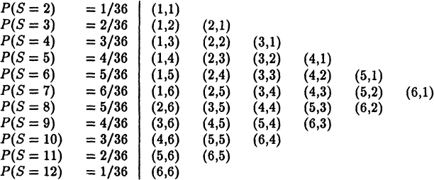
The table on the right lists the 36 equally likely entries in the sample space in a convenient order. The derived random variable S does not have a uniform distribution though it comes from a uniform distribution via grouping various terms having the same value for the random variable S (the sum). The expected value of the distribution of S is (for the standard value assignment to the outcomes)

$\mu =[2\times 1+3\times 3+4\times 3+5\times 4+6\times 5+7\times 6+8\times 5+9\times 4+10\times 3+11\times 2+12\times 1]/36=252/36=7$

But this is just the sum of the expected values from each of the two independently thrown dice! This is not a coincidence as we will see below. Thus further investigation of the expected value of a distribution (with a given value assignment) is worth some effort.

We see that the mean (average) or expected value is merely the sum of the values assigned to the outcomes of each trial when each outcome is weighted by the probability of its occurrence. This weighting of the values of the outcomes of the occurrences by their corresponding probabilities happens frequently and we need, therefore, a notation and some simple results to relieve us of rethinking the details every time we compute a mean. Given a random variable X whose outcomes have probabilities p(i), and have the values x_i, (i = 1,2,…, n), then the expected value of the random variable X is defined to be (E is for expectation)

$E\left\{X\right\}={\displaystyle \sum _{i=1}^n{x}_{i}p(i)}$

(2.5–2)*

This is the average computed over the sample space, each outcome value x_i is weighted by its probability p(i).

The expected value operator E{.} is a linear operator whose properties are worth investigating. We first examine the expected value of the product of two random independent variables X and Y, and then examine the sum.

For the product XY, of the two random, independent variables X and Y the probability of the pair of outcomes x_i and yj will by definition (2.5–2) be

$E\left\{XY\right\}={\displaystyle \sum _{k}kp\{XY=k\}}$

(2.5–3)

How do we get the p{XY = k}? By definition (2.5–2) we must first sum all the px(i)py(j) in the sample space for which x_iy_j = k, where the subscripts on the probabilities indicate the corresponding variable. Hence we have

$E\left\{XY\right\}={\displaystyle \sum _{k}k}{\displaystyle \sum _{x_i{y}_j=k}pX(i)pY(j)}$

This formula is not easy to use so we seek an alternate approach to compute E{XY}. We go back to (2.5–2). The product x_iy_j arises with probability Px(i)py(j), hence

$\begin{array}{ll}E\left\{XY\right\}\hfill & ={\displaystyle \sum _{\begin{array}{c}\text{sample}\\ \text{space}\end{array}}{x}_i{y}_{j}pX(i)pY(j)}\hfill \\ \hfill & ={\displaystyle \sum _i{\displaystyle \sum _j{x}_i{y}_{j}pX(i)pY(j)}}\hfill \end{array}$

(2.5–4)

We need to convince ourselves that these two different expressions (2.5–3) and (2.5–4) for E{X} are the same. To see this take any point in the product sample space (x_i,y_j) and follow it through each computation; you will see that it enters into the result exactly once and only once either way, each time with weight pX(i)pY(j). Hence the two formulas represent alternate ways of finding the expected value.

This proof of the equivalence is simple for a finite discrete sample space, but when we later face continuous sample spaces it brings up two separate ideas. First, the integral (corresponding to the finite summation) over the whole sample space is the iterated integral (in either order) as in the calculus. Second, a change of variables (in this case from rectangluar to what will be an integration along a hyperbolic coordinate and then all the hyperbolas are integrated to cover the whole sample space) to new coordinates will involve the corresponding Jacobian of the transformation.

We now return to the problem at hand. Taking it in the second form, (2.5–4), we have the expected value of the product of the independent variables

$E\left\{XY\right\}={\displaystyle \sum _{i,j}{x}_i{y}_{j}pX(i)pY(j)}$

If we fix in our minds one of the variables, say x_i, and sum over the y variable we will find that for each value x_i we will get the expected value of Y, namely E{Y}. This will factor out of each term in the variable x_i, hence out of the sum. What is left is the expected value of X. Thus we have the result that for independent random variables

$\begin{array}{ll}E\left\{XY\right\}\hfill & ={\displaystyle \sum _i{x}_{i}pX(i)}{\displaystyle \sum _j{y}_{j}pY(j)}\hfill \\ \hfill & =E\left\{X\right\}E\left\{Y\right\}\hfill \end{array}$

(2.5–5)

A rather simple way to see this important result is to actually write out the product space of the random independent variables X and Y in a rectangular array.

$\left|\begin{array}{cccc}{x}_1{y}_{1}pX(1)pY(1)& x_1{y}_{2}pX(1)pY(2)& \cdots & x_1{y}_{n}pX(1)pY(n)\\ x_2{y}_{1}pX(2)pY(1)& x_2{y}_{2}pX(2)pY(2)& \cdots & x_2{y}_{n}pX(2)pY(n)\\ \cdots & \cdots & & \cdots \\ x_n{y}_{1}pX(n)pY(1)& x_n{y}_{2}pX(n)pY(2)& \cdots & x_n{y}_{n}pX(n)pY(n)\end{array}\right|$

Now consider summing by the rows; for the ith row the x_ipx(i) value is fixed and you get for every row the same value E{Y}. Now sum what is left after factoring out the E{Y} and you get E{X}. Alternately, you can sum by the columns first to get E{X} and then sum the rest to get the E{Y}. In both cases you get the product of the expectations.

Next we consider the sum of any two random variables X and Y, independent or not. We have

$E\{X+Y\}={\displaystyle \sum _i^j(x_i+y_j)p(i,j)}$

where p(i,j) is the probability of the pair x_i, y_j occurring. When you think about the two following equations you see why they are true:

$\begin{array}{l}{\displaystyle \sum _{j}p(i,j)=pX(i)}\\ {\displaystyle \sum _{i}p(i,j)=pY(j)}\end{array}$

(2.5–6)

We have, therefore, on breaking up the sum into two sums and then interchanging the order of summation in the second sum,

$\begin{array}{l}\begin{array}{ll}E\{X+Y\}\hfill & ={\displaystyle \sum _i^j(x_i+y_j)p(i,j)}\hfill \\ \hfill & ={\displaystyle \sum _i{x}_i}{\displaystyle \sum _{j}p(i,j)}+{\displaystyle \sum _j{y}_j}{\displaystyle \sum _{i}p(i,j)}\hfill \\ \hfill & ={\displaystyle \sum _i{x}_{i}pX(i)}+{\displaystyle \sum _j{y}_{j}pY(j)}\hfill \end{array}\\ =E\left\{X\right\}+E\left\{Y\right\}\end{array}$

This should be clearly understood because it is fundamental in many situations. We have the result that the expected value of the sum of two random variables, independent or not, is the sum of their expected values,

$E\{X+Y\}=E\left\{X\right\}+E\left\{Y\right\}$

(2.5–7)

It is an easy extension to see that E{.} is a linear operator, that is

$E\{aX+bY\}=aE\left\{X\right\}+bE\left\{Y\right\}$

(2.5–8)*

We have only to follow through the above argument with the constants a and b and notice how they factor out of each sum. This result shows why the expected value of the sum of the values of the two dice is the sum of their expected values.

The fact that the expectation of a sum of random variables is the sum of the expectations no matter how the two variables are related explains why E{.} is such a useful linear operator.

This method of summing over one of the variables and then over the other, and finding that the expected value factors out of the other sum and that then the other sum is exactly 1, is fundamental to much of the theory and should be mastered. If you do not see it clearly then look again at the product space (the rectangular array) and examine what happens as you sum (x_i + y_j) by rows and then by columns.

Once we notice that the sum of two random variables is itself a random variable, then we can recursively apply the above formula and obtain result that for any finite sum of random variables X_i with constants c_i

$E\left\{{\displaystyle \sum c_i{X}_i}\right\}={\displaystyle \sum c_{i}E\left\{X_i\right\}}$

(2.5–9)*

For products of independent random variables we have correspondingly

$E\left\{{\displaystyle \prod _i[X_i]}\right\}={\displaystyle \prod _i[E\{X_i\}]}$

(2.5–10)*

these generalize equations (2.5–7) and (2.5–5).

Other measures of a distribution besides the expected value are often used by statisticians. One is the median which is the middle value when the x_i are ranked in order (the average of the middle two when there are an even number of values). Another measure is the mode which is the most frequent (most fashionable) value. The mode makes sense only when the distribution has a single, well defined, peak. The mid range (x_max – x_min)/2 is occasionally used.

Example 2.5–4    Gambling on an Unknown Bias

You have a sequence of repeated, independent trials of unknown probability p, say betting on a biased coin. One strategy for betting is to bet on the face of the most recent outcome thus making your bets have the same frequency as the out comes of the trials. Your expected gain per trial is

$\text{gain}-\text{loss}=pp+qq-\{pq+qp\}={(p-q)}^2$

If you have the additional information that the bias is such that p > 1/2 then an alternate strategy is to bet always on the event. Now your gain per toss is

$(p-q)$

Thus knowing only the side which the bias favors, you have a significant advantage (except for p = 1/2 and p = 1) as the following table shows.

prob. p	gain 1	gain 2
.5	.00	.0
.6	.04	.2
.7	.09	.4
.8	.16	.6
.9	.64	.8
1.0	1.00	1.0

Mathematical aside: Sums of Powers of the Integers

We often need some small mathematical details that are not easily recalled by the student. In particular we will often need the sums of the consecutive integers raised to low powers; we will need the formulas

$\begin{array}{l}{\displaystyle \sum _{k=1}^{n}k=n(n+1)/2}\\ {\displaystyle \sum _{k=1}^n{k}^2=n(n+1)(2n+1)/6}\\ {\displaystyle \sum _{k=1}^n{k}^3={[n(n+1)/2]}^2}\end{array}$

These are all easy to prove by the use of mathematical induction. For example, for the sum of the cubes of successive integers we need to show: (1) for the basis of the induction, using n = 1, we get the same number on both sides, and (2) for the induction step from n − 1 to n we have an equality, namely

$\begin{array}{l}\text{old sum}+\text{next term}=\text{new sum}\\ \begin{array}{ll}{[n(n-1)/2]}^2+n^3\hfill & =n^2[(n^2-2n+1)/4+n]\hfill \\ \hfill & =n^2[{(n+1)}^2/4]={[n(n+1)/2]}^2=\text{ new sum}\hfill \end{array}\end{array}$

Exercises 2.5

2.5–1 Cannon balls are piled as a pyramid with a square base. If the side of the square is n, then how many balls in the pile?

2.5–2 Triangular numbers are defined as f(n) = n(n − 1)/2. Find the sum of the first k triangular numbers.

2.5–3 What is the expected value for a deck of cards numbered (values) 1, 2,…, 52?

2.5–4 What is the expected value of the sum of four dice?

2.5–5 What is the expected value of the sum of n coins? Ans. n/2 or 0.

2.5–6 What is the expected value of the sum of n dice?

2.5–7 One and only one key on a key chain of n keys fits the lock. Compare finding the key by systematic or random methods.

2.5–8 A disc track is selected from a set numbered 1, 2, …, n. Call this X. You now select Y from 1 ≤ y ≤ X. Show that E{Y) = (n + 3)/4.

2.5–9 If p(k) = k/10, (0 ≤ k ≤ 4) find E(K).

2.5–10 If p(k) = qp^k(k = 0, 1, …) find E(K).

2.5–11 Find the product of the values on the two faces of a pair of independently thrown dice. Ans. 49/4.

2.5–12 What is the expected value of the product of three independently thrown dice?

2.6    The Variance

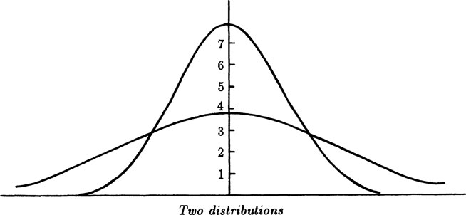
The mean gives the location of the “center” of a distribution, but a little experience with distributions soon shows that some distributions are spread out and some are narrow; see Figure 2.6–1. The amount of the spread is often important so we need a measure of the “spread” of a distribution. The most useful one from the point of view of mathematics (meaning it can be handled easily) is the sum of the squares of the deviations from the mean, μ, each square of course multiplied by its probability p(i),

FIGURE 2.6–1

$\text{Variance}\left\{X\right\}=V\left\{X\right\}={\displaystyle \sum _i{(x_i-\mu )}^{2}p(i)={\sigma }^2}$

(2.6–1)*

The standard notation is σ², where σ is often used as a measure for the spread of the distribution of the random variable X. A large variance means that the distribution is broad, and a small variance means that the all distribution is near the mean. Indeed, a zero variance means that the distribution is all at one point, the mean, μ. Note, like the mean, the variance is computed over the whole sample space.

It is immediately evident that the variance is independent of any shift in the coordinate axis, since it depends only on the difference of coordinates and not on the coordinates themselves. This is important because it allows us, many times, to simplify various derivations by assuming that the mean is zero.

We need the facts that (c is a constant)

$\begin{array}{cc}V\left\{c\right\}=0& V\left\{cX\right\}=c^{2}V\left\{X\right\}\end{array}$

(2.6–2)*

The first follows because the variance is measured about the mean (which is c), and the second because by the definition a multiplying factor c will also multiply the mean by c, and hence c² comes out of the square of the differences.

For theoretical work we often convert the formula for the variance to a more useful form. We simply expand the square term in (2.6–1) and note how the mean arises, (E{X} = μ)

$V\left\{X\right\}=E\left\{X^2\right\}-2\mu E\left\{X\right\}+{\mu }^2=E\left\{X^2\right\}-E^2\left\{X\right\}$

(2.6–3)*

Next, we prove that for a sum of independent random variables X_i we have (V{.} is a linear operator)

$V\left\{{\displaystyle \sum X_i}\right\}={\displaystyle \sum V\left\{X_i\right\}}$

(2.6–4)*

The proof is easy. For convenience we assume that the mean of each random variable X_i is 0, E{X_i) = 0. Then we have, (using different summation indices to keep things straight)

$\begin{array}{ll}E\{{\displaystyle \sum X_i^2\}}\hfill & =E\left\{{\displaystyle \sum X_i}{\displaystyle \sum X_j}\right\}\hfill \\ \hfill & =E\left\{{\displaystyle \sum _{i,j}{X}_i{X}_j}\right\}\hfill \\ \hfill & =E\left\{{\displaystyle \sum _i{X}_i^2}\right\}+E\left\{{\displaystyle \sum _{i\ne j}{X}_i{X}_j}\right\}\hfill \end{array}$

where the squared terms are in the first summation and the cross products are in the second (each there twice). But for independent random variables from (2.5–5) E{X_iX_j} = E{X_i}E{X_j) = 0 × 0 = 0 (since we assumed the means were 0). Hence the last sum is zero. Therefore, for independent random variables the variances simply add, a very useful property:

$V\left\{{\displaystyle \sum X_i}\right\}={\displaystyle \sum V\left\{X_i\right\}}$

(2.6–5)*

Thus the variance of the sum of n samples of the same random variable has the variance nσ².

The mean and variance we have just computed are probability weighted averages of the values over the whole sample space. Often for just n random sample values from the distribution we want to know expected value and the variance of their average. Thus we need to study the average of the n samples. We do not want to actual handle the specific samples, so we write their corresponding random variables X_i, and examine the random variable

$S(n)=X_1+X_2+\cdots +X_n$

We want to study the average so we use

$S(n)/n=[X_1+X_2+\cdots +X_n]/n$

For the expected value of the average S(n)/n we have

$\begin{array}{ll}E\{S(n)/n\}\hfill & =[E\{X_1\}+\cdots +E\{X_n\}]/n\hfill \\ \hfill & =[\mu +\mu +\mu +\cdots +\mu ]=\mu \hfill \end{array}$

Thus the expected value of the average of n samples is exactly the expected value of the original random variable X—it is an unbiased estimate since it is neither too high nor too low.

For the variance of the average of n independent samples we assume the mean is 0 and have

$\begin{array}{ll}V\{S(n)/n\}\hfill & =[V\{X_1\}+\cdots +V\{X_n\}]/n^2\hfill \\ \hfill & ={\sigma }^2/n\hfill \end{array}$

Thus the variance of the average of n samples of a random variable decreases like 1/n. The corresponding measure of the spread of the distribution (compare 2.4–6) of the average of n samples is

$\sigma /\sqrt{n}$

This means that if we want to decrease the spread of a distribution of the average of n samples by a factor of 10 we will need to take 100 times as many samples.

How robust are these measures to small changes in the probabilities p(i)? If the p(i) are not exactly what we supposed they were but have errors e(i), then the true values are

$p(i)+e(i)$

where we have, of course, ${\displaystyle \sum e(i)=0}$. We should have computed

$E{\left\{X\right\}}^{*}={\displaystyle \sum x_i[(p(i)+e(i)]=E\{X\}}+{\displaystyle \sum x_{i}e(i)}$

and we lost the last sum. For convenience we write

$\begin{array}{ccc}E{\left\{X\right\}}^{*}={\mu }^{*}& \text{and}& E\left\{X\right\}=\mu \end{array}$

and we have

$\begin{array}{ccc}{\mu }^{*}=\mu +{\displaystyle \sum x_{i}e(i)=\mu +A}& \text{or}& {\mu }^{*}-\mu =A\end{array}$

where we have set $A={\displaystyle {\sum }_i{x}_{i}e(i)}$ and A is therefore the shift in the mean.

The variance is more complex. We should have computed

$V^{*}={\displaystyle \sum {(x_i-{\mu }^{*})}^2(p(i)+e(i))}$

Instead we computed

$V={\displaystyle \sum {(x_i-\mu )}^{2}p(i)}$

To get V* in terms of simpler expressions, especially V, we write things as

$V^{*}={\displaystyle \sum {(x_i-\mu -A)}^{2}p(i)}+{\displaystyle \sum {(x_i-\mu -A)}^{2}e(i)}$

Expand the binomials and get term by term

$\begin{array}{l}{V}^{*}=V-2A{\displaystyle \sum (x_i-\mu )p(i)+A^2}\\ +{\displaystyle \sum {(x_i-\mu )}^{2}e(i)-2A}{\displaystyle \sum (x_i-\mu )e(i)+A^2}{\displaystyle \sum e(i)}\end{array}$

The second and sixth terms and part of the fourth and fifth drop out and if we set ${\displaystyle \sum x_i^{2}e(i)}=B$ then we have

$\begin{array}{ll}{V}^{*}\hfill & =V+A^2+B-2\mu A-2A^2\hfill \\ \hfill & =V+B-A(2\mu +A)\hfill \end{array}$

Example 2.6–1    The Variance of a Die

The roll X of a die has, (from Example 2.5–1), E{X} = 7/2. The variance is the values measured from the mean, then squared, and finally summed over all the values weighted by their probabilities p(i). We get, for the standard assignment of values for the faces of the die, the differences from the mean

$\begin{array}{llllll}-5/2,\hfill & -3/2,\hfill & -1/2,\hfill & 1/2,\hfill & 3/2,\hfill & 5/2\hfill \end{array}$

to be squared, multiplied each by p(i)= 1/6, and added. As a result we get

$(1/6)[25+9+1+1+9+25]/4=70/24=35/12$

Instead we can compute the squares of 1, 2, 3, 4, 5, 6, add, and then multiply the sum by the probability 1/6, to get E{X²} = 91/6. According to (2.6–3) we then subtract the square of the mean

$91/6-{(7/2)}^2=91/6-49/4=(182-147)/12=35/12$

which is, of course, the same number.

Notice that the formula (2.6–3) may (as in this example) give a difference of large numbers and hence be sensitive to roundoff errors, especially when the mean is large with respect to the variance.

Example 2.6–2    Variance of M Equally Likely Outcomes

This is a generalization of Example 2.6–1. We have the x_i = i, (i = 1,…, M), p(i) = 1/M, and the sums

$\begin{array}{ll}{\displaystyle \sum 1}\hfill & =M\hfill \\ E\left\{X\right\}\hfill & =(1/M){\displaystyle \sum x_i=(1/M)M(M+1)/2=(M+1)/2}\hfill \\ E\left\{X^2\right\}\hfill & =(1/M){\displaystyle \sum x_i^2=(1/M)M(M+1)(2M+1)/6}\hfill \\ \hfill & =(M+1)(2M+1)/6\hfill \end{array}$

hence the variance is

$\begin{array}{ll}V\hfill & =[(M+1)][(2M+1)/6-(M+1)/4]\hfill \\ \hfill & =(M+1)[4M+2-3M-3]/12\hfill \\ \hfill & =(M+1)(M-1)/12=(M^2-1)/12\hfill \end{array}$

For M = 6 this gives 35/12 as before, Example 2.6–1.

Example 2.6–3    The Variance of the Sum of n Dice

If we assume, as we should since nothing else is said, that the outcomes of the roll of n individual dice are independent and uniformly likely, then by (2.6–5) we merely take the variance of a single die and multiply by n

$(35/12)n$

to get the variance of the sum of n dice.

There is a tendency to believe that the square root of the variance gives a good measure of the expected deviation from the mean. But remember that we “averaged” the squares of the deviations from the mean. In the sum of the squares the big deviations tend to dominate the sum (since the square of a large number is very large and the square of a small number is small, hence only the large numbers influence the total very much). Thus it should be clear that if the deviations from the mean vary a lot then the square root of the variance is not a good measure of the expected deviation, which should be given by a formula like (although μ should probably be computed by a different formula, say the median)

$E|X-\mu |={\displaystyle \sum _i|x_i-\mu |p(i)}$

This is the average of the absolute differences from the mean (or maybe the median). It is not used much because it has difficult mathematical properties (but often good statistical properties!).

Consider the equally likely data (p(i) = 1/10)

$x_1=6,x_2=x_3=\cdots =x_{10}=1$

The mean is (6 + 9)/10 = 1.5, hence the variance is

$\text{Var}=(1/10)[{(4.5)}^2+9{(0.5)}^2]=(20.25+2.25)/10=2.25$

Hence the root mean square (the square root of the mean of the quares) is 1.5. On the other hand the mean deviation from 1.5 (the mean) is

$(1/10){\displaystyle \sum |x_i-1.5|=(1/10)[4.5+9(1/2)]=9/10=0.9}$

The difference in the two answers is due mainly to the “outlier” x₁ = 6. When is 1.5 a better measure of the deviation from a reasonable estimate of the center of the distribution than is 0.9 given nine values at 1 and one value at 6? It all depends on the use to be made of the result! Had we used the median, which is 1, and found the mean deviation from it we would, in this case, have found the result 1/2.

The sequence E{1} = 1, E{X}, and E{X²} suggests that the general kth moment should be defined by

$E\left\{X^k\right\}={\displaystyle \sum _i{x}_i^{k}p(i)}$

(2.6–5)*

If we want the k^th moment about the mean (the k^th central moment) then we have

$E\left\{{(X-\mu )}^k\right\}={\displaystyle \sum _i{(x_i-\mu )}^{k}p(i)}$

(2.6–6)*

For most purposes all the moments determine, theoretically, the distribution, and play a significant role in both probability and statistics. In practice only the lower moments are used—because as noted above the larger terms dominate in the sum of the squares and this is even more true for higher powers. The third moment about the mean is called “skewness” and the fourth is called “kurtosis” (elongation, flatness); the higher ones, have not even been named! Similarly,

$E\{f(n)\}={\displaystyle \sum _{i}f(i)p(i)}$

(2.6–7)*

for any reasonable function f(n).

Exercises 2.6

2.6–1 For the formula (2.6–5) find for k = 3, 4, and 5 the central moments in terms of the moments about the origin.

2.6–2 Carry out the derivation of the formula for the variance when the mean is μ.

2.6–3 Find the variance of n trials from a sample space of M equally likely events.

2.6–4 Conjecture that the sum of the fourth powers of the integers is a polynomial in n of degree five. Impose the induction hypothesis (and initial sum) and deduce the corresponding coefficients of the fifth degree polynomial.

2.6–5 Find the mean and variance of a Bernoulli distribution.

2.6–6 Find the third and fourth moments of a Bernoulli distribution.

2.6–7 Find the mean and variance of the distribution {qpⁿ} (n = 0,1,…). Ans. p and p/q².

2.6–8 For the distribution p(k) = k/10 (k = 0, …,4) find the mean and variance.

2.7    The Generating Function

Given a probability distribution p(k) (for integer values k) we can write it as a single expression by means of the generating function which is a polynomial in the variable t whose coefficients are the values p(k)

$G(t)={\displaystyle \sum _{k}p(k)t^k=E\left\{t^k\right\}}$

(2.7–1)*

For example, for a die with six faces each of probability 1/6, we have the generating function

$\begin{array}{ll}G(t)\hfill & =(t+t^2+t^3+t^4+t^5+t^6)/6\hfill \\ \hfill & =t(1-t^6)/6(1-t)\hfill \end{array}$

We have seen the generating function before, but in the form used for counting or enumerating. For example, for the binomial coefficients we had (2.3–2) the generating function

$G(t)={(1+t)}^n={\displaystyle \sum _{k=0}^{n}C(n,k)t^k}$

This suggests immediately that for the binomial (Bernoulli) probability distribution (2.4–2)

$b(k;n,p)=C(n,k)p^k{q}^{n-k}$

we will have the generating function (see 2.4–5)

$G(t)={\displaystyle \sum _{k=0}^n\{C(n,k)p^k{q}^{n-k}\}{t}^k={(q+pt)}^n}$

(2.7–2)

The generating function representation of a probability distribution is very useful in many situations; the whole probability distribution is contained in a single expression. It should be evident from (2.7–1) that

$G(1)={\displaystyle \sum _{k}p(k)=1}$

If we differentiate the generating function with respect to t we get

$G^{\prime }(t)={\displaystyle \sum _{k}kp(k)t^{k-1}}$

and hence

$G^{\prime }(1)=\mu =E\left\{X\right\}$

(2.7–3)*

If we multiply G’(t) by t and then differentiate again we will get

$[t{G}^{\prime }(t){]}^{\prime }=t{G}^{″}(t)+G^{\prime }(t)={\displaystyle \sum _k{k}^{2}p(k)t^{k-1}}$

and hence we have (set t = 1 again)

$E\left\{X^2\right\}=G^{″}(1)+G^{\prime }(1)$

Therefore, the second moment about the mean is simply (2.6–3)

$V\left\{X\right\}=G^{″}(1)+G^{\prime }(1)-{[G^{\prime }(1)]}^2={\sigma }^2$

(2.7–4)*

We see that from the generating function alone we can get by formal differentiation both the mean and variance of a distribution (as well as higher moments if we wish). Thus the generating function is a fundamental tool in handling distributions and solving probability problems.

Example 2.7–1    The Mean and Variance of the Binomial Distribution

From (2.7–2) the generating function for the binomial distribution and its first two derivatives are

$\begin{array}{l}G(t)={(q+pt)}^n\\ G^{\prime }(t)=np{(q+pt)}^{n-1}\\ G^{″}(t)=n(n-1)p^2{(q+pt)}^{n-2}\end{array}$

We now set t = 1 and get the values (remember that p + q = 1)

$\begin{array}{l}G(1)=1\\ G^{\prime }(1)=\mu =np\\ G^{″}(1)=n(n-1)p^2\end{array}$

hence we have for the binomial distribution (use (2.7–4))

$\text{mean}=\mu =np$

(2.7–5)*

$\begin{array}{ll}\text{variance}\hfill & ={\sigma }^2=n(n-1)p^2+(np)-{(np)}^2\hfill \\ \hfill & =np(1-p)=npq\hfill \end{array}$

(2.7–6)*

The generating function allows us to do much more. If we ask how the sum of the faces of two dice can arise we see that it is the product of the generating function with itself

$\begin{array}{ll}G(t)G(t)\hfill & =(t+t^2+\cdots +t^6)(t+t^2+\cdots +t^6)\hfill \\ \hfill & =t^2+2t^3+3t^4+\cdots +t^{12}\hfill \end{array}$

The coefficient of any power of t, say the k^th power, is the number of ways that the sums of the original exponents can produce that k. The number of ways this can happen is exactly the coefficient of t^k. The coefficient counts the number of ways the sum can arise. Thus we have the result that the generating function for the sum of the faces of two dice is simply the square of the generating function for a single die.

This is a general result. Since the exponent of t is the same as the value assigned to the outcome of the trial, the power series product of two generating functions (where the exponents are automatically arranged for us when we arrange things in powers of t) has for each power of t a coefficient that counts how often that sum can occur. In general, if

$\begin{array}{l}G(t)={\displaystyle \sum _i{a}_i{t}^i}\\ H(t)={\displaystyle \sum _j{b}_j{t}^j}\end{array}$

(3.7–8)

where the summations begin with index 0 to allow for a possible constant term), then for the product we have

$G(t)H(t)={\displaystyle \sum _k{c}_k{t}^k}$

(3.7–9)*

where

$c_k={\displaystyle \sum _{i+j=k}{a}_i{b}_j}={\displaystyle \sum _{i=0}^k{a}_i{b}_{k-i}}$

(3.7–10)*

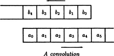
This sequence {c^k} is called the convolution of the sequence {a_i} with the sequence {b_j}.

The concept of a convolution is very useful, so we will linger over it a bit more to improve your understanding of it. We can easily picture a convolution of two sequences, one belonging to G(t) and the other to H(t). We imagine one written from left to right on a strip, beginning with the zeroth term, and the other sequence written in the reverse direction (right to left) on the other strip, as shown in Figure 2.7–1. The second is placed below the first and is also displaced so that the k^th term of one is opposite the zeroth term of the other. The sum of the products of the overlapping terms is exactly the convolution of the two corresponding sequences. In more detail we start with the zeroth terms opposite each other, compute to get the value for $c_0=a_0{b}_0$; shift one strip one unit, compute to get the value for $c_1=a_0{b}_1+a_1{b}_0$; shift, compute $c_2=a_0{b}_2+a_1{b}_1+a_2{b}_0$; … until we get all the coefficients c_k we want. The convolution of G(t) with H(t) is the same as the convolution of H(t) with G(t) as can be seen from the figure or else from the formula (3.7–10) by replacing the dummy summation index i by k – i. Hence the convolution operation is commutative {it must be since G(t)H(t) = H(t)G(t)}.

FIGURE 2.7–1

Example 2.7–2    The Binomial Distribution Again

With the idea of a convolution in mind we start with the simple observation that a single binomial choice with probabilities p and q has the generating function

$G(t)=(q+pt)$

hence the sum of n independent binomial choices will have this same generating function raised to the nth power, (2.7–2),

$G^n(t)={(q+pt)}^n$

as we should. From the expression for G(t) = (q + pt) we see that G’(1) = p and G”(1) = 0, hence using (2.5–6) and (2.6–3) we have for the binomial distribution of order n

$\begin{array}{l}\mu =np\\ \text{Var}=n(0+p-p^2)=np(1-p)=npq\end{array}$

as before, Example 2.7–1.

Example 2.7–3    The Distribution of the sum of Three Dice

At the start of this Section we gave the generating function of the face values of the roll of a single die,

$G(t)=t(1-t^6)/6(1-t)$

To get the generating function for the roll of 3 dice we merely cube this. It is not going to be easy to get the coefficients of this generating function by a power series expansion, (but see Example 2.4–4). Instead we can use the idea of a convolution and observe that the roll of 2 dice is the convolution of the sequence with itself (neglecting the factor 1/6), where the “|” is at the beginning of the sequence (just before the 0^th term) for the first die

$|0,1,1,1,1,1,1,0,0,0\dots$

We have supplied 0 coefficients as needed. Convolving this with itself (remember to reverse the order of the coefficients on the second strip) we see that we get, neglecting the factor 36 for the moment and merely counting the number of times,

$|0,0,1,2,3,4,5,6,5,4,3,2,1,0,0,\dots$

To get the result for three dice we convolve this with the original sequence and get,

$|0,0,0,1,3,6,10,15,21,25,27,27,25,21,15,10,\dots$

as we did in Table 2.4–1. To get the probabilities we divide by 6³ = 216. A comparison of the details of the two methods of computing shows that we are making progress when we introduce the more advanced ideas of generating functions and convolution—they help make actual computation easy as well as making the thinking a lot easier.

Two things should be noted about our definition of a generating function in terms of a probability distribution. In the first place, given any sequence of numbers a_i we can define a generating function

$A(t)={\displaystyle \sum _k{a}_k{t}^k}$

The derivatives at the value t = 1 are

$\begin{array}{l}{A}^{\prime }(1)={\displaystyle \sum _{k}k{a}_k}\\ A^{″}(1)={\displaystyle \sum _{k}k(k-1)a_k}\end{array}$

There is an alternate form of a generating function that should perhaps be mentioned. The exponential generating function is defined by

$M(t)={\displaystyle \sum _k{a}_k{t}^k/k!}$

For some purposes the M(t) is useful, but the simple formulas for the mean and variance require modification.

Exercises 2.7

2.7–1 Find the generating function, mean and variance for four dice.

2.7–2 Same for two dice with one biased.

2.7–3 Same with both dice biased different amounts.

2.7–4 Apply the convolution theorem to the Bernoulli distribution and deduce various identities among the b(k;n,p).

2.7–5 Apply the generating function approach to the toss of coins. Show that for n coins you get the correct mean and variance.

2.7–6 If the generating function G(t) is the k^th power of another generating function F(t) find the first and second derivatives of G(i).

2.7–7 You draw one spade and one heart. What is the distribution of the sum of the faces using values 1, 2, …, 13 if you draw one card from each of these suits?

2.7–8 Find the distribution of a biased die rolled twice.

2.7–9 A distribution has p₀, p₁ and p₂ (with of course their sum being 1). Find the distribution of the sum of two and of three trials. Ans. For two trials, $p_0^2,2p_0{p}_1,2p_0{p}_2+p_1{p}_2^2$.

2.7–10 For the distribution {qpⁿ} find the distribution of the sum of two and of three events happening.

2.8    The Weak Law of Large Numbers

We now examine one of the most important results in the simple theory of probability, the weak Jaw of large numbers. It answers the question, “What is the expected value for the average of n independent samples of the same random variable X?” This law connects our postulated idea of probability, which is based on symmetry, with our intuitive feeling that the average approaches, in some sense, the expected value—that the formally defined expected value E{X} is actually the “expected value” from many trials. It is called the “weak law” because there is a stronger form of it which uses the limit as the number of samples approaches infinity.

Before proving this important result we need a result called the Chebyshev inequality. Given a random variable X whose values, positive or negative, are the x_i with corresponding probabilities p(i), we form the sum

$E\left\{X^2\right\}={\displaystyle \sum _i{x}_i^{2}p(i)}$

From this sum we exclude those values which are within a distance ∊(Greek lower case epsilon) of the origin. Hence we have the inequality

$E\left\{X^2\right\}\ge {\displaystyle \sum _{\left|x_i\right|\ge \in }{x}_i^{2}p(i)}$

We next strengthen the inequality by reducing all the $x_i^2$ to the smallest value they can have, namely ∊². We have

$E\left\{X^2\right\}\ge {\in }^2{\displaystyle \sum _{\left|x\right|\ge \in }p(i)}$

and on writing Pr{.} as the probability of the condition in the {.} occurring

$E\left\{X^2\right\}\ge {\in }^2\mathrm{Pr}\left\{\right|x_i|\ge \in \}$

This can be rearranged in the form

$\mathrm{Pr}\left\{\right|x_i|\ge \in \}\le E\left\{X^2\right\}/{\in }^2$

(2.8–1)*

which is known as the Chebyshev inequality.

There is another form of the Chebyshev inequality that is often more useful for thinking; this measures the deviation in terms of the quantity σ. We merely replace ∊ by σ∊. This gives us, corresponding to (2.8–1)

$\mathrm{Pr}\left\{\right|x_i|\ge \sigma \in \}\le E(X^2\}/{(\sigma \in )}^2$

(2.8–2)*

If, as we have assumed, the mean is zero then we have

$\mathrm{Pr}\left\{\right|x_i|\ge \sigma \in \}\le 1/{\in }^2$

In order to understand this important result we analyse the extreme of how the equality might arise. First, we dropped all the terms for which |x_i| < ∊. Second, we replaced all larger x_i by their minimum ∊. There might have been no terms dropped in the first step, and all the terms might have been of the minimum size in the second, so no reduction occurred and the equality held; all the values were piled up at the distance ∊ from the origin, and there were no others, but this is unlikely! In this sense the Chebyshev inequality cannot be strengthened—but other forms can be found. We could, for example, use any nonnegative function in place of $x_i^2$ if we wish to get other inequalities.

We now turn to a closer study of the average of n independent samples of a random variable X having values x_i. Since we do not want to talk about the individual sample values we will again treat the n samples as n random variables $X_i,(i=1,2,\dots ,n)$. The average is defined to be

$S(n)/n$

where

$S(n)=[X_1+X_2+\cdots +X_n]$

(2.8–3)

In the previous Section 2.7 we studied the mean and variance of S(n)/n when we averaged over the whole sample space and found their corresponding values μ and σ²/n.

Since E{.} is a linear operator, to get the expected value of the sample average S(n)/n we average over the whole sample space and get the individual E{X}. We then apply the Chebyshev inequality (2.8–1) to the difference between S(n)/n and its expected value μ,

$\begin{array}{ll}\mathrm{Pr}\left\{\right|S(n)/n-\mu |\hfill & \ge \in \}\le V\{S(n)/n\}/{\in }^{2}n\hfill \\ \hfill & \le (1/n^2)V\{S(n)\}/{\in }^2\hfill \\ \hfill & \le V\left\{X\right\}/{\in }^{2}n\hfill \end{array}$

(2.8–5)*

This is the desired result; the probability that the average of n independent samples of a random variable X differs from its expected value μ by more than a given constant ∊ is controlled by the number on the right. We see that for a random variable X by picking n large enough we can probably have the average of n samples close to the expected value μ of the random variable X.

There is a complement form (since the total probability must be 1), and using kσ in place of ∊, we get

$\mathrm{Pr}\left\{\right|S/n-a\left|\right\}<k\sigma \}>1-V\{X\}/{(k\sigma )}^{2}n$

(2.8–6)*

that is often useful. One form says that it is unlikely that the sample average will be far out, the other that it is probable it will be close.

The results may seem to apply only to binary choices, but consider a die. The application with p = 1/6 applies to each face in turn, (with probability 5/6 for all the other faces), hence each face will have the ratio of 1 to 6 for success to total trials. Similarly, any multiple choice scheme can be broken down to a sequence of two way choices, one choice for one given outcome and the other for all the rest combined, and then applied to each outcome in turn.

In this derivation we found an upper bound on the probability—but the earlier result for the binomial distribution 2.4–6 shows that the deviation of the average from the mean is actually

$1/2\sqrt{n}$

and suggests that this is the probable behavior in the general case; we can reasonably expect the square root of the variance to be a measure of the spread of a distribution of the average of n samples.

The idea that we may take an infinite number of samples is not practical; we often have to first decide on the number of samples n we can afford to take and then settle for what we get. For a choice of ∊ we can be, probably, that close if we accept the corresponding low level of confidence; if we want a high level of confidence we must settle for a large deviation from the expected value; there is an “exchange,” or “tradeoff,” of accuracy for reliability, closeness for confidence. We also see the price we must pay in repetitions of the trials for increased confidence. To get another decimal place of accuracy we must reduce the k by 10 and the formula requires an n of 100 times as large to compensate. It is the root mean square of the variance that estimates the mean distance and the accuracy goes like $1/\sqrt{n}$; accuracy does not come cheap according to this formula!

Since the law of large numbers is widely misunderstood it is necessary to review some of the misconceptions. First, it does not say that a run of extra large (or small) values will be compensated for later on. The trials are assumed to be independent so that the system has no “memory”; no toss of a coin or roll of a die “knows” what has happened up to that point so it cannot “compensate.” If it did then where in the whole system would the information about the past be? The law merely says that in the long run, probably, any particular run will be “swamped,” not compensated for.

Second, the law is not a statement that the average will be close to its expected value—it cannot say this because there is a finite, though small, chance that an unusual run will occur (for example that 100 heads in a row will occur with an unbiased coin and the average of this run will not be close to the expected value). The law says not only that probably you will be close but it also implies that you must expect to be far out occasionally.

Third, we have an inequality and not an approximation. Often the Chebyshev inequality is very poor and hence makes a poor approximation when used that way. Still, as we have just seen, it can give useful results.

At first glance it is strange that from the repeated independent events we can (and do) find statistical regularity. It is worth serious consideration on your part to understand how this happens; how out of random independent events comes some degree of regularity.

Exercises 2.8

2.8–1 In the derivation of the Chebyshev inequality use (x – μ)² in place of x.

2.8–2 In the derivation of the Chebyshev inequality use any g(x) ≥ 0 you wish.

2.9    The Statistical Assignment of Probability

From the concepts of symmetry and interchangability we derived the measure of something we called probability. We then introduced the concept of expected vaiue of a random variable which is simply the probability weighted average of the values of the random variable over its sample space, and it is not necessarily what you think is the “expected value.”

From the model we deduced the weak law of large numbers which says that probably the average of many trials will be near to the expected value. From the model we found the probable frequency of occurrence. This is the justification, such as it is, for the use of the name “expected value.”

Statistics, among other things, attempts to go the other way, from the observations of the frequencies of the events to deduce the probabilities of the underlying mechanisms. The basic tool is the weak law of large numbers. Some people have postulated the existence of these limiting frequencies, (see Section 8.4), but in practice, as indicated earlier, one has to settle, more or less, for a finite number of trials, and cannot hope to go to the limit. The weakness of the weak law of large numbers is both in the limit of accuracy obtainable when a realistic number of trials is assumed, and the fact that the law has the words “with probability…”. It contains no certainty when you approach the matter in a scientific spirit and do not invoke impossible things like an infinite number of trials. The law tells us that in any particular case we can have no certainty as to whether we just happen to fall in the range covered by the words “with probability…” or not. The law also assumes that the variance exists and that we know it (but see Appendix 2.A), and that the average will settle down; we will later see (Chapter 8) that there are many interesting distributions for which the average does not even exist hence the weak law of large numbers does not apply!

The law of large numbers is the justification for the frequency approach as a measure of the probability of an event. When the basic symmetry of the situation is not available, as in tossing a thumb tack to see if it ends up on its side or with the point up, Figure 1.10–1, there is little else we can do but make repeated trials and note the frequencies of each from which we will deduce the probabilities to assign to the two possible outcomes of a trial. In doing so you have abandoned certainty (if you believe in the symmetry) in exchange for the possibility of doing something that may be “reasonable.” The proposal that we compute the details of the model involving the tossing mechanism, elasticity and roughness of coin and surface it falls on, etc., is hardly practical (see Chapters 5 and 6).

Example 2.9–1    Test of a Coin and Monte Carlo Methods

The law of large numbers suggests that one way to find the probability of an event is to make many repeated trials and use the ratio of the number of successes to the total number of trials as a measure of the probability of a single event. Although we could toss a real coin many times we preferred to simulate it by using a pseudo random number generator (Section 1.9); the use of a computer tends to reduce the errors in an experiment using many trials (which after a while tends to become boring and induces carelessness). This simulation process assumes that we have a model that captures the essence of the situation.

We used a pseudo random number generator and assigned those numbers greater than 1/2 as H and the others as T. The results of 2000 trials on two different computers using different pseudo random number generators gave Table 2.9–1.

TABLE 2.9–1

Deviations from expected

n	run #1	run #2	run #1	run #2
200	108	101	8	1
400	213	219	13	19
600	327	323	27	23
800	434	419	34	19
1000	530	513	30	13
1200	619	614	19	14
1400	709	715	9	15
1600	799	814	–1	14
1800	897	909	–3	9
2000	1008	1011	8	11

We used the deviation from p = 1/2 as the measure of error. Does what we see seem to be reasonable? The weak law of large numbers gave one inequality. We have seen that for binomial trials it is appropriate and will later show in Chapter 9 that it is reasonable, at times, to take the square root of the variance as a measure of the deviation.

From (2.8–3) we have (where S is the sum)

$\mathrm{Pr}\left\{\right|S/n-1/2|\ge \in \}\le V\left\{X\right\}/{\in }^{2}n$

The variance V{X} is given by

$V\left\{X\right\}={(0-1/2)}^2+{(1-1/2)}^2=1/2$

Thus we have (multiply by n inside the probability)

$\mathrm{Pr}\left\{\right|S-n/2|\ge n\in \}\le 1/2n{\in }^2$

If we now pick ∊ = 25/n then we have

$\mathrm{Pr}\left\{\right|S-n/2|\ge 25\}\le n/1250$

Thus the results seem reasonable. One sees the regularity of the deviations in each case because we are computing the cumulative sums. The law indicates that one should expect deviations frequently. The distributions are cummulative and any early deviation tends to persist in the following lines of the table until it is “swamped” by the rest.

As we will see, there are other things we can deduce from the model which will encourage us to adopt the reverse reasoning, to go from the frequency data to the probabilities of the model. But when everything is faced, the path from the data back to the model is not as secure as we wish it were; but what else can we do? To do nothing in the face of uncertainty can be more dangerous than acting with reasonable prudence. Hence the important, highly developed field called statistics is worth cultivating, but it lies outside the province of this book.

Example 2.9–2    Chevalier de Mere Problem

It is said that the Chevalier de Mere observed that the probability of getting at least one 6 in four tosses of a die is greater than the probability of getting at least one double 6 is 24 throws of two dice.

The probability of not getting a 6 in four throws is

${(1-1/6)}^4$

hence the probability of getting at least one 6 is

$1-{(1-1/6)}^4=1-{(5/6)}^4=0.51775\dots$

The probability of getting at least one double 6 in 24 throws is similarly

$1-{(1-1/36)}^{24}=1-{(35/36)}^{24}=0.49140\dots$

We may well wonder how many trials de Mere must have made (if he did make the experimental observation at all) to find this delicate difference. This is not a book on statistics, yet the topic is of sufficient importance that we will make a crude estimate.

As a first approach we note that each binomial distribution about its mean has a corresponding variance, and that it is reasonable to ask that the two distributions be separated by the sum of the variances—else the two distributions would appear as one single one, Figure 2.9–1. The difference of the means is

FIGURE 2.9–1

$0.51775-0.49140=0.02635$

and we allot one half of this amount, namely 0.0132, to the variability of each then we get from (3.7–5) and (3.7–6)

$\begin{array}{cc}\mu =np& {\sigma }^2=npq\end{array}$

The product pq is in both cases about 1/4. Hence we estimate the number of trials as

$n=pq/{(0.0132)}^2~1500$

If this is used we get a total of 6000 rolls for 4 tosses to get a 6. For the 24 throws of two dice we have 48 rolls each, so we get 72,000 or a total of over 78,000 rolls of a die. One can only wonder at the ability to keep such a record intuitively in one’s head. Of course we could better allocate the total variance to minimize the total number of rolls, but this does not reduce things enough to make the difference being examined easy to recognize.

2.10  The Representation of Information

Now that we have a connection between the symmetry definition of probability and the commonly assumed frequency definition, we can see many situations in both forms (provided the mean exists). An important field of application is that of representing information. Due to technical reasons we currently use the binary form of representation, two marks, either a 0 and a 1, or as in the game of tic-tac-toe a circle and a cross. The amount of information is often called a bit (an abreviation of binary digit).

The ASCII code is an example where each symbol in the alphabet is represented by a string of 7 bits. Thus there are 2⁷ = 128 possible symbols, and these include in this code the Roman alphabet, both lower and upper case, the decimal digits, a lot of punctuation, and a large number of special codes.

It is customary in sending the ASCII code symbols to append an eighth bit at the end, and choosing this digit to be such that the total number of 1s in the symbol is even (or odd). This permits error detection since a single change in a bit will be recognized at the receiving end. In the simple theory it is customary to assume “white noise” meaning simply the Bernoulli model of constant probability and independence of errors in various positions. This use of an even (odd) number of 1s in the message is called a parity check.

Similar error detecting codes are widely used in our society and the field is highly developed; hence we can mention only one simple case, the two-out-of-five code that was widely used in the telephone system. It is based on the idea that since C(5,2) = 10, the decimal digits can be represented by exactly two 1s in the five positions (of the block code in which each symbol is of length 5 bits).

We can go farther with parity checks and put in enough different parity checks to locate the position of the error, and hence be able to correct it at the receiving end by complementing the received bit in that position. We illustrate it by the simple case of four message positions and three parity checks. The checks are:

check number	positions of the parity check
#1	1, 3, 5, 7
#2	2, 3, 6, 7
#3	4, 5, 6, 7

and for convenience we put the parity check bits in the positions 1, 2 and 4. To see how it works suppose we have the four bit message 1011 to send. It must go into positions 3, 5, 6, 7. We have the following table where we suppose that there is an error in position 6.

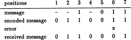
At the receiving end you apply the parity checks writing (from right to left) a 0 if the check is correct and a 1 if it is not. You get for the #1 check 0, for #2 a 1, and for #3 a 1. From right to left this is the binary number

$110\text{ which is decimal 6}$

so you change the digit in position 6, strip off the parity checks and you have the message.

This seems very inefficient for this short code, but a moment’s reflection will show you that for k parity checks you get a total message length of 2^k − 1 (of which k positions are used for the parity checks. Thus at k = 10, there are 1023 positions of which 1013 are useful message positions.

Exercises 2.10

2.10–1 In the code with n − 1 message positions and one check position what is the probability of no error? Ans. (1 – p)ⁿ

2.10–2 In example 1 if n = 1/p(large) what is the probability of no error? Ans. 1/e.

2.10–3 In the 2-out-of-5 code what is the probability of an error? Ans. C(5,1)pq⁴

2.10–4 In the 2-out-of-5 code what is the probabilty that two errors will not be detected?

2.10–5 In an error correcting code with k = 10, what is the probability of an undetected error? Note that all odd numbers of errors will be detected.

2.10–6 In the error correcting code if an additional parity check over the whhole message is added, show that double errors will be detected but will not be correctable.

2.10–7 In the code of Exercise 2.10–6 estimate the probability of an undetected error if p is small.

2.10–8 Discuss the wisdom of using the extra parity check (see Exercise 2.10–6) to detect double errors.

2.11  Summary

In Chapter 1 we introduced a simple model for the probability of an event based on symmetry, as well as several related ideas such as the sample space and randomness.

In this chapter we have developed the mathematical concepts needed to proceed, such as permutations and combinations, the binomial distribution, random variables, the mean and variance, generating functions and convolutions, and the weak law of large numbers which is central to the connection between the probability of a simple event and the frequency of occurence in a long run of identical and independent trials. We saw that the two concepts of probability, one based on symmetry and the other on the frequency of occurence, are not equivalent, that for the law to apply the variance must exist (but see Appendix 2.A).

In the next Chapter we will turn to developing five mathematical methods for solving problems. By examining the methods we will try to avoid Peirce’s condemnation of the reliability of solving probability problems; we will see the methods more clearly and become more familiar with their use and misuse.

Appendix 2.A Derivation of the Weak Law of Large Numbers

The weak law of large numbers was made to depend on the existence of the variance; it can be freed of this constraint as follows – though it still depends on the existence of the mean.

The approach is the classical one of the calculus; treat the infinite range as a finite range, compute the result, and then examine the result as the range is allowed to approach infinity.

The method is sometimes called the method of truncated variables and is quite useful in general. We assume we are looking at the average of n obervations of a random variable X. The expected value of X can be taken, for convenience, to be 0 since we could replace the random variable X by an new random variable X – μ, where μ is the mean. We regard the average (as before) as the average of n random variables X_i, (1 = 1, 2, …, n). To cope with the limit these variables X_i are then truncated

$\begin{array}{ccc}\{\begin{array}{l}{U}_i=X_i\\ U_i=0\end{array}& \{\begin{array}{l}{V}_i=0\\ V_i=X_i\end{array}& \begin{array}{l}\text{if }\left|X_i\right|\le kn\\ \text{if }\left|X_i\right|>kn\end{array}\end{array}$

where k is some (small) positive constant to be determined later. Thus we have for all i

$X_i=U_i+V_i$

To prove the weak law of large numbers we need to show that for any e > 0 both

$\begin{array}{l}P\left\{\right|U_1+U_2+\cdots +U_n|>\in n/2\}\to 0\\ P\left\{\right|V_1+V_2+\cdots +V_n|>\in n/2\}\to 0\end{array}$

Notice that we are considering only finite n; for any given e there is a corresponding n. Let the possible values of X_i be x₁, x₂, … and their corresponding probabilities be p(x_j). Then the expected value of | X_i| is

${\displaystyle \sum _j\left|x_j\right|p(x_j)=a}$

The bound on the U_i means that the x_j are also bounded, hence since the U_i are bounded by kn we can take one factor out and have

$E\left\{U_i^2\right\}\le kn{\displaystyle \sum _j\left|x_j\right|p(x_j)\le akn}$

The variables U_i all have the same probability distribution and are independent, hence

$V\{U_1+\cdots +U_n\}=nE\left\{U_i^2\right\}\le ak{n}^2$

But from the definition of the truncated variables as n → ∞

$E\left\{U_i\right\}\to E\left\{X_i\right\}=0$

Hence for sufficiently large n (since the X_i are independent the U_i are independent)

$E\left\{{(U_1+\cdots +U_n)}^2\right\}\le ak{n}^2$

We now apply the Chebyshev inequality to get

$P\left\{\right|U_1+\dots +U_n|>\in n/2\}\ge 8ak/{\in }^2$

and by choosing the k small enough our first requirement on the truncated variables is realized.

We now turn to the V_i have immediately

$P\{V_1+\cdots +V_n\ne 0\}\le nP\{V_i\ne 0\}$

For arbitrary k > 0 we have

$\begin{array}{l}P\{V_i\ne 0\}=P\left\{\right|x_i|>kn\}={\displaystyle \sum _{\left|x_i\right|>kn}p(x_i)}\\ \le (1/kn){\displaystyle \sum _{\left|x_i\right|>kn}\left|x_i\right|p(x_i)}\end{array}$

and this sum approaches 0 as n becomes infinite. Both terms approach zero so that the sum may be made as small as desired.

Appendix 2.B Useful Binomial Identities

Binomial identities play a large role in probability and other fields of mathematics, hence they are worth some attention. Since there are potentially an infinite number of identities among the binomial coefficients we will give only a few of the more useful ones.

From the definition

$\begin{array}{ll}C(n,k)\hfill & =\frac{n!}{k!(n-k)!}=\frac{n!(n-k-1)}{k(k-1)!(n-k+1)!}\hfill \\ \hfill & =\frac{(n-k+1)}{k}C(n,k-1)\hfill \\ C(n,0)\hfill & =1\hfill \end{array}$

(2.B-1)

we can compute the binomial coefficients recursively (as was used in (2.4–3)).

We often need the binomial coefficients for negative order. In the definition

$C(n,k)=\frac{n(n-1)(n-2)\dots (n-k+1)}{k!}$

we simply replace n by – n and get

$C(-n,k)=\frac{{(-1)}^k(n+k-1)(n+k-2)\dots (n)}{k!}={(-1)}^{k}C(n+k-1,k)$

(2.B-2)

If we multiply two binomial generating functions of different orders together we get

$\begin{array}{l}{(1+t)}^{m+n}={(1+t)}^m{(1+t)}^n\\ {\displaystyle \sum _{k}C(m+n,k)t^k}={\displaystyle \sum _{i}C(m,i)t^i}{\displaystyle \sum _{j}C(n,j)t^j}\end{array}$

(2.B-3)

Pick out the k^th power of t

$C(m+n,k)={\displaystyle \sum _{i}C(m,i)C(n,k-i)}$

For the special case m = n = k we get

$\begin{array}{ll}C(2n,n)\hfill & ={\displaystyle \sum _{i}C(n,i)C(n,n-i)}\hfill \\ \hfill & ={\displaystyle \sum _i{C}^2(n,i)}\hfill \end{array}$

(2.B-4)

In words, the sum of the squares of the binomial coefficients of order n is exactly the mid-coefficient of the expansion of order 2n.

Similarly identities like

$1+C(m+1,m)+C(m+2,m)+\cdots +C(m+n,m)=C(m+n,,m+1)$

are easily proved.