3

Methods for Solving Problems

“You know my methods, Watson.”

Sherlock Holmes

3.1    The Five Methods

It is widely believed that the only way to learn to do probability problems is by doing them. We have already used the method of “compute the complement” and the method of simulation. In this Chapter we will give and illustrate five widely used general methods for solving problems. They are:

1. Total sample space. First write out the total sample space.

(A) If the elementary events in the sample space are equally likely then the ratio of the number of successes to the total number of points in the sample space is the probability of a success.

(B) If the elementary events in the sample space have different probabilities then the probability of a success is the sum of all the probabilities of the elementary events that are successes.

We see that (A) is a very common special case of (B).

2. Enumerate. Enumerate (count) somehow only the equally likely successes and divide by the size of the total sample space to get the probability of a success (or add the probabilities of the successes).

3. Historical. Follow the history of the independent choices and take the product of the probabilities of the individual independent steps.

4. Recursive. Cast the problem in some recursive form and solve it by induction or recursion. This is often easiest done using state diagrams which are increasingly used in many parts of science. We shall develop and elaborate this method in Chapter 4.

5. Random Variables. In Section 2.5 we carefully introduced the idea of a random variable which conventionally written as X. It is used to indicate the value associated with the outcome of a general trial X (same label) whose possible outcomes are the points in the sample space. The outcomes are the x_k with probabilities p(k) and often having associated values that are simply k. Using the notation of Sections 2.5 and 2.6 we have for the expected value and variance (for x_k = k), (0 ≤ k ≤ K)

$\begin{array}{l}E\left\{X\right\}={\displaystyle \sum _{k=0}^{K}kp(k)=\mu }\\ V\left\{X\right\}={\displaystyle \sum _{k=0}^K{(k-\mu )}^{2}p(k)=E\left\{X^2\right\}-{[E\{X\}]}^2={\sigma }^2}\end{array}$

It is often easy to solve fairly complex problems using random variables (and a different frame of mind from the usual approach to probability problems).

We will first use a simple “occupancy” problem to illustrate the methods by solving the same problem by all five methods. Occupancy problems are the classic way of posing many probability problems—the standard form is: “In how many ways can a certain number of balls be put in a given number of places subject to the following restrictions?” The occupancy solution is readily converted to probabilities.

Example 3.1–1    The Elevator Problem (Five Ways)

The problem we will solve in this section is: suppose an elevator car has 3 occupants, and there are 3 possible floors on which they can get out. What is the probability that exactly 1 person will get out on each floor?

Since nothing else was said, we assume that each person acts independently of the others, and that each person has an equally likely chance of getting off at each floor. Without some such assumptions there can be no definite problem to solve. Of course different assumptions generally lead to different results.

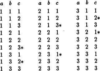
Method 1. Total Sample Space. We first create the total sample space. Let the people be labeled a, b and c, and list in some orderly fashion all possible choices of the exit floor for each person. One such ordering is shown in Table 3.1–1.

TABLE 3.1–1

Total Sample Space

The total sample space showing floor number (1, 2, or 3)

The 3³ = 27 different cases in the product sample space are all equally likely since we assumed both the independence of the people and the uniform probability choice for each floor. The six starred entries meet the criterion that all three floors are distinct, hence the probability we seek is

$6/27=2/9$

Method 2. Enumeration of Successes. In this method we write down only the 6 successes, (1, 2, 3), (1, 3, 2), (2, 1, 3), (2, 3, 1), (3, 1, 2), (3, 2, 1). We could also note that the number of ways of getting a success is exactly P(3,3) = 6. The total sample space is 3 × 3 × 3 = 27 (each person may choose any floor). Hence the probability sought is

$P(3,3)/3^3=6/27=2/9$

Method 3. Historical. In this method we trace the history of the elevator. For a success at the first floor only one person can get off. For the second stop there is again a probability of success. For the third similarly—hence the answer is the product of these three probabilities.

At the first floor if only one person gets off (and two do not) then, since there are 3 ways of choosing the person who gets off, we have 3[(1/3)(2/3)²] = 4/9. Using the earlier notation (2.4–2) we get the same result

$b(1;3,1/3)=C(3,1)(1/3){(2/3)}^2=12/27=4/9$

If we have a success at the first floor then at the second floor we have only two people left, and hence we have

$2(1/2)(1/2)=1/2$

or in the earlier notation

$b(1;2,1/2)=C(2,1)(1/2)(1/2)=2/4=1/2$

At the third floor the probability of success (assuming that the first two are successes) is exactly 1, hence for all three floors to be successes

$(4/9)(1/2)(1)=2/9$

as before.

Method 4. Recursive. To make the recursive method easy to understand we generalize the elevator problem to the case of n stops and n people. Let P(n) be the probability that exactly one person gets off at each of the n stops. Examining the first stop we have for a success on that floor that exactly one of the n persons gets off (with probability 1/n) and the other n − 1 do not get off (with probability [(n – l)/n]ⁿ − 1), then the recurrence formula is, since we have n − 1 persons left and n − 1 floors,

$\begin{array}{l}P(n)=(n)(1/n){[(n-1)/n]}^{n-1}P(n-1)={[(n-1)/n]}^{n-1}P(n-1)\\ P(1)=1\end{array}$

which is a simple recursion relation. From (2.4–2) we could have written the coeficient as b(1; n, 1/n) as we did the earlier ones.

We now unravel the recursion.

$\begin{array}{ll}P(n)\hfill & ={[(n-1)/n]}^{n-1}P(n-1)\hfill \\ \hfill & ={[(n-1)/n]}^{n-1}{[(n-2)/(n-1)]}^{n-2}\dots [1/2][1]\hfill \\ \hfill & =(n-1){[1/n]}^{n-1}(n-2)(n-3)\dots 1\hfill \\ \hfill & =(n-1)!/n^{n-1}=n!/n^n\hfill \end{array}$

For n = 1 this gives 1 as it should; for n = 2 we get 1/2 which is clearly correct as can be seen from the sample space of four points; and for n = 3 we get 6/27 = 2/9 as before. In some respects the general case is easier to solve than is the particular case of n = 3.

The general solution usually provides simple checks along the way to increase our confidence in the answer. If we use Stirling’s formula for the factorial (see Appendix 1.A) we get

$P(n)~e^{-n}\sqrt{2\pi n}$

and even at n = 3 the approximation is close. The following Table 3.1–2 indicates both: (1) how rapidly the approximation approaches the true value, and (2) how rapidly the probability approaches 0 as the number of floors increases.

TABLE 3.1–2

Elevator Problem

n	estimated	true	true – estimate
1	0.9221…	1.0000	0.0779…
2	0.4798…	0.5000…=1/2	0.0202…
3	0.2161…	0.2222…=2/9	0.0061…
4	0.0918…	0.0937…=3/32	0.0019…
5	0.0377…	0.0384…=24/625	0.0007…
6	0.0152…	0.0154…=5/324	0.0002…
7	0.0060…	0.0061…=6!/76	0.0001…
8	0.0024…	0.0024…=7!/87
9	0.0009…	0.0009…=8!/98
10	0.0004…	0.0004…=9!/109

This table gives us some feeling for the situation as a function of n, the number of floors.

The recursive method soon becomes the method of difference equations and leads to state diagrams, hence its importance is greater than it may seem now.

Method 5. Random Variables. We begin by assigning the random variable X to be 1 if at each floor only one person gets off and 0 otherwise. Thus the expected value of X will be the probability we want. Next we ask, “How can we break down this random variable into smaller parts?” Let the random variable Y_i(i = 1, 2, 3), be 1 if the ith floor is not used and 0 if it is. Then we have the key equation

$X=(1-Y_1)(1-Y_2)(1-Y_3)$

We now have

$\begin{array}{ll}P\hfill & =E\left\{X\right\}\hfill \\ \hfill & =E\{1-[Y_1+Y_2+Y_3]+[Y_1{Y}_2+Y_2{Y}_3+Y_3{Y}_1]-Y_1{Y}_2{Y}_3\}\hfill \\ \hfill & =1-[p(1)+p(2)+p(3)]+[p(1,2)+p(2,3)+p(3,1)]-p(1,2,3)\hfill \end{array}$

where

p(i)= probability that the ith floor is not used

P(i,j) = probability that both the ith and jth floors are not used

P(i,j,k) = probability that none of the floors is used.

The last sum is over distinct i, j and k, and is, of course, 0 since at least one floor must be used. We have

$\begin{array}{l}p(i)={(2/3)}^3\\ p(i,j)={(1/3)}^3\\ p(i,j,k)=0\end{array}$

Putting these in the formula we get

$P=1-3{(2/3)}^3+3{(1/3)}^3-0=1-8/9+1/9=2/9$

which is again the same answer.

The method of random variables seems to be a bit laborious in this simple example, but in section 3.6 we will give other examples which begin to show the power of the method. It should be clear that it requires a different way (art) of thinking, and that you need to learn how to pick wisely the random variables you define.

We now compare the five methods. When you can do the complete listing of the sample space it gives you a feeling of safety. When you try to enumerate the successes you are already a bit worried that you may have made an error. The historical approach also has some worries that you may have made an error but it seems to be relatively safe when you can use it. The recursive method, especially when you can generalize the problem, gives supporting checks of various cases and concentrates almost all the attention at two places, the setting up of the recurrence equation and the initial conditions. The random variable method is most effective in complex cases and has an elegance of method that makes it attractive once it is mastered. It seems to be relatively safe—when it works!

We next turn to the development of the five methods, and along the way we introduce a number of other useful ideas that arise in probability.

3.2    Total Sample Space and Fair Games

The method of laying out the total sample space and counting the successes is very simple to understand, hence in illustrating it we will introduce a new idea, that of a fair game.

A “fair game” is usually defined to be one in which your expectation of winning (probability of winning times the amount you can win) is equal to your expectation of losing (probability of losing times the amount you can lose). Thus for a fair game your total expectation is exactly 0. For example, betting a unit of money on the toss of a “fair” coin, Pr{H} = 1/2, and getting two units of money if you win (you win one unit) and none if you lose (you do not get your money back) is a fair game. Your total expectation is

$(1/2)(1)+(1/2)(-1)=0$

and it is by definition a fair game. There are in the literature much more elaborate and artificial definitions designed mainly to escape later paradoxes; we will stick to the common sense definition of a fair game.

Example 3.2–1    Matching Pennies (Coins)

A common game to consume time is “matching pennies” in which two players A and B each toss a coin (at random and independently). If the two coins show the same face then A wins (gets both coins), and if they are opposite then B wins. Supposing that the coins are each “well balanced” (meaning that the probability of a head is exactly 1/2) then the complete sample space is:

$\begin{array}{cccc}HH& HT& TH& TT\end{array}$

each with probability of 1/4. A wins on HH and TT so A has a probability of 1/2; so has B. Thus it is an unbiased trial and with the equal payoffs it is a fair trial.

We will use random variables to handle the repeated (independent) trials. Let X_i be the random variable that on the i^th toss A wins. It has the values

$X_i=\{\begin{array}{rr}\hfill 1& \hfill \text{win}\\ \hfill -1& \hfill \text{lose}\end{array}$

After n tosses we have the random variable S_n for the sum

$S_n=X_i+X_2+\cdots +X_n$

as the value of the game to A. It is easy to see from the total sample space that for each i the E{X_i) = 0, and V{X_i) = 1; each independent trial is fair and you either win or lose. Now for S_n we have

$\begin{array}{l}E\left\{S_n\right\}=0\\ V\left\{S_n\right\}=n\end{array}$

Since the expected value is 0 it is a fair game. Repeating a fair trial many times is clearly a fair game.

But by the law of large numbers (Section 2.8) it is the average, S_n/n, that probably approaches 0, not S_n. Indeed, we have already remarked that it is reasonable to estimate the deviation from the expected sum by an amount proportional to the square root of the variance (since the variance is the mean square of the deviations from the expected value). Hence we more or less “expect” that one player will have gained, and the other player lost, an amount about $\sqrt{n}$, though the expectation is 0. Yes, it is a fair game, but we “expect” that after n games one of the players will have lost approximately the amount $\sqrt{n}$ of money.

Example 3.2–2    Biased Coins

Suppose in Example 3.2–1 that the two coins are not exactly evenly balanced; rather that for the first coin the probability of a head is

$\begin{array}{cc}1/2+e_1& \left|e_1\right|<1/2\end{array}$

and for the second coin it is

$\begin{array}{cc}1/2+e_2& \left|e_2\right|<1/2\end{array}$

The probability that A wins—both coins are either heads or both tails—is now

$\begin{array}{l}(1/2+e_1)(1/2+e_2)+(1/2-e_1)(1/2-e_2)=\\ =1/2+2e_1{e}_2\end{array}$

and of course for B it is the complement probability 1/2 − 2e₁e₂.

In this case we see that the fairness of this game is not changed much by small biases in the coins—that the effect is of the order of the product of the two biases e_i, which should be quite small in practice. Such a result is said to be robust—that it is relatively insensitive to small changes in the assumed probabilities. Such situations are of great importance since in practice we seldom know that the probabilites in the real world are exactly what we assume they are in the probability model we use. See Section 3.9.

Example 3.2–3    Raffles and Lotteries

We consider first the simple raffle. In a raffle there may be several prizes, but for simplicity we will suppose that there is only one prize of value A (in some units of money). Let there be n tickets sold, each of unit value. What is your expected gain (assuming that each ticket has an equally likely chance of being drawn)? The probability, per ticket, is 1/n, so your expected gain G is

G = (A/n) (number of tickets you hold)—(cost of your tickets)

If the total number of tickets sold (yours plus the others) were exactly n = A, and if you hold k tickets, then your expected gain would be

$G=(k/n)[A]-k=k-k=0$

and it is “fair.” If more tickets are sold then it is “unfair to you” and if less then it is an “advantage to you.”

If you enter many similar “fair” raffles then according to the weak law of large numbers you will come close to balancing your losses and winnings, but the deviation between them will tend to go like $\sqrt{n}$.

To review, in a “fair game” your expectation of winning (per independent trial) is the same as the price you pay—the net expectation is zero. Otherwise it is “unfair” one way or the other. You may, of course, engage in a game that is unfair to you for purposes of amusement, or to “kill time,” and there are other reasons for buying raffle tickets—excitement, contributions to charity, easing your concience, obliging friends, etc. beyond just entering as a means of making money. As a general rule, there are far more tickets sold in a raffle than the value of the prize (prizes), and the raffle/lottery is thus unfair to you, but occasionally you see the opposite—due to charitable donations of prizes and/or the failure to sell enough tickets (possibly due to a stretch of bad weather) there may be a favorable raffle for you to enter.

In some kinds of lotteries it may happen that for several times no one has won the prize and it has accumulated. Thus it is conceivable that a lottery may be advantageous to you—but it is unlikely!

These are simple examples of looking at the total sample space; it is the number of tickets sold. Assuming the fair drawing of the tickets your chance of winning is the number you hold divided by the total sold (including yours). Your net expectation is this probability multiplied by the value of the prize minus your cost of buying tickets. This raises the following simple problem.

Example 3.2–4    How Many Tickets to Buy in a Raffle

Assuming: (1) the value of the prize is A, (2) that you know the number n of tickets sold (of unit cost), and (3) that you can buy as many as you wish at the last moment (and no one else can follow after you), then how many tickets should you buy?

Let the number to buy be k. After you buy k tickets then there are n + k tickets sold, and your probability of winning is k/(n + k). Your expectation of winning is Ak/(n + k), and your gain is

$G(k)=Ak/(n+k)-k$

We want to maximize G(k). We first assume that G(k) is a continuous function of k so we can apply the calculus (though we know it is discrete because we must buy a whole ticket at a time—still it won’t be far off, we hope). We can now scale the problem and isolate the size A of the prize. Using the value A of the prize as a measure, we introduce the relative number of tickets

$\begin{array}{l}\begin{array}{ccc}n/A=u,& \text{or}& n=uA\end{array}\\ \begin{array}{ccc}k/A=\upsilon & \text{or}& k=\upsilon A\end{array}\end{array}$

as new (relative) variables. We have, therefore, the corresponding continuous function

$G(\upsilon A)=\frac{A\upsilon A}{uA+\upsilon A}-\upsilon A=A\left[\frac{\upsilon }{u+\upsilon }-\upsilon \right]$

To find the maximum we set the derivative with respect to v (the variable of the problem; u is known) equal to zero.

$A{G}^{\prime }(\upsilon A)=A\left[\frac{(u+\upsilon )-\upsilon }{{(u+\upsilon )}^2}-1\right]=0$

We get, when we multiply through by the denominator,

${(u+\upsilon )}^2=u$

from which we get

$\upsilon =\sqrt{u}-u$

Going back to the original variables n and k we have the number of tickets to buy is

$k=A[\sqrt{u}-u]=A[\sqrt{n/A}-n/A]=\sqrt{nA}-n$

Since we are imagining that u < 1 (or else we are not interested in the raffle) we have v > 0. At this optimum the value (gain) of the raffle to us is, of course,

$\begin{array}{ll}G(\upsilon )\hfill & =A\left[\frac{\sqrt{u}-u}{u+\sqrt{u}-u}-\sqrt{u}+u\right]\hfill \\ \hfill & =A[1-\sqrt{u}-\sqrt{u}+u]=A{(1-\sqrt{u})}^2\hfill \\ \hfill & ={[\sqrt{A}-\sqrt{n}]}^2\hfill \end{array}$

We see that when u is near to 1, that is n is near A (the value of the tickets sold is almost the value of the prize) then the value of the raffle to us is very small indeed—especially if you look at the risk you take in making the investment.

For the original discrete variable problem in integers these answers are not exactly correct since we replaced the discrete problem by a continuous one and solved the new problem. For example, in the extreme case of n = 0 (no tickets sold) you should buy 1 ticket, but the formula indicates no tickets. When u = 1, namely n = A, there is no sense in buying a ticket since then your expectation for the first ticket is A/(n+1) = n/(n+ 1) and is less than what you will pay for the ticket. Indeed, at n = A − 1 it is doubtful that it is worth the effort, though the game is then fair.

Exercises 3.2

3.2–1. In Example 3.2–2 suppose that the two biases are exactly opposite, e₁ =—e₂. Discuss why the answer is what it is.

3.2–2 Consider Example 3.2–2 where only one coin is biased. What does this mean? Ans. The bias has no effect!

3.2–3 Discuss the case when there are several prizes in a raffle of varying values.

3.2–4 What is the probability of 3 or 1 heads on the toss of three biased coins? Discuss the solution. Ans. 1/2 + 4e₁e₂e₃, and at least one fair coin makes the game fair.

3.2–5 Solve Example 3.2–5 in integers by using G (k + 1) – G (k).

3.2–6 In the gold-silver coin problem (Example 1.9–1) suppose that there are three kinds of coins, gold, silver, and copper, with two to a drawer, and 6 drawers. Show that the probability of a gold coin on the second draw is 1/2.

3.2–7 In Example 1.9–1 suppose there are 4 drawers with GGG, GGS, GSS, and SSS. Show that the answer is still 2/3.

3.2–8 If A has 3 tickets in a raffle with 9 tickets sold, and B holds 1 in a raffle of 3, find the ratio of their probabilites of having a winning ticket.

3.2–9 If there are three prizes in a raffle and A holds 3 of exactly 9 tickets sold, what is the probability that A will not get any prize? Ans. 16/21.

3.2–10 On the roll of a die you win the amount of the face. If the game is to be fair what should you pay for a trial? Ans. 7/2.

3.2–11 You roll two dice and get paid the sum of the faces; what should you pay if it is to be fair?

3.2–12 You draw a card at random from a deck. If you get paid 1 unit for each face card and 2 units for an ace (and nothing otherwise) what is a fair price for the game? Ans. 5/13.

3.2–13 You toss 6 coins and win when you get exactly three heads. What is a fair price?

3.2–14 You roll a die and toss a coin. You get the square of the face of the die if and only if you got a head on the coin. What is a fair price?

3.2–15 You toss a coin and roll a die and are paid only if it is a H and a 4 that shows. What is a fair price? Ans. 1/12.

3.2–16 You roll three dice and are paid only if all three faces are even. What is a fair price?

3.3    Enumeration

In this method we do not try to lay out the whole sample space of equally likely cases; rather we compute its size and find only the successes.

Example 3.3–1    The Game of 6 dice

There is a game in which you roll 6 dice and you are paid according to the following rule:

if 1 face shows 6,	you win 1 unit
if 2 faces show 6,	you win 1 1/2 units
if 3 faces show 6,	you win 2 units
if 4 faces show 6,	you win 2 1/2 units
if 5 faces show 6,	you win 3 units
if 6 faces show 6,	you win 3 1/2 units

The argument (given by the gambler offering you the chance) for why you should play is that you expect that you will get at least one 6 on each roll of 6 dice, and all the higher ones are gains, so that if you pay 1 unit to play then it is favorable to you. But is it? (It is fairly safe to assume that any widely played game is favorable to the person running it and not to the player.)

Using the earlier notation (2.4–2) we have the probability for exactly k faces is

$b(k;6,1/6)$

From the above table the formula for the payoff for tossing k 6s

$\begin{array}{cc}1/2+k/2& (k=1,2,\dots 6)\end{array}$

The expectation of the sum of the payoffs is

$\begin{array}{l}{\displaystyle \sum _{k=1}^6(1/2+k/2)b(k;6,1/6)}\\ =(1/2){\displaystyle \sum _{k}b(k;6,1/6)}+(1/2){\displaystyle \sum _{k}kb(k;6,1/6)}\end{array}$

The first summation is (since the sum of all the probabilities from 0 to 6 is 1)

$\begin{array}{l}1/2[1-\text{the zeroth term]}=(1/2)[1-b(0;6,1/6)]\\ =1/2-(1/2){(5/6)}^6\\ =1/2-0.16745\dots \end{array}$

The second summation can be found from the generating function of the b(k;6,1/6), namely (2.4–5)

${(q+pt)}^6={\displaystyle \sum _{k=0}^{6}b(k;6,p)t^k}$

where p = 1/6 and q = 5/6. Differentiating with respect to t and setting t = 1 we get (the expected value)

$6p=1={\displaystyle \sum _{k=1}^{6}kb(k;6,1/6)}$

hence we have for the payoff

$1/2[1-b(0;6,1/6)]+1/2=1-0.16745\dots =0.83255\dots$

and the game is decidedly unfair to the player!

When you try to think about how this game can be unfair it may be confusing because the derivation is so slick. Hence to develop your intuition we write out some of the details in Table 3.3–1.

TABLE 3.3–1

The Six Dice Game

No. of 6s	probability
0	1(5/6)6	= .334 898 0
1	6(5/6)5(1/6)	= .401 877 6
2	15(5/6)4(1/6)2	= .200 938 8
3	20(5/6)3(1/6)3	= .053 583 7
4	15(5/6)2(1/6)4	= .008 037 6
5	6(5/6)(1/6)5	= .000 643 0
6	1(1/)6	= .000 021 4

We see that only about 40% of the time do we get exactly one 6 and come out even, while about 33% of the time we get no 6s at all! The gains for the multiple 6s do not equal the losses.

Perhaps why it is unfair is still not as clear as you could wish if you are to develop your intuition, so you do the standard scientific step and reduce the problem to a simpler one that appears to contain the difficulty. Consider tossing two fair coins, with payoffs of 1 for a single head and 3/2 for a double head. Now you have the simple situation

TABLE 3.3–2

The Two Coin Game

Outcome	probability	payoff
TT	1/4	0
TH	1/4	1
HT	1/4	1
HH	1/4	3/2

The total payoff (each multiplied by its probability of 1/4) is

$(1/4)[0+1+1+3/2)=(1/4)(7/2)=7/8$

and you see that it is again unfair. But this time it is so simple that you see clearly how the result arises—it is the failure to payoff properly on the two heads, which should be one unit per head tossed. With the 6 dice the situation is sufficiently complicated that you might get lost in the details and not see that it is the failure to payoff 1 unit for each 6 that causes the loss. The smaller payments, by advancing by 1/2 instead of 1 each time another 6 arises, is where the loss occurs. Since you expect one 6 on the average, you lose on the multiple cases where you are not paid 1 for each 6.

The problem of finding the successful cases among the mass of all possible cases closely resembles the problem of finding a good strategy in many AI (artificial intelligence) problems. The main difference is that in AI it is often necessary to find only one good solution, while we require finding all solutions that meet a criterion. Still, many of their methods may be adapted to our needs.

An example of an AI technique is “backtracking” which systematically eliminates many branches where it is not worth searching. We will illustrate the method by a simple problem.

Example 3.3–2    The Sum of Three Dice

What is the probability that the sum of the faces on three dice thrown at random will total not more than 7?

We begin by listing the canonical (increasing) representations in a systematic fashion. We start with the first two dice having faces 1,1, and then let the third one be in turn 1, 2, 3, 4, 5. We cannot allow 6 as the sum would be too large. We now “backtrack” and advance the immediately previous face to 2, thus we have 1,2 and start with the third die running through 2, 3, 4, and that is all. And so we go, and when one face cannot be advanced further we advance the immediately previous die face one more. In this way we generate the table of canonical representations

$\begin{array}{llllll}(1,1,1)\hfill & (1,1,2)\hfill & (1,1,3)\hfill & (1,1,4)\hfill & (1,1,5)\hfill & 13\hfill \\ (1,2,2)\hfill & (1,2,3)\hfill & (1,2,4)\hfill & \hfill & \hfill & 15\hfill \\ (1,3,3)\hfill & \hfill & \hfill & \hfill & \hfill & 3\hfill \\ (2,2,2)\hfill & (2,2,3)\hfill & \hfill & \hfill & \hfill & 4\hfill \\ \hfill & \hfill & \hfill & \hfill & \text{total}=\hfill & 35\hfill \end{array}$

This can be easily checked from Table 2.4–3.

These 11 are all the canonical cases that occur; we have only looked at about 5% of the 216 possible cases! We now multiply each canonical representation by its correct factor to get the number of equivalent representations out of the total 216 representations; as before if all three entries are the same then the factor is 1, if two are the same and one different then the factor is 3, and if all three are different then the factor is 6. We get the totals of each line on the right. The total number of possible outcomes is 6³ = 216, and each outcome has the same probability 1/216. The probability that the sum is not more than 7 is therefore 35/216 = 0.162….

Backtracking has clearly eliminated, in this case, a lot of the sample space as a place to search for successes. The use of the canonical representations reduced the initial number of cases from 35 to 11. In many problems backtracking, and similar methods from AI, can greatly simplify the search of the total sample space for the sucesses.

Exercises 3.3

3.3–1 If on rolling two dice you win your point when either die has the number or when their sum is your number, then what are the probabilities for winning for each point (1 through 12)? (Cardan)

3.3–2 Extend the gold coin problem of Example 1.9–1 and Exercise 3.2–3 to n coins in n + 1 drawers. Ans. 2/3.

3.3–3 Extend Exercise 3.3–2 to drawing k gold coins and then estimating the probabilty of the next being gold. Ans. (k + 1)/(k + 2).

3.3–4 Find directly the probability of the sum of three dice being less than or equal to 8. Check by Table 2.4–3.

3.3–5 Find the probability of the sum of four dice being less than or equal to 7

3.3–6 What is the probability of getting either a 7 or an 11 in the roll of two dice? Ans. 2/9

3.3–7 What is the probability of getting a total of 7 on the roll of four dice?

3.3–8 Using back tracking find a position on a chess board for which there are 8 queens each of which is not attacked by any other queen.

3.3–9 Find all such board positions asked for in Exercise 3.3–8.

3.3–10 If the face cards count J = 11, Q = 12, and K = 13 what is the probability of two random draws (with replacement) totaling more than 15?

3.3–11 Same as 3.3–10 except without replacement.

3.3–12 In the toss of 6 coins what is the probability of more than 3 heads?

3.3–13 In a hand of 13 cards four are aces. What is the probable number of face cards?

3.3–14 In Exercise 3.3–13 what is the probability of no face cards? Ans. C(36,9)/C48,9)

3.4    Historical Approach

Early in the correspondence between Fermat and Pascal (which is often said to have begun the serious development of probability theory) the problem of points was discussed. The question was: in a fair game of chance two players each lack sufficient points in order to win. If they must separate without finishing the game, how should the stakes be divided between them?

Example 3.4–1    The Problem of Points

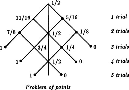
The historical approach, this time used bade wards, provides a convenient approach. We draw figure 3.4–1 for the case n = 3 as the number of points needed to win. The figure is the complete “tree” starting at the top with no trials made, and going to the left for each success of player A and to the right for a failure, each with the assumed probability of 1/2. At each level we have the situation after the indicated number of trials. The nodes that end with a win for A are marked with a payment of 1, and those for B are marked with 0, meaning that A gets nothing. We then “back up” the tree (as with a PERT chart) to get the values to assign earlier values (the average of the two descendant nodes). These derived values are marked on the nodes and give the value of the game to A at that position. At a symmetrical point (about the vertical middle line) the value for B is the complement (with respect to 1) of the marked value. The values for B are naturally the complements of those for A.

FIGURE 3.4–1

Example 3.4–2    Three Point Game With Bias

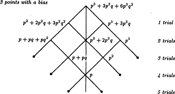
Suppose that in the game of points the probability is not 1/2 but rather A has a probability p of winning at each trial, and that the play is supposed to continue until one player has a total score of 3.

We again draw a “tree,” Figure 3.4–2, and mark the wins and losses as before. But this time when we “back up” the values we must consider the probabilities of the events. We get the indicated values for the game at each stage, including the interesting value at the top for the advantage A has at the start of the game. The coefficients of the terms at each node are actually the number of paths for reaching a win from that position, and the powers of p and q in the term are the number of steps in the corresponding directions.

FIGURE 3.4–2

This (backward this time) evolutionary approach to probability problems is very useful, and we have used it several times already. The above example shows a slight twist to the concept, examining how the winning positions can arise, and hence their probabilities.

Example 3.4–3    Estimating the Bias

If in the game of points one is forced to stop before the end, and if the outcome of a trial depends on skill rather than luck, then the ratio of successes to the total number of games so far played will give an indication of the probability p of a given player winning at a single trial. This has, of course, all the risk of any statistical estimate, but if the game depends on skill and you have no other data available to estimate the relative skills of the two players (at that moment in time), then what else is reasonable? Thus the ratio of games so far won to the total tried gives the estimates of the p to be used.

We have used the historical approach a number of times before, for example in the birthday problem, so more examples are not needed now.

Exercises 3.4

3.4–1 Show that Figures 3.4–1 and 3.4–2 agree.

3.4–2 Discuss interchanging p and q in Figure 3.4–2.

3.4–3 Work out the details for Example 3.4–3.

3.4–4 If there are 5 white balls and 4 black balls in an urn, what is the probability that on drawing them all out they will be alternating in color? Ans. p = 1/126.

3.4–5 In Example 3.4–3 show how the proposal tends to make small differences in ability into greater differences.

3.4–6 There are 6 discs numbered 1, …, 6. What is the probability of drawing them in a preassigned order? Ans. 1/6!

3.4–7 In drawing the six discs in the previous problem what is the probability that you will get all the even numbered ones before the odd numbered ones?

3.4–8 Previous problem with 2n discs. Ans. (n!)²/(2n)!

3.4–9 In a bag of 2 red, 3 white, and 4 black balls what is the probability that you will get all the red, then the white, and finally the black balls in that order?

3.5    Recursive Approach

The recursive method of solving probability problems is very powerful, and often gives both: (1) valuable cross checks, and (2) a feeling for why the particular case comes out as it does. It is, in a sense, the historical approach with a great deal of regularity.

Example 3.5–1    Permutations

The simplest example of the recursive method is the derivation of the number of permutations. If P(n) is the number of permutations of n things, then clearly you can pick any one of the n items and have left n − 1 items,

$\begin{array}{cc}P(n)=nP(n-1)& P(1)=1\end{array}$

We solve this recursion (difference equation) as follows:

$P(n)=n(n-1)P(n-2)=n(n-1)(n-2)P(n-3)=\cdots =n!$

Our attention is focused at just two places, the recurrence relation and the intital condition; we do not need to repeat the same argument again and again.

Example 3.5–2    Runs of Heads

What is the probability of a run of at least n heads? We have for a run of one head the probability p. This is a basis for the recursive approach. We assume that we have the probability P(n) of a run of n heads and ask for the probability of a run of n + 1 heads. It is clearly given by

$\begin{array}{cccc}P(n+1)=pP(n),& P(1)=p& \text{or}& P(0)=1\end{array}$

whose solution (see Appendix 4.A) is p(n) = pⁿ (using the first case to determine the arbitrary coefficient of the solution).

If the run is to stop at exactly n heads then the next outcome must be a tail and we have

$p^{n}q$

as the probability of exactly n heads. The sequence {pⁿq} is the distribution of exactly n successes.

In Example 3.2–2 we examined the probability of getting two or no heads with two biased coins. In Exercise 3.2–4 we examined the probability of three or one heads in three tosses of a biased coin. Hence we next look at the general case of N tosses of a coin and getting exactly N heads or less than N by an even number. This problem again illustrates the recursive method.

Example 3.5–3    N Biased Coins

Given N biased coins, P_i(H) = 1/2 + e_i, what is the probability P_N of the number of heads being either N or less than N by an even number? We solve it, naturally, by a recursive method. We have the cases N = 1,2, and 3 as a basis for the induction on the number of coins N. We have the recurrence equation describing a success at stage N based on the success or failure at stage (N − 1) coins,

$\begin{array}{ll}{P}_1\hfill & =1/2+e_1\hfill \\ P_N\hfill & =P_{N-1}(1/2+e_N)+(1-P_{N-1})(1/2-e_N)\hfill \\ \hfill & =(1/2)P_{N-1}+P_{N-1}{e}_N+1/2-(1/2)P_{N-1}-e_N+P_{N-1}{e}_N\hfill \\ \hfill & =(1/2)-e_N+2P_{N-1}{e}_N\hfill \end{array}$

If we set

$P_k=1/2+E_k$

where E_k is the bias at stage k of the induction (note E₁ = e₁). We have from the above equation

$1/2+E_N=1/2-e_N+2[1/2+E_{N-1}]e_N$

from which we get for the bias at stage N

$E_N=2e_N{E}_{N-1}$

The solution of this recurrence relation is

$E_N=2^{N-1}{e}_N{e}_{N-1}\dots e_1$

hence

$P_N=1/2+2^{N-1}{e}_1{e}_2\cdots e_N$

This solution checks for P₀ = 1, P₁ = 1/2+ e₁, and the previous results.

Note 1. If any one coin is unbiased, (some e_k = 0), then no matter how biased the other coins are (even if all the others are two headed or two tailed) the game is fair.

Note 2. If you change the rule to “an even (odd) number of heads” the answer changes at most by minus signs only.

Note 3. As long as some fraction of the coins have | e_k | < e < 1/2 then P_N → 1/2 as N → ∞. Notice that this does not involve the weak law of large numbers.

Example 3.5–4    Random Distribution of Chips

Suppose there are a men and b women, and that n chips are passed out to them at random. What is the probability that the total number of chips given to the men is an even number?

We regard this as a problem depending on n. We start with n = 0. The probability that the men have an even number of chips when no chips have been offered is (since 0 is an even number)

$P(0)=1$

How can stage n arise? From stage n − 1, of course. We have (similar to the previous example) the recurence equation

$P(n)=[b/(a+b)]P(n-1)+[a/(a+b)][1-P(n-1)]$

We write this difference equation in the cannonical form (see Appendix 4.A)

$P(n)-\frac{b-a}{b+a}P(n-1)=\frac{a}{b+a}$

For the moment we write

$(b-a)/(b+a)=A$

The difference equation is now

$P(n)-AP(n-1)=\frac{a}{b+a}$

The homogeneous difference equation

$P(n)-AP(n-1)=0$

has the solution (it can also be found by simple recursion)

$P(n)=C{A}^n$

for some constant C.

For the particular solution of the complete equation we try an unknown constant B as a guessed solution. We get

$B-AB=\frac{a}{b+a}$

or

$\begin{array}{c}B=\left(\frac{a}{b+a}\right)\frac{1}{1-A}=\left(\frac{a}{b+a}\right)\left[\frac{a+b}{a+b-(b-a)}\right]\\ =a/2a=1/2\end{array}$

Thus the general solution of the difference equation is

$P(n)=1/2+C{\left\{\frac{b-a}{b+a}\right\}}^n$

We now fit the initial conditions P(0) = 1. We get immediately that C = 1/2, and the solution is

$\begin{array}{c}P(n)=\frac{1}{2}\left[1+{\left\{\frac{b-a}{b+a}\right\}}^2\right]\\ =\frac{1}{2}\left[{\left\{\frac{b+a}{b+a}\right\}}^n+{\left\{\frac{b-a}{b+a}\right\}}^n\right]\end{array}$

which is more symmetric, and perhaps easier to understand.

To check the solution, we note that if a = 0, meaning there are no men, then certainly (meaning P(n) = 1) the number of chips given to them is an even number as the formula shows. If a = b then we have for all n > 0

$P(n)=1/2$

as it should from symmetry. Finally, if there are no women, b = 0, then

$P(n)=\frac{1+{(-1)}^n}{2}$

which alternates 0 and 1 as it should. Thus we have considerable faith in the solution obtained.

Example 3.5–5    The Gambler’s Ruin

Suppose gambler A holds a units of money and gambler B holds b units. If the probabilty of A winning on a single Bernoulli trial is p and they play until one of them has all the money, T = a + b, (T = total money) what is A’s chances of winning?

We begin with the observation that we are concerned with a probability P(n) if A holds exactly n units for all n (0 ≤ n < T) since all such states may arise in the course of the game. We set up the standard equation, which gives the probability of A being in the state of holding n units; namely by either winning one trial and going from holding n− 1 to holding n, or else by losing and going from holding n + 1 to holding n. The difference equation is clearly

$\begin{array}{cc}P(n)=pP(n-1)+qP(n+1)& (n=1,2,\dots ,T-1)\end{array}$

We next need the end conditions. When n = 0 (the gambler has no money, P(0) = 0) we know that A is certain to lose—A has no money to play. For n = T we know A is certain to win (B has no money to play) so P(T) = 1. Thus the end conditions are

$\begin{array}{ccc}P(0)=0,& \text{and}& P(T)=1\end{array}$

To solve the difference equation (in its standard form)

$qP(n+1)-P(n)+pP(n-1)=0$

we naturally try P(n) = rⁿ. This gives the characteristic equation (provided pq ≠ 0)

$q{r}^2-r+p=0$

whose roots are

$r=\frac{1\pm \sqrt{1-4pq}}{2q}$

We first look at the important special case of p = 1/2 = q. For this we have multiple characteristic roots

$r=1,1$

and the solution of the difference equation is

$P(n)=C_1+C_{2}n$

From P(0) = 0 we get C₁ = 0, and from P(T) = 1 we get C₂ = 1/T. Hence the solution is

$P(n)=n/T.$

Correspondingly A’s probabilty of ruin is 1 – n/T. At the start of the game (n = a, the original amount of money he had) this probability of winning is

$P(a)=\frac{a}{a+b}$

Of course B’s probabilties are the complements, (or interchange a and b).

We now return to the general case where p is not 0, 1/2, or 1. The term in the radical

$1-4pq=1-4p(1-p)=1-4p+4p^2={(1-2p)}^2$

so the characteristic roots are

$\{1\pm (1-2p)\}/2q=1,p/q$

Hence the general solution is

$P(n)=C_1+C_2{\left(\frac{p}{q}\right)}^n$

We need to fit the boundary conditions. For P(0) = 0 we get

$0=C_1+C_2\Rightarrow C_1=-C_2$

and for P(T) = 1 we have

$\begin{array}{l}1=C_2\left\{{\left(\frac{p}{q}\right)}^T-1\right\}\\ C_2=1/\left\{{\left(\frac{p}{q}\right)}^T-1\right\}\end{array}$

and

$P(n)=\left\{{\left(\frac{p}{q}\right)}^n-1\right\}/\left\{{\left(\frac{p}{q}\right)}^T-1\right\}$

At the start n = a and T = a + b and

$P(a)=\left\{{\left(\frac{p}{q}\right)}^a-1\right\}/\left\{{\left(\frac{p}{q}\right)}^{a+b}-1\right\}.$

The probability of ruin is the complement

$Q(n)=1-P(n)$

Alternately, A’s probability of losing is exactly B’s probability of winning.

For more material on the gambler’s ruin, such as the probable length of play, see [F, p.345ff].

Exercises 3.5

3.5–1 Suppose the game in Example 3.5–4 is changed to an even number for a win. Find the sign to be properly attached at each stage N.

3.5–2 Check algebraically that the last statement in this section is correct.

3.5–3 Discuss the cases in Example 3.5–5 when pq = 0.

3.5–4 If in Example 3.5–4 there are twice as many women as men what is the answer? Is it reasonable? If there are k times as many?

3.5–5 Discuss the convergence of the solution in Example 3.5–4 as the number of chips grows larger and larger.

3.5–6 Discuss the “drunken sailor” random walk along a line starting at x = 0. What is the probable distance from x = 0 after N steps?

3.5–7 The gamma function is defined by the integral ${\displaystyle {\int }_0^{\infty }{x}^{n-1}{e}^{-x}dx}$ For integral n find the recurrence formula and the value of the integral. Ans. (n − 1)!

3.5–8 Evaluate $L_n={\displaystyle {\int }_0^1{(\mathit{ln\hspace{0.17em}}x)}^n}$ by a recursion method.

3.5–9 The Catalan numbers are defined by C(2n, n)/(n + 1). Find the recursion formula and evaluate the first five numbers.

3.6    The Method of Random Variables

We illustrate this important method of random variables by several examples. We have already in this Chapter, Section 3.1 and Example 3.2–1, used this method.

Example 3.6–1    Pairs of socks

Suppose there are n pairs of socks in a dryer and you pick out k socks. What is the average number of pairs of socks that you will have?

Let the random variable X_i,j be defined by

$X_{i,j}=\{\begin{array}{ll}1\hfill & \text{if the }{i}^{\text{th}}\text{ and }{j}^{\text{th}}\text{ socks form a pair}\hfill \\ 0\hfill & \text{otherwise}\hfill \end{array}$

Let the i^th sock be drawn by chance; since there are now 2n − 1 socks left the probability that the jth sock will form a pair with it is 1/(2n − 1), that is

$P\left\{X_{i,j}\right\}=E\left\{X_{i,j}\right\}=\frac{1}{2n-1}$

Now let the random variable X be the sum

$\begin{array}{cc}X={\displaystyle \sum _{1\le i,j\le k}{X}_{i,j}}& (i\ne j)\end{array}$

hence we have

$\begin{array}{c}E\left\{X\right\}={\displaystyle \sum _{i,j}E\left\{X_{i,j}\right\}=\frac{C(k,2)}{2n-1}}\\ =\frac{k(k-1)}{2(2n-1)}\end{array}$

We make a small table of the values of E{X], both to check the formula and get a better understanding of how the problem depends on the parameters k and n.

TABLE 3.6–1

The Random Socks Problem

k\n	n = 1	n = 2	n = 3
k = 2	(2 × 1)/(2 × 1) = 1	(2 × 1)/(2 × 3) = 1/3	(2 × 1)/(2 × 5) = 1/5
k = 3	—	(3 × 2)/(2 × 3) = 1	(3 × 2)/(2 × 5) = 3/5
k = 4	—	(4 × 3)/(2 × 3) = 2	(4 × 3)/(2 × 5) = 6/5
k = 5	—	—	(5 × 4)/(2 × 5) = 2
k = 6	—	—	(6 × 5)/(2 × 5) = 3

Many of the values in the table agree with plain thinking. For larger values, if k = 2n (all the socks are drawn) we get

$E(X)=\frac{2n(2n-1)}{2(2n-1)}=n$

and we have n pairs of socks. If k = 2n − 1 (we leave exactly one sock) then we have

$E(X)=\frac{(2n-1)(2n-2)}{2(2n-1)}=n-1$

pairs of socks. Hence we decide that the answer is probably right.

Example 3.6–2    Problem de Recontre

This famous matching problem may be stated in many forms. At a dance n men draw names of the wives at random; what is the probability that no man dances with his wife? Or n letters and envelopes are addressed, and then the letters are put in envelopes at random; what is the probabilty that no letter is in its envelope? Again, at an office party where each person puts a gift in a bag and later draws at random the gift, what is the chance that no one will get the gift they put in? These are the same question as the probability of no match when turning up cards from two well shuffled decks of cards and asking for the probability of no match. Indeed, it is the same as calling the cards in order and looking for no match from a well shuffled deck. There are many other equivalent versions of the problem.

Let the random variable X_i be defined by

$X_i=\{\begin{array}{ll}1\hfill & \text{if the }{i}^{\text{th}}\text{ letter is in the }{i}^{\text{th}}\text{ envelope}\hfill \\ 0\hfill & \text{otherwise}\hfill \end{array}$

The random variable X we are interested in is defined by

$X={\displaystyle \prod _{i=1}^n(1-X_i)}$

which is 1 if no letter is in its envelope and 0 otherwise. We have, on expanding the product

$\begin{array}{l}X=1-{\displaystyle \sum X_i}+{\displaystyle \sum X_i{X}_j}-{\displaystyle \sum X_i{X}_j{X}_k}+\cdots \\ \begin{array}{c}E\left\{X\right\}=1-n\{1/n\}+C(n,2)\{1/n(n-1)\}-C(n,3)\{1/n(n-1)(n-2)\}+\cdots \\ =1-1+1/2!-1/3!-\cdots +(-1{)}^n/n!\\ ~1/e=0.367879\dots \end{array}\end{array}$

The probability of at least one letter in its proper place is

$1-E\left\{X\right\}~1-1/e=0.632120558\dots .$

The approach to the limiting value 1 − 1/e is very rapid as the following short table for at least one in the correct envelope shows;

TABLE 3.6–2

n	exact value
1	1.0
2	0.5
3	0.666667
4	0.625
5	0.633333
6	0.631944
7	0.631429
8	0.632118
9	0.632121
10	0.632121

Thinking about the table you soon realize that the larger n is the easier it is for any one letter to miss its envelope, but the more letters give more chances for at least one hit; the table shows that in this case the two effects almost exactly cancel each other, once n is reasonably large.

Example 3.6–3    Selection of N Items From a set of N

Evidently if we did not replace an item after drawing it then after N draws we would have the complete set. But with replacement after each draw we can anticipate getting some items several times and hence missing some others. How many can we expect to miss?

Let the random variable X_i be

$X_i=\{\begin{array}{ll}1\hfill & \text{if the }{i}^{\text{th}}\text{ item is not taken}\hfill \\ 0\hfill & \text{if the }{i}^{\text{th}}\text{ item is taken}\hfill \end{array}$

Therefore defining $X=X_1+X_2+\cdots +X_N$

$E\left\{X\right\}={\displaystyle \sum E\left\{X_i\right\}}$

But the X_i are interchangable, hence

$E\left\{X\right\}=NE\left\{X_i\right\}$

Now what is the probability of missing the ith item in the N trials? If each trial must miss then we have

${[(N-1)/N]}^N={[1-1/N]}^N~1/e=0.3678\dots$

(see Table 2.4–2). Hence the expected number of misses is

$N/e$

and we miss getting about 1/3 of the items when replacing each item immediately after each trial.

Exercises 3.6

3.6–1 Explain the oscillation in Table 3.6–2 in terms of the problem posed.

3.6–2 Give another example of the application of Example 3.6–2.

3.6–3 There are n sets of three matching items thrown in a bag. If you draw them out one at a time what is the expected number of matching sets?

3.6–4 In sampling n times with replacement what is the probability of getting all the items from a collection of n when is n = 1,2,3,…, n?

3.7    Critique of the Notion of a Fair Game

Galileo was once asked, “In estimating the value of a horse, if one man estimated the value at 10 units of money and the other at 1000 units, which of two made the greater error in estimating the value if the true value is 100 units of money?” After some consideration Galileo said that both were equally accurate, that it is the ratio of the estimate to the true value, rather than the difference, that is important.

To put the matter on a more personal level, suppose you have 1 million dollars and stand to either win or lose that amount on an even bet (p = 1/2). Most people do not feel that the gain in going from 1 million to 2 million dollars is as great as is the loss in going from 1 million dollars to nothing.

Thus we see that the definition of a fair game involving money, where the expectation of the loss is equal to the expectation of gain, does not represent reality for most people. Bernoulli faced this matter and suggested that the log of the amount you have after the gain or loss relative to what you had originally, is more realistic—but the log0 =—∞ and this may seem to be a bit too strong (so you might use the log of a constant plus the amount). Yet the log is not a bad measure to use in place of the amount itself. In any case we see that, except for very small amounts (small relative to the total amount possessed), the definion of a fair game is often not appropriate to life as we lead it. It has nice mathematical properties, that is true, but to apply it without thought of its implications is foolish; the concept needs to be watched very carefully when it is used in various arguments.

However, there is another side to the argument. People who engage in State Lotteries, when asked why they accept such unfavorable odds, give arguments (if they reply at all) such as, “Buying a ticket a week and losing each time will hardly change my life style, but if I win then it will make a great deal of difference to me,” Thus they feel that the slight loss in the expected value of their life style that they will suffer if they always lose is more than compensated for by the possibility (not the probability) that they will win a large amount on the lottery. They also often believe in a “personal luck” and not in the kinds of dispassionate, impersonal, objective probabilities that are expounded in this book.

One may also say about the usual concept of insurance, for the person taking out the policy there is a slight loss in the expected quality in their life (due to the premium paid) but a greatly reduced possible loss. Gambling may be viewed as the opposite of insurance, for a moderate loss in the expected value, the possible gain in their life is greatly raised. These opinions are to be considered more on an emotional level than on a rational level since we cannot know the nonmeasureable values attributed to them by the individual making the choice.

As we will show in Section 3.8, using the Bernoulli evaluation, the log of the amount of money posessed, leads to the reasonable results that gambling in fair games is foolish, and that ideally (no overhead) insurance is a good idea. Bernoulli used the log of the amount as the evaluation function, but it will be easy to see that any reasonable convex function would give similar results.

While we have just argued that the Bernoulli value of money, or some similar function, is the proper one to use when dealing with money, it does not follow that for other quantities, such as time, it is appropriate. In each case we must examine the appropriateness of using the expected value as the proper measure before acting on a computation involving the expected value.

3.8    Bernoulli Evaluation

In this section we give several examples of the Bernoulli evaluation of a fair game.

Mathematical Aside: Log Expansions. We often need the following simple results. From the expansion (that can be found by simple division if necessary)

$\begin{array}{cc}1/(1-x)=1+x+x^2+x^3+\cdots & (|x|<1)\end{array}$

we can integrate (from 0 to x) to get (recall that ln1 = 0)

$\mathit{ln\hspace{0.17em}}(1-x)=-(x+x^2/2+x^3/3+\cdots )$

(3.8–1)

Replace x by—x to get

$\mathit{ln\hspace{0.17em}}(1+x)=x-x^2/2+x^3/3-\cdots$

(3.8–2)

Subtract (3.8–1) from (3.8–2) to get

$\mathit{ln\hspace{0.17em}}\{(1+x)/(1-x)\}=2(x+x^3/3+x^5/5+\cdots )$

(3.8–3)

You can, if you wish, use finite expansions with a remainder in all the above, and finally go to the limit; the result will be the same.

Example 3.8–1    Coin Toss

Let p = 1/2 for a fair game with a gain or loss of one unit of money on the toss. Then the value of the game according to Bernoulli is, if you have N units of money at the start, (V_B = value Bernoulli)

$V_B=\frac{1}{2}\mathit{ln\hspace{0.17em}}(N+1)+\frac{1}{2}\mathit{ln\hspace{0.17em}}(N-1)$

The change in your value (you had ln N value before the game) by the toss is

$\begin{array}{l}\Delta V_B=\frac{1}{2}[\mathit{ln\hspace{0.17em}}(N+1)+\mathit{ln\hspace{0.17em}}(N-1)-2\mathit{ln\hspace{0.17em}}(N)]\\ =\frac{1}{2}[\mathit{ln\hspace{0.17em}}(1+1/N)+\mathit{ln\hspace{0.17em}}(1-1/N)]\\ =\frac{1}{2}\mathit{ln\hspace{0.17em}}(1-1/N^2)<0\end{array}$

Hence by (3.8–1) there is approximately a change of − 1/2N² in your value, and it is foolish (in an economic sense) to play the game.

From the previous example we can fairly easily see that if the payoff is symmetric in a fair game then each matching pair in the payoff is unfavorable, hence repeated trials are also unfavorable, and playing the game repeatedly is foolish. We show this in more detail in the next Example.

Example 3.8–2    Symmetric Payoff

For the toss of three coins (the order of the coins does not matter) let the payoff be the number of heads minus the number of tails, and suppose you start with N units of money.

outcome	payoff	probability
HHH	3A	1/8
HHT	A	3/8
HTT	–A	3/8
TTT	–3A	1/8

Is the game fair both in the classical sense and in the Bernoulli sense?

The game is clearly fair in the classical sense. However, the change in the Bernoulli value is

$\begin{array}{c}\text{change}=\frac{1}{8}[\mathit{ln\hspace{0.17em}}(N+3A)+\mathit{ln\hspace{0.17em}}(N-3A)]+\\ \frac{3}{8}[\mathit{ln\hspace{0.17em}}(N+A)+\mathit{ln\hspace{0.17em}}(N-A)]-\mathit{ln\hspace{0.17em}}N\\ =\frac{1}{8}[\mathit{ln\hspace{0.17em}}\{1-(3A/N{)}^2\}+3\mathit{ln\hspace{0.17em}}\{1-(A/N{)}^2\}]\end{array}$

and by 3.8–1 this is negative.

We are now ready to look at the general case of a fair game.

Example 3.8–3    Fair Games

If you have N units of money and

$\begin{array}{l}p=\text{probability of winning }A\text{ units}\\ \begin{array}{cc}q=\text{probability of losing }B\text{ units,}& (B<N)\end{array}\end{array}$

then for a classic fair game you must have

$pA=qB=C$

and the net gain (Bernoulli) is

$\begin{array}{c}\text{Gain}(N)=G(N)=p\mathit{ln\hspace{0.17em}}(N+A)+q\mathit{ln\hspace{0.17em}}(N-B)-\mathit{ln\hspace{0.17em}}N\\ =p\mathit{ln\hspace{0.17em}}(1+A/N)+q\mathit{ln\hspace{0.17em}}(1-B/N)\end{array}$

To study the function G(N) as a function of N we note that G(∞) = 0 regardless of the other parameter values p, g, A, and B. Next we examine the derivative with respect to N

$\begin{array}{ll}{G}^{\prime }(N)\hfill & =p\left[\frac{\frac{-A}{N^2}}{1+\frac{A}{N}}\right]+q\left[\frac{{\frac{B}{N}}^2}{1-\frac{B}{N}}\right]\hfill \\ \hfill & =\frac{1}{N}\left[\frac{-C}{N+A}+\frac{C}{N-B}\right]\hfill \\ \hfill & =\frac{C}{N}\left[\frac{1}{N-B}-\frac{1}{N+A}\right]\hfill \\ \hfill & =\frac{C}{N}\left[\frac{A+B}{(N-B)(N+A)}\right]>0\hfill \end{array}$

The derivative is always > 0, hence the curve must be rising, and since it is 0 at infinity we must have, for all finite N,

$\begin{array}{cc}G(\text{finite})<0& (\text{for }N>B)\end{array}$

Example 3.8–4    Insurance (Ideal—no Extra Costs)

In the insurance case, you are already in the game of life and you stand to lose an amount A < N (Where N = your total assets) with some probability p. In this game of life your current Bernoulli value is

$p\mathit{ln\hspace{0.17em}}(N-A)+q\mathit{ln\hspace{0.17em}}N$

If you took out insurance so that you would get back the amount A, then a (classical) fair fee would be (ideally)

$pA$

and your Bernoulli value would then be

$\mathit{ln\hspace{0.17em}}(N-pA)$

Computing the gain in taking the insurance

$\text{(insurance)}-(\text{no insurance})$

you get the gain

$\begin{array}{c}G(N)=\mathit{ln\hspace{0.17em}}(N-pA)-[p\mathit{ln\hspace{0.17em}}(N-A)+q\mathit{ln\hspace{0.17em}}N]\\ =\mathit{ln\hspace{0.17em}}(N-pA)-p\mathit{ln\hspace{0.17em}}(N-A)-(1-p)\mathit{ln\hspace{0.17em}}N\\ =\mathit{ln\hspace{0.17em}}(1-pA/N)-p\mathit{ln\hspace{0.17em}}(1-A/N)\end{array}$

Again we observe that

$G(\infty )=0$

but this time

$\begin{array}{c}{G}^{\prime }(N)=\frac{\frac{pA}{N^2}}{1-p\frac{A}{N}}-\frac{\frac{pA}{N^2}}{1-\frac{A}{N}}\\ =\frac{pA}{N}\left[\frac{1}{N-pA}-\frac{1}{N-A}\right]\\ =\frac{pA(-qA)}{N(N-A)(N-pA)}<0\end{array}$

Hence the curve always falls as a function of N, and therefore the function values must have been positive. Thus taking insurance is always good (assuming no overhead and that the insurance is priced fairly!).

Since there are actually fixed overheads in insurance policies the results must be slightly modified. It is easy to see that if your N is large it does not pay you to insure against a small loss, but when the loss is near to N is generally pays to take insurance. As a result the richer people tend to have fewer insurance policies than do the poorer people.

An examination of the last two proofs shows that any reasonable convex function that is differentiable in place of the log would not change the results. Hence the Bernoulli (log) value of money is not essential to the conclusions. The conclusion is that the classical “fair game” involving money is simply not “fair” will still hold for convex value functions. Thus the wide spread use of the expected value in probability can, at times, be grossly misleading.

Exercises 3.8

3.8–1 For the roll of a die if the payoff is 6 units for “hitting your point” show that the game is fair but the Bernoulli evaluation is not.

3.8–2 For the toss of a coin twice with (in order) HH payoff 2A, HT payoff A, TH payoff—A and TT payoff —2A, show that the game is fair but the Bernoulli evaluation is not.

3.8–3 What would the payoff have to be in a coin toss for the Bernoulli value to be zero? Note that it involves your present value.

3.8–4 Can a game be both fair and have a Bernoulli evaluation of zero?

3.8–5 Calculate the Bernoulli value of 2n fair games.

3.8–6 Replace the log N value with log(N + 1) and carry out the details, thus avoiding the infinite value when ending up with nothing.

3.9    Robustness

As you have seen, the first modelling of a situation often asumes that the probability distribution is uniform. It may in fact be only close to uniform distribution, so it is natural to ask how much the answer changes and in what direction it changes if there are slight differences from uniform in the distribution assumed. This is usually called “robustness” of the model, or “sensitivity” if you prefer. If we are to use the results of a probability computation in many practical situations we must not neglect this important aspect of practical mathematics. We will take the birthday problem of Example 1.9–6 as an example.

Example 3.9–1    The Robust Birthday Problem

Suppose that the distribution of birthdays in the year is not uniform, but assume that the probabilities deviate from 1/365 by small amounts e_i, that is (still using 365 days in the year and neglecting leap years) the probability of being born on the i^th day of the year is

$\begin{array}{cc}{p}_i=1/365+e_i& (i=1,2,\dots 365)\end{array}$

(3.9–1)

For generality we replace 365 by an arbitrary n.

We have, of course,

${\displaystyle \sum _i{e}_i=0}$

(3.9–2)

Therefore

${({\displaystyle \sum _i{e}_i})}^2=0$

by expanding the square of the series and transposing the squared terms we have the important relationship

${\displaystyle \sum _{i\ne j}{e}_i{e}_j}=-{\displaystyle \sum _i{e}_i^2}$

(3.9–3)

Now the probability we seek P_m for no duplicate birthdays in m choices must be a symmetric function in the e_i and consist of all terms of the form

$p_{i(1)}{p}_{i(2)}\cdots p_{i(m)}$

such that i, j ≠ i, k, for j ≠ k. We make a Taylor expansion in the variables e_i of this function P_m (P_i) about the values e_i = 0. We have

$P_m=P_m(1/n)+{{\displaystyle \sum d{P}_m/d{p}_i}|}_{1/n}{e}_i+{{\displaystyle \sum {\displaystyle \sum d^2{P}_m/d{p}_{i}d{p}_j}}|}_{1/n}{e}_i{e}_j+\cdots$

We now note that due to symmetry all the

${d{P}_m/d{p}_i|}_{1/n}=\text{same number for all }i$

hence

${{\displaystyle \sum d{P}_m/d{p}_i}|}_{1/n}{e_i=d{P}_m/d{p}_i|}_{1/n}{\displaystyle \sum e_i=0}$

by (3.9–2).

For the next term, the second derivatives evaluated at 1/n, we have for i ≠ j,

${d^2{P}_m/d{p}_{i}d{p}_j|}_{1/n}=\{\begin{array}{ll}1/n^{m-2}\hfill & \text{if both }{p}_i\text{ and }{p}_j\text{ are there}\hfill \\ 0\hfill & \text{otherwise}\hfill \end{array}$

and that

$d^2{P}_m/d{p}_i^2=0\text{ always}$

Hence

$P_m(p_i)=P_m(1/n)+(1/n^{m-2}){\displaystyle \sum e_i{e}_j}+\cdots$

Using (3.9–3) we get, finally,

$\begin{array}{c}{P}_m(p_i)=P_m(1/n)-(1/n^{m-2}){\displaystyle \sum e_i^2}+\cdots \\ =(\text{original answer})-(1/n^{m-3})\text{Var}\left\{e_i\right\}+\cdots \end{array}$

and we have found the major correction term in a very convenient form.

The equations (3.9–2) and (3.9–3) are the key ones in the reduction to the simple form; for such a symmetric problem the first order term will always cancel out, and the cross derivatives can sometimes be reduced to the second order ones and then the variance will emerge as the measure of the main correction term. We have, therefore, a convenient way of attacking the robustness of many symmetric problems when small deviations from the uniform distribution occur. For other kinds of problems we will need other tools, but equations (3.9–2) and (3.9–3) remain central.

The birthday problem is one of sampling with replacement; we next look at the elevator problem (Section 3.1) which samples without replacement and has a double index probability distribution.

Example 3.9–2    The Robust Elevator Problem

Looking back at the first solution (or the second one) we can take the six successes from the sample space

a1	b2	c3
a1	b3	c2
a2	b1	c3
a2	b3	c1
a3	b1	c2
a3	b2	c1

and compute their total probability as the probability of a success. Let the probability of the ith person getting off on the j^th floor be

$\begin{array}{cccc}p(i,j)& \text{with}& {\displaystyle \sum _{j=1,2,3}p(i,j)=1}& (\text{for }i=1,2,3)\end{array}$

This sum merely says that the ith person gets off on some floor.

For use as perturbations we set

$\begin{array}{cc}p(i,j)=1/3+e(i,j)& (\text{all }i\text{ and }j)\end{array}$

with

$\begin{array}{cc}{\displaystyle \sum _{j=1,2,3}e(i,j)=0}& (i=1,2,3)\end{array}$

(3.9–4)

The total probability is the sum of six terms of the form

$p(1,i)p(2,j)p(3,k)=[1/3+e(1,i)][1/3+e(2,j)][1/3+e(3,k)]$

To get the Taylor series expansion of the sum we need the derivatives with respect to the e(i,j) evaluated at e(i, j) = 0. We have

$\begin{array}{l}P(0)=6/27=2/9\\ \frac{dP(0)}{de(i,j)}=A=1/9\\ \begin{array}{cc}\frac{d^{2}P(0)}{de(i,j)de(k,m)}=B=1/3& (i\ne k,j\ne m)\end{array}\\ \frac{d^{2}P(0)}{de{(i,j)}^2}=0\end{array}$

The Taylor expansion is, therefore, since again the first order terms must cancel,

$P(e)=\frac{2}{9}+\frac{1}{2}\left(\frac{1}{3}\right){\displaystyle \sum _{i\ne k,j\ne m}e(i,j)e(k,m)}$

If we sum on the m for fixed i, j, k we have from (3.9–4)

${\displaystyle \sum _{m\ne j}e(i,j)e(k,m)=-e(i,j)e(k,j)}$

as a partial simplification for the expression. We can also write it in the form

$P(e)=\frac{2}{9}+\frac{1}{6}\{{\displaystyle \sum e_i,j{e}_k,m}-{\displaystyle \sum e_{i,j}^2\}}$

But we cannot reduce it to a sum of squares as the following argument shows. Consider the case p(1,1) = p(2,2) = p(3,3) = 1. Then P = 1, success is certain. Next consider the case, p(1,1) = 1 = p(2,1). Then P = 0, and failure is certain. Thus the surface in the perturbation variables e(i,j) has a saddle point (as can be seen by considering slight changes towards the two solutions indicated). Still, we have a formula for the change due to small changes in the probabilites (we have neglected any correlations that might also occur in practice). We see that again the change is quadratic in the perturbations, as one would expect from local extreme in a symmetric problem. But see [W].

We gave a rather general approach to robust problems and illustrated it by the birthday problem in Example 3.9–1. We now give an approach based on a variant of the birthday problem.

Example 3.9–3    A Variant on the Birthday Problem

Let N be the number of people entering the room, one at a time, until you have a 50% chance of a duplicate birthday. This differs from the earlier version of the birthday problem not only because it poses a different question but it also differs in the amount of effort to do a simulation. The question asked concerns the median value which is often quite different from the expected value.

To handle this problem this time we define the random variable X_j (for 0 < j < 366)

$x_J=\{\begin{array}{ll}1\hfill & \text{when }N>j\hfill \\ 0\hfill & \text{otherwise}\hfill \end{array}$

Consequently the number of people N until we get as 50–50 chance of a duplicate birthday is given by

$N=X_0+X_1+\cdots +X_n$

Next we take the expected value

$E\left\{N\right\}=1+p_1+p_2+\cdots +p_n$

where, as before,

$p_j=\left\{1-\frac{0}{365}\right\}\left\{1-\frac{1}{365}\right\}\cdots \left\{1-\frac{j-1}{365}\right\}$

Using a programmable hand computer we get E{N} = 24.617…

We next examine the variance of N in this formulation of the question. Note that since $X_i^2=X_i,$

$\begin{array}{c}{N}^2=X_0^2+X_1^2+\cdots +X_n^2+2{\displaystyle \sum _{i<j}{X}_i{X}_j}\\ =X_1+X_2+\cdots +X_n+2{\displaystyle \sum _{i<j}{X}_i{X}_j}\end{array}$

Now the random variables were cleverly chosen so that for i < j

$X_i{X}_j=X_j$

Therefore

$N^2=X_0+X_1+\cdots +X_n+2{\displaystyle \sum _{i=0}^{n-1}{\displaystyle \sum _{j=i+1}^n{X}_j}}$

and it follows that

$\begin{array}{ccc}E\left\{N^2\right\}=E\left\{N\right\}+2{\displaystyle \sum _{i=0}^{n-1}{r}_i}& \text{where}& r_i=p_{i+1}+\cdots +p_n\end{array}$

This formula also provides a way of computing when the probabilities of birthdays are not uniform over the year.

As an example of unequal probabilities of a birth on the various days of the year let p_i = 1/365 + Asin{(k − 1)2π/365} with k = 1, 2,… 365. This is a reasonable model if you think there is a periodic effect in the course of the year. With A = 0.002 (note that 1/365 = 0.00274) this is a huge amplitude oscillation which produces an approximate variation of 73% in some of the daily probabilities. The result of computation is that the expected number is now

$E\left\{N\right\}=24.6$

(which differs from the earlier uniform case only slightly. We have also

$\begin{array}{cc}E\left\{N^2\right\}=754.6166\dots & \text{Var}\left\{N\right\}=148.65\end{array}$

hence

$r=12.19\dots$

The effect of the large change from the uniform case is not as much as you might expect because the sum of the perturbations in the probabilities must total 0 and this produces, in almost all probability problems, a great deal of cancellation.

Example 3.9–4    A Simulation of the Variant Birthday Problem

The result of Example 3.9–3 may be checked by some simulations of the situation. The average number N over 100 trials gave the numbers

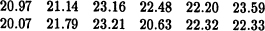
The average of these simulations is 22.0 vs. the calculated 24.6 but the variance is large.

3.10  Inclusion-Exclusion Principle

We first introduce the concept of an indicator variable on a set X. The variable is 1 when the point is in the set and is 0 otherwise. Thus for indicator variables X_i the quantity

$X_i{X}_j$

is 1 only when the point is in both sets X_i and X_j. Similarly for higher order products of indicator variables. We have used this notation before.

Suppose we have a number of sets A_i, some of which may overlap others. If we add all the A_i we will at least double count the common points, labeled A_i,j, see Figure 1.7–2. Hence we need to subtract these out. But then we will have twice removed all the points that occur in three sets at once and we need to add them back again, that is add A_i,j,k. Hence to count all the points in some set we have

$A={\displaystyle \sum A_i}-{\displaystyle \sum A_{i,j}}+{\displaystyle \sum A_{i,j,k}}-\cdots$

Figure 1.7–2 illustrates this situation for three sets using circles as sets. We now convert this to the indicator variables where where there is at least one point in the set X

$X={\displaystyle \sum X_i}-{\displaystyle \sum X_i{X}_j}+{\displaystyle \sum X_i{X}_j{X}_k}-\cdots$

Since combinations are often difficult for the beginner, we will proceed slowly and derive this formula in a different manner. We begin with the classical formula from algebra, the factoring of a polynomial in terms of the roots x_i. We have the standard formula

$\text{Poly }(x)=P_n(x)=(x-x_1)(x-x_2)\cdots (x-x_n)$

If we multiply this out and note that the terms in each coefficient of x^k are homogeneous (same degree) in the x_i we find that the term with no x_i is

$x^n$

The next term is x^n-1 and the coefficient is, by symmetry,

$-{\displaystyle \sum _i{x}_i}$

The next term’s coefficient is

$+{\displaystyle \sum _{i,j}{x}_i{x}_j}$

Indeed we see that P_n (x) will be

$P_n(x)=x^n-x^{n-1}{\displaystyle \sum x_i+x^{n-2}}{\displaystyle \sum x_i{x}_j-x^{n-3}}{\displaystyle \sum x_i{x}_j{x}_k}+\cdots$

with alternating signs and the last term will be the product of all the x_i with a coefficient (-1)ⁿ. The coefficients are called the elementary symmetric functions of the roots x_i.

If we set x = 1 and think of the x_i as indicator variables X_i we have

$(1-X_1)(1-X_2)\dots (1-X_n)$

If any X_i = 1 then the product is 0. Alternately for

$1-(1-X_1)(1-X_2)\dots (1-X_n)$

this is 1 if any X_i = 1. Expanding this we have

$1-1+{\displaystyle \sum X_i}-{\displaystyle \sum X_i{X}_j}+\cdots ={\displaystyle \sum X_i}-{\displaystyle \sum X_i{X}_j}+{\displaystyle \sum X_i{X}_j{X}_k}-\cdots$

this is the same formula as before in a slightly different notation, and we have already used it several times!

Example 3.10–1  Misprints

A common situation is that two readers independently examine a table of numbers. The first observes n₁ errors, the second n₂ errors, and in comparing the two lists of errors there are nz errors in common. How many errors are probably left?

We must, of course make some assumptions. The simplest are: (1) that each error has the same probability of being found as any other, (2) that the errors are independent, and (3) that the two readers have different probabilities of finding the errors. Let p(1) be the probability of the first reader finding an error and p(2) for the second. If there are N errors in total then reasonable estimates (not certain knowledge at all) are

$\begin{array}{ccc}p(1)=n_1/N& \text{and}& p(2)=n_2/N\end{array}$

We have for the common errors (they were assumed to be independent)

$p(1)p(2)=n_3/N$

This leads to, eliminating the p’s,

$n_1{n}_2=N{n}_3\Rightarrow N=n_1{n}_2/n_3$

This seems to be a reasonable result as we inspect it. If there were no errors found in common, (and nothing else was known about the reliability of the readers) the assumption of an infinite number of errors (though the text must have been finite) is not surprising. Other tests also show that it is a reasonable result for a first guess.

We have not answered the original question—how many are left. We need the inclusion-exclusion principle to get it. We have for the number of errors left the reasonable guess

$N-n_1-n_2+n_3$

The model is crude, of course, but it is suggestive, and if this number is too large for publication then further readers had better be found.

Example 3.10–2  Animal Populations

It is a common problem that we want to sample an animal (or other) population and guess at the total population N from the samples. Suppose we sample, count, and tag all the animals caught in this first sample, and return them to the original population. At a later date we sample again and count both the size and the number of tagged ones. Again we are estimating the total population (above it was errors in a table) and have labeled it as N. Let the n_i be as before. Then the total population N is estimated by

$N=n_1{n}_2/n_3$

One worries about the assumption of the independence of being captured twice. Are the trials really independent? Is there a tendency for some animals to be caught and other to escape? Does the presence of a tag change the probability of being caught again, or of survival to be later caught? Hence the need for robustness.

Example 3.10–3  Robustness of Multiple Sampling

The formula we are using is

$N=n_1{n}_2/n_3$

If each of these numbers has a small error e_i (i = 1, 2, 3) what can we expect for the change in N?

It is simple numerical analysis where we omit all squares and higher powers of the e_i. We have for the first order terms in the e_i.

$\begin{array}{ll}\text{Change}\hfill & =(n_1+e_1)(n_2+e_2)/(n_3+e_3)-n_1{n}_2/n_3\hfill \\ \hfill & ~[(n_1{n}_2+n_1{e}_2+n_2{e}_1)/n_3]\{1-e_3/n_3\}-n_1{n}_2/n_3\hfill \\ \hfill & ~n_1{e}_2/n_3+n_2{e}_1/n_3-n_1{n}_2{e}_3/n_3^2\hfill \end{array}$

This could also be found by a Taylor expansion to first order terms.

Example 3.10–4  Divisibility of Numbers

A number is chosen at random from the range of 30M + 1 to 30N(N > M); what is the probability that it will have no factors of 2, 3, or 5?

Clearly we first need to find how many numbers in the range are divisible by 2, 3 and 5. We have

$\begin{array}{l}\begin{array}{cc}\text{divisible by 2}& 30(N-M)/2=15(N-M)\end{array}\\ \begin{array}{cc}\text{divisible by 3}& 30(N-M)/3=10(N-M)\end{array}\\ \begin{array}{cc}\text{divisible by 5}& 30(N-M)/5=6(N-M)\end{array}\end{array}$

etc.

We must use the inclusion-exclusion principle, hence we have in all that are divisible by 2, 3 or 5

$\begin{array}{l}30(N-M)\left\{\frac{1}{2}+\frac{1}{3}+\frac{1}{5}-\left\{\frac{1}{6}+\frac{1}{10}+\frac{1}{15}\right\}+\frac{1}{30}\right\}\\ \begin{array}{l}=(N-M)[15+10+6-5-3-2+1]\\ =(N-M)(22)\end{array}\end{array}$

There are 30(N – M) numbers in the range, thus the probability of being divisible by 2, 3 or 5 is 22/30 = 11/15, so that the probability of not being divisible is 4/15.

Exercises 3.10

3.10–1 In Example 3.10–2 if the sampled fish die and cannot be returned alive (sampling without replacement) then find a formula for estimating the population left after the two samplings.

3.10–2 To estimate the number N of errors left in some software it is proposed to add M additional ones (of the same general type) and then search for the errors. If n of the original ones and m of the inserted ones are found, find a formula for estimating the number of errors left. Ans. N – n = n[M/m− 1].

3.10–3 Modify Example 3.10–4 for the factors 2, 3, 5, 7.

3.10–4 Five balls are put into 3 boxes. What is the probability that at least one will be empty? That exactly one will be empty?

3.10–5 One marksman has an 80% chance of hitting a target, the second a 75% chance. If both shoot what is the probability of a hit? Ans. 19/20 = 0.951….

3.10–6 A product goes through three stages of manufacture. If the first stage has a yield of 80%, the second of 90%, and the third of 95%, what is the final yield if the defects are not found until the end? Ans. 68.4%.

3.10–7 If you use three proof readers on a text then you have seven numbers, the individual numbers found, the pairwise numbers, and the total common number, and you have to estimate only four numbers, the individual probabilities and the total number of errors. Discuss a practical approach to the problem.

3.10–8 Discuss the difference, if any, between inspection with “rejection if defective” at each stage of inspection in Exercise 3.10–6, and letting the inspection go until the end.

3.11  Summary

In this chapter we have introduced a number of methods for solving probability problems, as well as a few other intellectual tools. We have also shown that the classic concept of a fair game, though widely used, is misleading when applied to money. Finally, we have further examined the topic of robustness of the solution of probability problems by supposing that the initial probabilities are not exactly known but have small errors e(i). Thus for the original uniform probability assignment where we originally assumed the individual probabilities were, say, 1/n, we must now consider the change of the solution where we now have probabilites 1/n + e(i) (for small e(i) of course). It is seldom that anything is absolutely uniform in nature, and hence the robustness of the solution is an important aspect of the problem if we are to act on the computed results.