4

Countably Infinite Sample Spaces

4.1    Introduction

Among the aims of this book are: (1) to be clear about what is being assumed in the various probability models, (2) when possible to use regular methods and shun cute solutions to isolated problems, (3) to develop systematically the reader’s intuition by choice of problems examined and the analysis of why the results are as they are, and finally, (4) show how to make reasonableness checks in many cases.

In the preceding Chapters we examined finite sample spaces, and they bring us naturally to countably infinite sample spaces when we ask questions such as: “If you repeatedly toss a coin when will the first head occur?” There is no finite number of tosses within which you are certain (probability = 1) that you will get a head, hence you face the countably infinite sample space H, TH, TTH, TTTH, TTTTH,… with probabilities (p = probability of a H)

$p,qp,q^{2}p,q^{3}p,q^{4}p,\dots$

(4.1–1)

for the first head on the first, second, third, fourth, … toss.

This sample space, (4.1–1), describes any independent two way choice of things. Although it seems like a simple step to go from a finite to an infinite sample space we will be careful to treat, as one does in the calculus, this infinite as a potential infinite (limit process), and not as the actual infinite. Again, the sample space (4.1–1) describes any independent two way choice of things.

Mathematical Aside: Infinite Sums

Now that we are in infinite sample spaces we will often need various simple infinite sums which are easy to derive once you know the method. (See Section 3.8 for other sums.) The sum

$\begin{array}{cc}{\displaystyle \sum _{k=0}^{\infty }{x}^k=\frac{1}{1-x}}& (|x|<1)\end{array}$

(4.1–2)

is a simple infinite geometric progression with the common ratio r = x and starting value a = 1. Another way to see this sum is to imagine dividing out the right hand side to get the successive quotient terms 1, x,x,², … .

If we differentiate (4.1–2) with respect to x we get (drop the k = 0 term)

${\displaystyle \sum _{k=1}^{\infty }k{x}^{k-1}=\frac{1}{{(1-x)}^2}}$

(4.1–3)

A more useful form is obtained by multiplying through by x to get

${\displaystyle \sum _{k=1}^{\infty }k{x}^k=\frac{x}{{(1-x)}^2}}$

(4.1–4)

Differentiate this again to get

${\displaystyle \sum _{k=1}^{\infty }{k}^2{x}^{k-1}=\frac{1+x}{{(1-x)}^3}}$

(4.1–5)

and multiplying by x gives

${\displaystyle \sum _{k=1}^{\infty }{k}^2{x}^k=\frac{x(1+x)}{{(1-x)}^3}}$

(4.1–6)

similar results for higher powers can be obtained the same way.

All this can be done by: (1) begining with the finite sum

${\displaystyle \sum _{k=1}^{N-1}{x}^k=\frac{1-x^N}{1-x}=\frac{1}{1-x}-\frac{x^N}{1-x}}$

(2) doing the corresponding operations, and then (3) taking the limit as the number of terms approaches infinity. The results are the same since when | x| < 1 then lim |x|^N→ 0 as N → ∞.

We also need to look at the corresponding generating functions and simple operations on them. We have seen (see also Section 2.7) the power of the operations of differentiation and integration on generating functions. We now examine a few less obvious operations.

Let the generating function be

$G(t)={\displaystyle \sum _{n=0}^{\infty }{a}_n{t}^n}$

and assume that all a_i with negative indices are zero (it is only a matter of notational convenience). Then

$\begin{array}{c}(1-t)G(t)={\displaystyle \sum a_n{t}^n}-{\displaystyle \sum a_n{t}^{n+1}}\\ ={\displaystyle \sum (a_n-a_{n-1})t^n}={\displaystyle \sum \Delta a_{n-1}{t}^n}\end{array}$

(4.1–7)

Repeated application will get higher differences.

If instead of multiplying we divide by (1 – t) then we get

$\frac{G(t)}{1-t}={\displaystyle \sum _n{a}_n{t}^n}{\displaystyle \sum _k{t}^k}$$={\displaystyle \sum _k{\displaystyle \sum _n{a}_n{t}^{n+k}}}$$=a_0+a_{1}t+a_2{t}^2+a_3{t}^3+\cdots$$a_{0}t+a_1{t}^2+a_2{t}^3+\cdots$$+a_0{t}^2+a_1{t}^3+\cdots$$+a_0{t}^3+\cdots$

We now set, for notational convenience,

$b_m={\displaystyle \sum _{k=0}^m{a}_k}$

(4.1–8)

where the b_m are the running cumulative partial sums of the coefficients; hence

$\frac{G(t)}{1-t}={\displaystyle \sum _k{b}_k{t}^k}$

(4.1–9)

If the a_k form a probability distribution then the limit of b_k as k → ∞ is 1. We can set c_k = 1 – b_k (the c_k are the complements of the cumulative distribution hence are the tails of the distribution). Then from (4.1–2) the generating function is generating function is

$\frac{1-G(t)}{1-t}={\displaystyle \sum c_k{t}^k}$

(4.1–10)

We can get the alternate terms from a generating function by using

$\frac{G(t)+G(-t)}{2}={\displaystyle \sum _k{a}_{2k}{t}^{2k}}$

If we think of t² = u and then replace u by t we have the generating function with only the even numbered coefficients

$\frac{G(t^{1/2})+G(-t^{1/2})}{2}={\displaystyle \sum _k{a}_{2k}{t}^k}$

(4.1–11)

This idea may be carried further and we can select the coefficients in any arithmetic progression. For the next case, and this implies the general case, we note that above we effectively used

$x^2-1=(x-1)(x+1)$

hence we examine

$x^3-1=(x-1)(x-\omega )(x-{\omega }^2)$

where $\omega =\{-1\pm i\sqrt{3}\}/2$ is a cube root of 1, and we use the fact that the sum of the roots is 0, and the sum of products of the roots taken two at a time is also zero. It is easy to work out the details of what the sums of various powers of the cube root of 1 are and show that

$\frac{G(t)+G(\omega t)+G({\omega }^2)}{3}$

picks out every third term of the series. Suitable modifications will get the terms shifted by any amount as

$\frac{G(t)-G(-t)}{2}$

picks out the odd terms only in a generating function

$\frac{G(t^{1/2})-G(-t^{1/2})}{2t^{1/2}}=a_1+a_{3}t+a_5{t}^2+\cdots$

(4.1–12)

These devices, and others, are often useful in finding answers to special problems that may arise.

It is easily seen that if we are to substitute numbers for t in the generating function then we must be concerned with the convergence of the series. But if we are merely using the linear independence of the powers of t and equating like terms in two expansions that are known to be equal, then the question of their convergence does not arise. Their convergence is a matter of delicate arguments and there is not universal agreement on what may or may not be done in these matters.

Exercises 4.1

4.1–1 Find the generating function for the coefficients a_4k from the generating function of the a_k.

4.1–2 Find the generating function for the coefficients a_3k+1.

4.1–3 Find the generating function for the numbers k³.

4.1–4 Show that lim_t→1 {1 – G(t)}/{1 – t} approaches the right limit.

4.1–5 Find the generating function for the coefficients a_k/k.

4.1–6 Find the generating function for the coefficients a_k/k².

4.1–7 Find the generating function for 1/en!. Show that G(1) = 1.

4.1–8 Find the generating function for the k^th differences of the coefficients.

4.1–9 State how to decrease the subscripts of the coefficients of a generating function. How to increase them.

4.1–10 Find ${\displaystyle {\sum }_k{k}^4{t}^k}$.

4.1–11 Show that the generating function for the coefficients $x^{n+1}/(n+1)$ is a log.

4.1–12 Find an integral representation for the series ${\displaystyle {\sum }_1^{\infty }1/n^2}$.

4.2    Bernoulli Trials

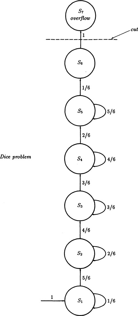
Suppose we have a situation, like the coin toss, good or defective component, life or death, etc. where there is only one of two possible outcomes. We also suppose that the trials are independent and of constant probability. We ask when the event occurs for the first time.

Example 4.2–1    First Occurrence

Let the probability of the event be p ≠ 0, and let X be the random variable that describes the first occurrence of the event. Then we have (repeating 4.4–1)

$\begin{array}{c}\mathrm{Pr}\{X=1\}=p\\ \mathrm{Pr}\{X=2\}=qp\\ \mathrm{Pr}\{X=3\}=q^{2}p\\ \cdots \\ \mathrm{Pr}\{X=k\}=q^{k-1}p\\ \cdots \end{array}$

These are the same probabilities as those of the sample space (4.1–1), and they form a geometric probability distribution.

Have we counted all the probability? We compute the infinite sum (via the usual calculus approach of first doing in our head the finite sum and then examining the result as the number of terms approaches infinity). We have the standard result (using 4.1–2)

${\displaystyle \sum }_{k=1}^{\infty }\mathrm{Pr}\{X=k\}={\displaystyle \sum }_{k=1}^{\infty }p{q}^{k-1}=\frac{p}{1-q}=\frac{p}{q}=1$

Thus the sample space has a total probability of 1 as it should.

This shows us how to get the generating function of the distribution. The variable t is a dummy variable having no real numerical value, but since we will later set it equal to 1 we must have the convergence of the infinite geometric progression for all q < 1 (at q = 1 the event cannot occur). The generating function is, therefore, from (4.1–2),

$G(t)={\displaystyle \sum _{k=1}^{\infty }p{q}^{k-1}{t}^k=\frac{pt}{1-qt}}$

(4.2–2)

To get the mean and variance we need the first two derivatives evaluated at t = 1, (see equations 2.7–3 and 2.7–4)

$G^{\prime }(t)=\frac{(1-qt)p-pt(-q)}{{(1-qt)}^2}=\frac{p}{{(1-qt)}^2}{G}^{\prime }(1)=p/p^2=1/p{G}^{″}(t)=\frac{2pq}{{(1-qt)}^3}{G}^{″}(1)=2q/p^2$

(4.2–2)

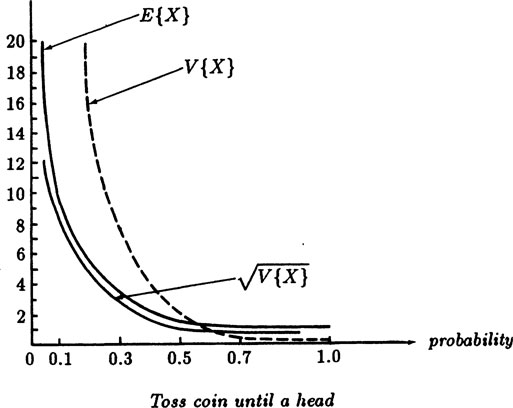
Hence the mean (expected time) is

$E\left\{X\right\}=1/p$

(4.2–3)*

In words, we have the important result that the expected value of a geometric distribution is exactly the reciprocal of the probability p. Since

$E\left\{X^2\right\}=G^{″}(1)+G^{\prime }(1)=2q/p^2+1/p$

FIGURE 4.2–1

the variance is, from 2.7–4,

$\begin{array}{ll}V\left\{X\right\}\hfill & =E\left\{X^2\right\}-E^2\left\{X\right\}=\frac{2q}{p^2}+\frac{1}{p}-{\left(\frac{1}{p}\right)}^2\hfill \\ \hfill & =\frac{2q+p-1}{p^2}=\frac{q}{p^2}\hfill \end{array}$

(4.2–4)*

If, as for a well balanced coin, p = 1/2 then the expected time to a head is two tosses, and the variance is also 2. In Figure (4.2–1) we plot as a function of p the mean, variance, and the square root of the variance, which is often used as a measure of what to expect as a reasonable deviation from the mean.

These results, (4.2–3) and (4.2–4), are important because they allow us to solve some problems very easily, as we will see in Examples (4.2–3) and (4.2–5).

Example 4.2–2    Monte Carlo Test of a Binomial Choice

There is much truth in the remark of Peirce (Section 2.1) that in human hands probability often gives wrong answers. We therefore twice simulated 100 trial runs on a programmable hand calculator and got the following table for the number of tosses until the first head.

TABLE 4.2–1
100 Simulations of coin tossing until the first head.

Run length	Frequency of run
No. of tosses	Theoretical	First run	Second run
1	50	53	52
2	25	24	27
3	12.5	13	10
4	6.25	8	5
5	3.125	1	3
6	1.5625	1	1
7	0.7813	0	1
8	0.3906	0	0
9	0.1953	0	0
10	0.0977	0	0
11	0.0488	0	0
12	0.0244	0	1

The computed E{X}, E {X²} and variance are:

	E{X}	E{X2}	V{X}
Theoretical:	2	6	4.00
Experiment #1:	1.83	4.55	3.03
Experiment #2:	1.895	6.34	4.64

We conclude that we are not wrong by the usual factor of 2, but must be fairly close. Either longer runs, or simulations for other than p = 1/2, would give further confidence in the results derived. In the first run the results were too bunched, and the large variance in the second experiment arose from the single outlier of a run of length 12. You have to expect that the unusual will occur with its required frequency if the theory reasonably models reality. The extreme of p = 1 gives E{X] = 1, V{X} = 0, while from Figure 4.2–1 the other extreme p = 0 gives infinity to both values, and these results agree with our intuition.

Example 4.2–3    All Six Faces of a Die

What is the expected number of rolls of a die until we will have seen all six faces (assuming, of course, a uniform distribution and independence of the rolls)?

Using the method of random variables we define:

X₁ = 1 the number of rolls until we see the first new face

X_i = the number of rolls after the (i − 1)st face until the i^th face, (i = 2,…, 6). Hence the random variable for the total number of rolls until we see all six is simply

$X=X_1+X_2+\cdots +X_6$

and the expected number is

$E\left\{X\right\}={\displaystyle \sum _{i=1}^{6}E\left\{X_i\right\}}$

But from the previous result, (4.2–3), the expected number is the reciprocal of the probability, and we have

$\begin{array}{cc}E\left\{X_i\right\}=1/\{(7-i)/6\}=6/(7-i)& (1=1,\dots 6)\end{array}$

Hence we have (recall the harmonic sums from Appendix 1.A)

$\begin{array}{c}E\left\{X\right\}=6\left\{\frac{1}{6}+\frac{1}{5}+\frac{1}{4}+\frac{1}{3}+\frac{1}{2}+1\right\}\\ =6H(6)=6\left(\frac{147}{60}\right)\\ =14.7\end{array}$

(4.2–4)

In other words, the expected number of rolls until you see all the faces is above 14 and less than 15.

One is inclined to interpret this expected value of 14.7 rolls to mean that the probabilty of success on 14 rolls is less than 1/2 and that for 15 it is greater than 1/2. To do this is to confuse the expected value with the median value—a common error! To see this point we give a simple example. Let the random variable X have

$P\{X=1\}=2/3$$P\{X=2\}=0$$P\{X=3\}=1/3$

Then the expected value of X is

$E\left\{X\right\}=1\left(\frac{2}{3}\right)+2(0)+3\left(\frac{1}{3}\right)=\frac{5}{3}$

Thus the expected number of trials is 5/3 but 2/3rds of the time you win on the first trial! Other examples are easily made up to show that the expected value and the median value can be quite different.

How about the variance? The random variables X_i were carefully chosen to be independent of each other, hence their variances add, and we have, from (4.2–4) and q_i = 1 – p_i,

$\text{Var}\left\{X\right\}={\displaystyle \sum _{i=1}^6\frac{q_i}{p_i^2}}={\displaystyle \sum _{i=1}^6\left[\frac{1}{p_i^2}-\frac{1}{p_i}\right]}$

The p_i = (7 – i)/6, and when you set k = 7 – i, (k = 1,…, 6), p_i = k/6 you have

$\begin{array}{c}\text{Var}\left\{X\right\}={\displaystyle \sum _{k=1}^6\left[\frac{36}{k^2}-\frac{6}{k}\right]}\\ =36[1+1/4+1/9+1/16+1/25+1/36]-14.7\\ =[36+9+4+9/4+36/25+1]-14.7\\ =53+69/100-14.7=38.99\end{array}$

(4.2–5)

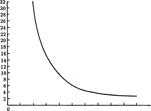
Thus the root mean square deviation from the expected value is 6.244…, and we therefore might expect a range for the trials running from 8.5 to 20.9, though, of course, we must expect to see many trials fall ouside these limits. The lowest possible number of trials is 6 which, from Example 3.2–1, has a probability of 6!/6⁶ = 0.015432… ~ 1½%

Example 4.2–4    Monte Carlo Estimate

To check both the particular case, and the model generally, we did a Monte Carlo simulation using 1000 trials. Part of the results are given in Table 4.2–2.

TABLE 4.2–2
Monte Carlo Until All Six Faces of a Die Appear.

Number of trials	Probability cumulated
n	p
⋮
10	0.272
11	0.356
12	0.438
13	0.514
14	0.583
15	0.644
16	0.698
17	0.745
18	0.785
19	0.819
20	0.848
∶

and we see that by linear interpolation for p = 1/2 we have 12.815 as the median number of trials. This is somewhat far from the average number 14.7 because the distribution is skewed a bit. It is important to stress that the median and average can be quite different—the median is the item in the middle and is relatively little affected by the tails of a distribution, while the average covers all the distribution and can be strongly affected by the tails.

Example 4.2–5    Card Collecting

Often packages which you buy in a store include a card with a picture, or other items of a set, and you try to collect all of the N possible cards. What is the expected number of trials you must make?

This is a simple generalization of the six faces of a die, (Example 4.2–3). The expected value is now

$\begin{array}{c}E\left\{X\right\}=N\left[\frac{1}{N}+\frac{1}{N-1}+\frac{1}{N-2}+\cdots +1\right]\\ =NH(N)\end{array}$

(4.2–6)

where $H(N)=1+1/2+1/3+\cdots +1/N~\mathit{ln\hspace{0.17em}}N$, the truncated harmonic series (see Appendix 1.A). The variance is correspondingly

$\text{Var}\left\{X\right\}=N^2{\displaystyle \sum _{k=1}^N\frac{1}{k^2}-{\left\{N{\displaystyle \sum _{k=1}^N\frac{1}{k}}\right\}}^2}$

These sums are easily bounded, as shown in Appendix 4.B, by

$\mathit{ln\hspace{0.17em}}N+\frac{N+1}{2N}\ge {\displaystyle \sum \frac{1}{k}\ge \mathit{ln\hspace{0.17em}}N+\frac{N+1}{2N}-\frac{(1-\frac{1}{N^2})}{8}}$$\frac{3}{2}-\frac{1}{N}+\frac{1}{2N^2}\ge {\displaystyle \sum \frac{1}{k^2}}\ge \frac{3}{2}-\frac{1}{N}+\frac{1}{2N^2}-\frac{(1-\frac{1}{N^3})}{4}$

so the general case is easily estimated. The differences between the bounds are the terms on the right extremes of the equations and dropping the 1/N² terms gives the values 1/8 and 1/4 respectively as the differences between the lower and upper bounds. Approximations may be closer many times.

Example 4.2–6    Invariance Principle of Geometric Distributions

The probability of not getting a head in n independent trials is qⁿ which we shall label as

$P(n)=q^n$

This is a geometric progression, and has the following property:

$\begin{array}{cc}P(n)=P(m)P(n-m)& \text{for all }m\text{ between }1\text{ and }n.\end{array}$

(4.2–7)

But this is the same, using conditional probabilities (Section 1.8), as

$P(n)=P(m)P(n-m|m)$

In words, we have that the probability of going n steps without the event happening is the same as the probability of going m < n steps multiplied by the probability of going n – m steps conditioned on having gone m steps. Thus, comparing the two equations we see that having gone m steps does not affect in any way the probability of continuing—that for the case of a geometric progression the past and future are disconnected. In different words, the probability of getting a head is independent of how many tails you have thrown—but that is exactly the concept of independence! There is an invariance in a geometric probability distribution—if you get this far without the event happening then the expected future is the same as it was before you started!

The converse is also true; if you have this property then the discrete sequence must be simply the powers of the probability of a single event as can be seen by going step by step.

Example 4.2–7    First and Second Failures

Suppose we have a Bernoulli two way outcome, the toss of a coin, the test of success or failure, of life or death, of good or bad component, with probability p of a failure (which is the event we are looking for), and hence q of success (not failing). The generating function for the first failure is given by (4.2–2)

$\begin{array}{cc}G(t)=\frac{pt}{(1-qt)}& G(1)=1\end{array}$$\begin{array}{cc}{G}^{\prime }(t)=\frac{p}{{(1-qt)}^2}& G^{\prime }(1)=\frac{1}{p}\end{array}$$\begin{array}{cc}{G}^{″}(t)=\frac{2pq}{{(1-qt)}^3}& G^{″}(1)=\frac{2q}{p^2}\end{array}$

with the corresponding mean 1/p and variance q/p², (4.2–3) and (4.2–4). The time to second failure will be just the convolution of this distribution with itself since the time to second failure is the sum of the time to the first plus the time to the second failure. For the second failure we have, therefore, the generating function

$\begin{array}{cc}H(t)=G^2(t)={\left[\frac{pt}{1-qt}\right]}^2& H(1)=1\end{array}$

The convolution clearly sums up exactly all the possibilities; the probability that the first failure occurred at each possible time in the interval and that the second occurred exactly at that point where the sum is the coefficient of t^k. By expanding (1 – qt)^-2 using (4.1–3) we can get the actual numbers, kpq^k–1.

To find the mean and variance of the distribution H(t) = G²(t) we have

$H^{\prime }(t)=2G(t)G^{\prime }(t)$

hence the mean time to second failure is, since G’(1) = 1/p

$H^{\prime }(1)=2(1)(1/p)=2/p=1/p+1/p$

as you would expect. For the second derivative we have, since G”(1) = 2q/p,

$H^{″}(t)=2G(t)G^{″}(t)+2{[G^{\prime }(t)]}^2$$H^{″}(1)=2(1)\left(\frac{2q}{p^2}\right)+2{\left(\frac{1}{p}\right)}^2=\frac{(4q+2)}{p^2}=\frac{6-4p}{p^2}$

hence the variance is

$\begin{array}{c}V=\frac{6-4p}{p^2}+\frac{2}{p}-\frac{4}{p^2}=\frac{6-4p+2p-4}{p^2}\\ =\frac{2-2p}{p^2}=\frac{2q}{p^2}\end{array}$

and we see again that for independent random variables the mean and variance add. For q = 0, p = 1, we have the mean = 2 and variance = 0 as it should. For p = 1/2 we get mean = 4 and variance = 4. See Figure 4.2–1.

Example 4.2–8    Number of Boys in a Family

Suppose there is a country in which married couples have children until they have a boy, and then they quit having more children. Suppose, also, that births are a Bernoulli process. What is the average fraction of boys in a family?

First, let p = the probability of a boy, hence q = 1 – p = the probability of a girl. We have

Size of family	Probability
1	p
2	qp
3	q2p
…	…
k	qk-1p
…	…

The average family size will be from (4.1–3)

${\displaystyle \sum _{k=1}^{\infty }k{q}^{k-1}p=\frac{p}{{(1-q)}^2}=\frac{1}{p}}$

The ratio of boys to the total population is, since it is a Bernoulli process, exactly p. But let us check this by direct computation. We have for the following expression, in the numerator the probability of a boy in the family for each size of family and in the denominator probability of there being the corresponding number of children in the family, each arranged by the size of the family,

$\frac{p+qp+q^{2}p+\cdots }{1+2qp+3q^{2}p+\cdots }=\frac{\frac{p}{1-q}}{\frac{p}{{(1-q)}^2}}=p$

We are now ready for the original question, what is the fraction of boys in the average family. We have

$(1)p+\frac{qp}{2}+\frac{q^{2}p}{3}+\cdots$$=p\left[1+\frac{q}{2}+\frac{q^2}{3}+\cdots \right]$

To sum the series in the square bracket we label it f(q). Then

$f(q)=1+\frac{q}{2}+\frac{q^2}{3}+\cdots$$qf(q)=q+\frac{q^2}{2}+\frac{q^3}{3}+\cdots$

Differentiate with respect to q

$\{qf(q){\}}^{\prime }=1+q+q^2+\cdots =\frac{1}{1-q}$

We integrate both sides. (Note that 0f(0) = 0 and that ln 1 = 0 so the constant of integration is 0.)

$qf(q)=-\mathit{ln\hspace{0.17em}}(1-q)=-\mathit{ln\hspace{0.17em}}p$

From this we get back to the original expression we wanted (4.2–9)

$-\frac{p}{q}\mathit{ln\hspace{0.17em}}p$

(4.2–10)

as the average fraction of boys in the family. For p = 1/2 we get

$\mathit{ln\hspace{0.17em}}2=0.693\dots ~0.7$

Thus half of all children are boys, but the fraction of boys in the average family is almost 7/10. The difference is, of course, that we are taking different averages.

As a check on the formula (4.2–10) we ask what value we get if p → 0, (boys are never born). The result is the fraction of boys approaches 0 in the families. If p → 1 (only boys are born) the formula approaches the value 1, just one child in each family, and again this is what you would expect. Hence the formula passes two reasonable checks, though at first sight the value for p = 1/2 seems peculiar.

Example 4.2–9    Probability that Event A Precedes Event B

If there are three kinds of events, A, B, and C with corresponding probabilites p(a), p(b), and p(c), what is the probability that event A will precede event B?

In the sample space of sequences of events the sequences

$\left\{C^{n-1}A\right\}$

will all be successes and only these. This probability is, (since p(a) + p(b) + p(c) = 1)

$\begin{array}{c}P(A)=p(a){\displaystyle \sum _0^{\infty }{p}^n(c)=\frac{p(a)}{1-p(c)}}\\ =\frac{p(a)}{p(a)+p(b)}\end{array}$

Similarly for the event B preceding A

$P(B)=\frac{p(b)}{p(a)+p(b)}$

Note that the answer does not depend on p(c) and that in practice event C can be the sum of many indifferent events (with respect to events A and B).

Example 4.2–10  Craps

The rules for the game of “craps” are that on the first throw of two dice:

You win on the sum 7 or 11

You lose on the sum 2, 3, or 12

Else this throw determines your “point.”

If you get a “point” you continue to throw the pair of dice until

You win if you throw your point

You lose if you throw a 7.

Using the notation p(i) = probability of the sum of the two dice being i, you win with probability (using the results of Example 4.2–9)

$P=p(7)+p(11)+{\displaystyle \sum _{i=4,5,6,8,9,10}p(i)\frac{p(i)}{p(i)+p(7)}}$

By symmetry

$\begin{array}{cc}p(2+j)=p(12-j)=\frac{(1+j)}{36},& i=0,\dots ,5\end{array}$

Hence

$P=p(7)+p(11)+2{\displaystyle \sum _{4,5,6}\frac{p^2(i)}{p(i)+p(7)}}$

Putting in the numbers we have

$\begin{array}{c}P=\frac{6}{36}+\frac{2}{36}+\frac{2}{36}\left\{\frac{3^2}{3+6}+\frac{4^2}{4+6}+\frac{5^2}{5+6}\right\}\\ =\frac{1}{18}\left\{3+1+\frac{9}{9}+\frac{16}{10}+\frac{25}{11}\right\}\\ =\frac{1}{18}\left\{5+\frac{8}{5}+\frac{25}{11}\right\}=\frac{1}{18}\left\{5+\frac{88+125}{55}\right\}\\ =\frac{1}{18}\left\{\frac{275+213}{55}\right\}=\frac{1}{18}\left\{\frac{488}{55}\right\}=\frac{1}{9}\left\{\frac{244}{55}\right\}\\ =0.492929\dots \end{array}$

Thus the game is slightly unfavorable to the person with the dice, and this explains why the “house” does not handle the dice.

Exercises 4.2

4.2–1 Find the exact coefficients for Example 4.2–7 by long division.

4.2–2 Estimate how long you can expect to go to get all of a set of 100 items.

4.2–3 Show that the time to third failure is the cube of the corresponding generating function. Extend to the time for the k^th failure.

4.2–4 Make a plot of (4.2–10) as a function of p. Discuss its meanings.

4.2–5 In the game of “odd man out” (the person who pays the bill) find the expected duration of play. Ans 4/3 tosses.

4.2–6 If n people play the game of odd man out what is the expected duration of play? Ans. 2^n-1/n.

4.2–7 If an urn has w white balls, r red balls, and bblack balls, and you draw repeatedly (with replacement) what is the probability of getting a white ball before a black ball?

4.2–8 With the roll of two dice what is the probability of getting a 7 before getting an 11? Ans. 3/4.

4.2–9 In drawing cards at random with replacement and shuffling before the next draw, what is the probability of getting a spade before a red card?

4.2–10 From an urn with r red balls, w white balls, and b black balls, what is the probability of drawing a white ball before a black ball?

4.2–11 In an urn with 1 black ball, 2 red balls, and w white balls, what is the probability of getting a white ball before the black ball? Ans. w/(w + 1).

4.2–12 If half the cars coming down a production line are white, one third are black, one sixth are green and one sixth are mixed, what is the probability that you will see a white car before a black car? Ans. 3/5.

4.3    On the Strategy to be Adopted

In view of Peirce’s remark (section 2.1) about the unreliability of probability computations, even in the hands of experts, we need to consider very carefully how we are to treat, with reasonable confidence, the topic of infinite sample spaces. We must do this because probability modeling and the corresponding computations enter into many important projects in science and engineering, as well as into medicine, economics and social planning. Furthermore, the field of probability has the property, barely alluded to by Peirce, that often our intuition cannot provide the usual checks on the reliability of the results that are used in all other fields of human activity.

Peirce identified a major weakness as the lack of uniform methods (and we have frequently been guilty of this); most probability books use various trick methods to get the answers. Furthermore, the modeling is often very remote from reality and leaves the user in great doubt as to the relevance of the results obtained. Whenever we can we need to adopt elementary, uniform, easy to understand methods, and to avoid “hi falutin,” “trick” or “cute” mathematics. But if we are to handle a wide class of problems we will need powerful mathematical methods. We assume the ability to handle the calculus, simple linear algebra, and ordinary differential equations. The theory of linear difference equations with constant coefficients, which closely parallels that for linear differential equations, is given briefly in Appendix 4.A. We will avoid many of the methods of advanced mathematics since they can at times give very peculiar results whose application to the real world are some times dubious and occasionally clearly not appropriate (see Section 4.8) [St].

It is apparently a fact of life that discrete problems are not as often solvable in a nice, closed form as are the corresponding continuous problems. An examination of the calculus, which is the main tool for the continuous case, shows the difference between the two fields; compare both differentiation and integration of the calculus with differencing and summation for the finite calculus. In differentiation just before the limit is taken there are usually many terms, and most of them vanish in the limit leaving a comparatively simple expression, but in the finite differences they do not vanish. For integration there are three main tools; (1) rearrangement, (2) integration by parts, and (3) change of variable. In the corresponding summation of infinite series, we have the first two but not the third—there can be only trivial changes of variable since we must preserve the equal spacing of the terms. And it is the third of these tools that is the most widely used in the calculus to do integrations. Thus we cannot hope to solve as wide a class of problems in closed form in the discrete mathematics as we can in the continuous. This is one of the reasons we will be driven to studying the topic of continuous probability distributions in Chapter 5.

If we cannot expect to get many of the solutions to our problems in a nice, useful form, what can we do? The path often taken in text books is to carefully select the problems to be solved, but this leaves much to be desired. We know from Section 2.7 that if we can get the generating function then at least we can get the mean and variance of the distribution by simple differentiation. Thus we will focus on first getting the generating function, Section 4.5, and then the complete solution, if ever, from it. The generating function contains the distribution itself, and often we can get the distribution if we will do enough work (Section 4.6). It is also true that from the generating function alone we can get many properties of the distribution beyond the moments if we do more calculation.

The method of state diagrams is increasingly used in diverse fields such as electrical engineering and computer science, and has proved to be very powerful. The state diagram, by its recursive nature, allows us to represent in a finite form the potentially infinite sample space of possible outcomes. Hence we will concentrate on this uniform method as our main tool (as Peirce recommended). We must also give many non-intuitive examples to build up your intuition. In Section 3.6 we solved recursive problems by implicitly using state diagrams using two states, success and failure, and giving the transition probabilities of going from one to the other on successive steps.

The finite state diagram method also has the interesting property that the paradoxes to be discussed in Section 4.8 cannot be represented as finite state diagrams since they require a potentially infinite storage device to represent the amount of money to be paid and furthermore violate the requirement that state diagrams we will use generally have constant transition probabilities.

4.4    State Diagrams

It is easier to show what state diagrams are by giving examples than it is to define them clearly. We begin with a simple problem, the distribution of the number of tosses of a coin until two heads appear in a row. We will proceed slowly, discussing why we do what we do at the various stages, and after this problem we will attack a slightly harder one which will indicate the general case.

FIGURE 4.4–1

This method of state diagrams and difference equations has been already used in the problems of Section 3.5 where we set up the transition probabilities from the various states and solved the corresponding difference equations with their boundary conditions. We now turn to further Examples.

Example 4.4–1    Two Heads in a Row

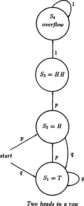
We begin with the state diagram. The states we need are S₁ (T, tail), S₂ (H, head), S₃ (HH, two heads in a row), and S₄ (the overflow state) The last is needed if we want to apply the conservation of probability rule so that the sum of all the probabilites is 1. See Figure 4.4–1 where each state is shown as well as the transition probabilities. It also allows the easy calculation of the expected value of some desired state.

It is well to work on a general case rather that the special case of p = 1/2 for H and T so that we can follow the details more clearly. It is a curious fact that often in mathematics the general case is easier to handle than is the special case! Therefore, we suppose that on the first toss the probability of H is p, and the probability of a T is q, shown in the figure on the left by arrows coming into the state diagram.

We now write the transition equations for the state S_i(n) in going from trial (n − 1) to trial n, (see Examples in Section 3.6 for similar equations). Let S_i(n) be the probability of being in state S_i at time n ≤ 2. Then for state S₁ (T, tails) we have

$S_1(n)=q{S}_1(n-1)+q{S}_2(n-1)$

For state S₂ (H, heads) we have

$S_2(n)=p{S}_1(n-1)$

For state S₃ (HH, two heads in a row) we have

$S_3(n)=p{S}_2(n-1)$

And for state S₄ (the overflow state) we have

$S_4(n)=S_3(n-1)+S_4(n-1)$

If we add all these equations we get

$S_1(n)+S_2(n)+S_3(n)+S_4(n)=(q+p)S_1(n-1)+(q+p)S_2(n-1)+S_3(n-1)+S_4(n-1)$

and we see that probability is conserved provided we use the overflow state S₄(n) which has no influence on the problem. We now drop the state S₄(n), though in a difficult problem we might include it to get a further consistency check on the results.

We now have a set of three difference equations,

$S_1(n)=q{S}_1(n-1)+q{S}_2(n-1)$$S_2(n)=p{S}_1(n-1)$$S_3(n)=p{S}_2(n-1)$

together with the initial conditions, $S_1(1)=q,S_2(1)=p,S_3(1)=0$. Note that the starting total probability is 1.

There are various methods for solving these equations. The first, and somewhat inelegant, method we will use to solve the equations 4.4–1 is to eliminate the states we are not interested in, S₁(n) and S₂ (n). When we eliminate S₂(n) (actually S₂(n − 1)) we get the equations

$S_1(n)=q{S}_1(n-1)+qp{S}_1(n-2)$$S_3(n)=p^2{S}_1(n-2)$

We next eliminate state S₁(n) by substituting the S₁(n) from the second equation (with the argument shifted by 2 and by 1) into the first,

$S_3(n+2)/p^2=(q/p^2)S_3(n+1)+(q/p)S_3(n)$

We easily see that the initial conditions for state S₃(3) are

$\begin{array}{cc}{S}_3(1)=0,& S_3(2)=p^2\end{array}$

Multiply the difference equation through by p² to get it in the standard form

$S_3(n+2)-q{S}_3(n+1)-pq{S}_3(n)=0,$$\begin{array}{cc}{S}_3(1)=0,& S_3(2)=p^2\end{array}$

(4.4–2)

To check this equation we try the two extreme cases, p = 0 which gives S₃(n) = 0 for all n, and the case p = 1 which gives q = 0 and S₃(n) = 1 for n = 2 and 0 otherwise.

Equation (4.4–2) is a homogeneous second order linear difference equation with constant coefficients, and according to Appendix 4.A it generally has eigenfunctions of the form rⁿ. Substituting rⁿ into the difference equation (4.4–2) and dividing out the rⁿ we get the characteristic equation

$r^2-qr-qp=0$

(4.4–3)

whose roots are

$r_1=(1/2)[q+\sqrt{q^2+4pq}]=(q+R)/2$$r_2=(1/2)[q+\sqrt{q^2+4pq}]=(q-R)/2$

(4.4–4)

where the quadratic irrationality is contained in

$R=\sqrt{q^2+4pq}$

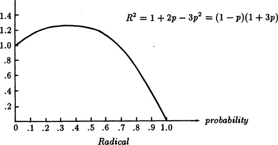
Note also the relationships, $r_1+r_2=q,r_1{r}_2=-pq,r_1-r_2=R$ which we will need later. How big is R, or rather R²? We set

$R^2=f(p)=q^2+4pq$$=1+2p-3p^2=(1-p)(1+3p)$

(4.4–5)

The maximum of the curve f(p) occurs at f′(p) = 0, namely at

$\begin{array}{cc}{f}^{\prime }(p)=2-6p=0,& \text{or }p=1/3.\end{array}$

At this maximum place

$f(1/3)=(1-1/3)(1+1)=4/3$

FIGURE 4.4–2

See Figure 4.4–2 for f(p) = R². We have R = 1 for both p = 0, and p = 2/3. Thus f(p) > 1 for 0 < p < 2/3.

Accordingly, we write the general solution of the difference equation (4.4–2) as (p ≠ 1)

$S_3(n)=C_1{r}_1^n+C_2{r}_2^n$

(4.4–6)

where C₁ and C₂ are constants to be determined by fitting the initial conditions S₃(1) = 0, S₃(2) = p². Thus we get

$S_3(1)=0=C_1{r}_1+C_2{r}_2$$S_3(2)=p^2=C_1{r}_1^2+C_2{r}_2^2$

To solve for C₂ multiply the top equation by r₁ and subtract the lower equation

$-p^2=C_2[r_2(r_1-r_2)]=C_2{r}_{2}R\Rightarrow C_2=-p^2/r_{2}R$

To solve for C₁ multiply the top equation by—r₂ and add to lower equation

$p^2=C_1[r_1(r_1-r_2)]=C_1{r}_{1}R\Rightarrow C_1=p^2/r_{1}R$

Hence the solution to the difference equation satisfying the initial conditions is

$\begin{array}{c}{S}_3(n)=\frac{p^2}{R}[r_1^{n-1}-r_2^{n-1}]\\ =\left(\frac{p^2}{R}\right)\left[{\left\{\frac{p+R}{2}\right\}}^{n-1}-{\left\{\frac{p-R}{2}\right\}}^{n-1}\right]\end{array}$

(4.4–7)

If we examine 4.4–7 closely, we see that the radical R will indeed cancel out and we will have a rational expression in p and q. We can check it for n = 1, and n = 2, and of course it fits the initial conditions since we chose the constants so that it would. If we use n = 3 we get

$S_3(3)=\left\{\frac{p^2}{r_1-r_2}\right\}[r_1^2-r_2^2]=p^2[r_1+r_2]=p^{2}q$

This is correct since to get a success in three steps you must have first a q and then two p’s.

To understand this formula in other ways let us rearrange it, remembering that r₁ – r₂ = R,

$S_3(n)=\left(\frac{p^2}{r_1-r_2}\right)r_1^{n-1}\left[1-{\left(\frac{r_2}{r_1}\right)}^{n-1}\right]$

hence as n gets large only the first part in the square brackets is left and S₃(n) approaches

$\left(\frac{p^2}{r_1-r_2}\right)r_1^{n-1}=\frac{p^2}{R}{r}_1^{n-1}$

(4.4–8)

The approach is surprisingly rapid when the roots are significantly different (R is not small).

The cancellation of the quadratic irrationality R in this problem is exactly the same as in the classic problem of the Fibonacci numbers which are defined by

$\begin{array}{ccc}{f}_{n+1}=f_n+f_{n-1},& \text{where}& f_0=0,f_1=1\end{array}$

The solution is well known to be (see Appendix 4.A)

$f_n=\frac{1}{\sqrt{5}}\left[{\left\{\frac{1+\sqrt{5}}{2}\right\}}^{n-1}-{\left\{\frac{1-\sqrt{5}}{2}\right\}}^{n-1}\right]$

(4.49)

and the radical $\sqrt{5}$ cancels out as it must since clearly the Fibonacci numbers are all integers.

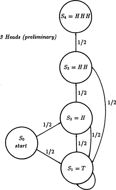
Example 4.4–2    Three Heads in a Row

The probability of tossing three heads in a row leads again to an infinite sample space. This time we use the states:

S0:	$\cancel{0}$
S1:	T
S2:	H
S3:	HH
S4:	HHH

FIGURE 4.4–3

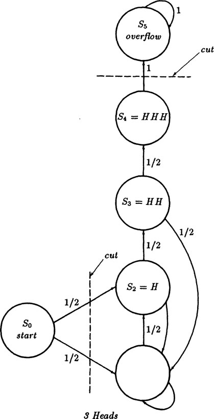
For a well balanced coin the probabilities of going from one state to another are as indicated in the graph of Figure 4.4–3. We see that out of every state the total probability of the paths is 1, except from state S₄. This fact comes close to a rule of conservation of probability. To make the rule inviolate (and conservation rules have proved to be extremely useful in physics and other fields) we again append a further state, S₅, Figure 4.4–4 from which state it goes to itself with probability 1. As before you can think of state S₅ as the overflow state that is needed to conserve probability. Thus we will have the powerful check at all stages that the total probability is 1.

FIGURE 4.4–4

Using the modified diagram with state S₅ included, Figure 4.4–4, we write the equations for the probability of being in state S_i at time n as S_i(n), i = 1,2,…, 5. We get for the states

$S_1(n)=(1/2)S_1(n-1)+(1/2)S_2(n-1)+(1/2)S_3(n-1)$$S_2(n)=(1/2)S_1(n-1)$$S_3(n)=(1/2)S_2(n-1)$$S_4(n)=(1/2)S_3(n-1)$$S_5(n)=S_4(n-1)+S_5(n-1)$

(4.4–10)

We notice that the equation for S₀(n) does not occur since there are no entry arrows, only exit arrows. We have, if you wish, S₀(0) = 1, and S₀(n) = 0 for n > 0, but this state has no use in the rest of the problem.

We check for the conservation of probability by adding all the equations.

$S_1(n)+S_2(n)+S_3(n)+S_4(n)+S_5(n)$$=S_1(n-1)+S_2(n-1)+S_3(n-1)+S_4(n-1)+S_5(n-1)$

Yes, the probability is conserved and the total probabilty is 1 since it checks for n = 0 (if we include S₀(0) = 1) and for n = 1 we have S₁(1) + S₂(1) = 1 with all other S_i = 0.

The conservation of probability allows us to think of the probability as an incompressible fluid, like water. The fluid flows around the system, and does not escape (provided we put in the overflow state, S₅ in this case); we look only at discrete times t = 0,1,2,…. The fluid analogy provides a basis for some intuition as to how the system will evolve and what is reasonable to expect; it provides us with a valuable check on our results.

Equations (4.4–10) are homogeneous linear difference equations with constant coefficients. For such equations the eigenfunctions (see Appendix 4.A) are simply

$r^n$

This time instead of eliminating all states except the desired one, as we did in Example 4.4–1, we will solve them as a system. Thus we assume the representation

$S_1(n)=A_1{r}^n$$S_2(n)=A_2{r}^n$$S_3(n)=A_3{r}^n$$S_4(n)=A_4{r}^n$$S_5(n)=A_5{r}^n$

where the A_i are constants and r will later be found to be a characteristic root. We get the system of homogeneous linear algebraic equations

$A_{1}r=(1/2)A_1+(1/2)A_2+(1/2)A_3$$A_{2}r=(1/2)A_1$$A_{3}r=\begin{array}{cc}& (1/2)A_2\end{array}$$A_{4}r=\begin{array}{ccc}& & (1/2)A_3\end{array}$$A_{5}r=\begin{array}{cccc}& & & A_4+A_5\end{array}$

Since we are interested in state S₄ we will apply an obvious rule that if we can “cut” a state diagram into two or more parts such that each part has only outgoing arrows that can never lead back, then for states within the part we will need to use only the eigenvalues that arise from those equations in the subset. The arrows entering the region provide the “forcing term” of the corresponding difference equations; the outgoing arrows have no further effects on the set of equations. We can therefore neglect them, for all other states; for example the state S₅ with its eigenvalue r = 1 and the state S₀ with its eigenvalue 0.

A standard theorem of linear algebra states that the homogeneous linear equations that remain can have a nontrivial solution if and only if the determinant of the system is 0. The determinant (after transposing terms to the left) is

$\left|\begin{array}{ccc}r-1/2& -1/2& -1/2\\ -1/2& r& 0\\ 0& -1/2& r\end{array}\right|=0$

(4.4–11)

The characteristic equation is, upon expanding the determinant,

$r^3-(1/2)r^2-(1/4)r-1/8=0$

(4.4–12)

We will label the three roots of the cubic r₁ = 0.9196…, r₂, r₃ = -0.2098 ± 0.3031i.

From the linearity of these equations we know that the probability of any of these states S_i can be written as a linear combination of powers of these three eigenvalues (characteristic roots). Since there are no multiple roots we have, therefore,

$S_4(n)=C_1{r}_1^n+C_2{r}_2^n+C_3{r}_3^n={\displaystyle \sum _{1=1}^3{C}_i{r}_i^n}$

(4.4–13)

The unknown coefficients C_i are determined by the initial conditions, but rather than finding them now we will find the generating function G(t) for the probabilities of the state of S₄(n). It is found by multiplying the nth of the equations (4.4–13) by tⁿ and summing

$G(t)={\displaystyle \sum S_4(n)t^n}={\displaystyle \sum _{i=1}^3{\displaystyle \sum _{n=1}^{\infty }{C}_i{(r_{i}t)}^n}}$

These are three infinite geometric progressions with the first term r_it and the common ratio r_it, hence they are each easily summed (see 4.2–1) to get

$G(t)={\displaystyle \sum _{i=1}^3{C}_i{r}_{i}t/(1-r_{i}t)}$$=t\left[\frac{C_1{r}_1}{1-r_{1}t}+\frac{C_2{r}_2}{1-r_{2}t}+\frac{C_3{r}_3}{1-r_{3}t}\right]$

(4.4–14)

The common denominator of these three terms is

$(1-r_{1}t)(1-r_{2}t)(1-r_{3}t)=D(t)$

(4.4–15)

This denominator resembles the original characteristic polynomial except that the coefficients are reversed. This reversal comes about because when you examine a typical factor in the form

$(1-r_{i}t)=t\left[\frac{1}{t}-r_i\right]$

you see the reversal, and hence in the product of all the factors you have tⁿ times the characteristic polynomial (4.4–12) in 1/t. This, in turn, means that you merely have the polynomial with the coefficients in reverse order!

In this method the characteristic equation begins with rⁿ with unit coefficient. But in general it might not be exactly the polynomial since the roots determine a polynomial only to within a multiplicative constant. Any scale factor that may be accidentally included in the denominator will be exactly compensated for when we find the numerator from the initial conditions so this delicate point is of no practical significance. Thus we have the denominator of the generating function

$D(t)=[1-(1/2)t-(1/4)t^2-(1/8)t^3]$

An examination of the numerator, excluding the front factor t, shows that it is of degree 2. Thus this numerator of the generating function must be of the form,

$N(t)=a_0+a_{1}t+a_2{t}^2$

FIGURE 4.4–5

where now

$G(t)=tN(t)/D(t)$

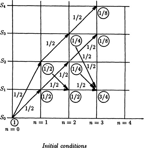
The coefficients a_i (i = 0, 1, 2) of the numerator are determined by the initial conditions, and hence we need three of them. Thus we evolve the state diagram for n = 1, 2, 3 as shown in Figure 4.4–5. The figure is easy to construct. To move from left to right we take the probability at each node, multiply it by the probability of going in each direction it can, and add all the contributions at the new node.

We are interested in state S₄(n) which has the initial conditions

$\begin{array}{cccc}{S}_4(0)=0,& S_4(1)=0,& S_4(2)=0,& S_4(3)=1/8\end{array}$

We have merely to divide the numerator of the generating function by the denominator to determine the unknown coefficients in the numerator. In this particular case we see immediately that the terms a₀ and a₁ are both zero and the next coefficient a₂ in N(t) is 1/8. The generating function is, therefore,

$G(t)=\frac{tN(t)}{D(t)}=\frac{\frac{t^3}{8}}{1-\frac{t}{2}-\frac{t^2}{4}-\frac{t^3}{8}}$

In this form of the solution we have neatly avoided all of the irrationalities and/or complex numbers that may arise in solving for the roots of the characteristic equation which in this case is a cubic.

You can see (using the water analogy) that all the probability in this problem will end up in the overflow state, hence it must all pass through the state S₄. This means, as you can easily check, that S₄(t) is a probability distribution and G(1) ≠ 1. Hence we can apply our usual methods. Had G(1) = 1, we could still handle the distribution as a conditional one, conditional on ending up in that overflow state, and this would require the modification of the method by dividing by the corresponding conditional probability.

To get the mean and variance we will need the first and second derivatives of N(t) and D(t) evaluated at t = 1. We have

$\begin{array}{cc}N(t)=t^2/8& N(1)=1/8\end{array}$$\begin{array}{cc}{N}^{\prime }(t)=2t/8& N^{\prime }(1)=2/8\end{array}$$\begin{array}{cc}{N}^{″}(t)=2/8& N^{″}(1)=2/8\end{array}$$\begin{array}{cc}D(t)=1-t/2-t^2/4-t^3/8& D(1)=1/8\end{array}$$\begin{array}{cc}{D}^{\prime }(t)=-1/2-t/2-3t^2/8& D^{\prime }(1)=-11/8\end{array}$$\begin{array}{cc}{D}^{″}(t)=-1/2-6t/8& D^{″}(1)=-10/8\end{array}$

We now have the pieces to compute the derivatives

$\begin{array}{c}{G}^{\prime }(1)=\frac{DN+Dt{N}^{\prime }-tN{D}^{\prime }}{D^2}\\ =\frac{\left(\frac{1}{8}\right)\left(\frac{1}{8}\right)+\left(\frac{1}{8}\right)\left(\frac{2}{8}\right)-\left(\frac{1}{8}\right)\left(\frac{-11}{8}\right)}{8^2}\\ =1+2+11=14\end{array}$

(4.4–16)

After some tedious work we have

$G^{″}(1)=324$

(4.4–17)

Hence the mean is 14 and the variance is

$\text{Var}=G^{″}(1)+G^{\prime }(1)-{[G^{\prime }(1)]}^2=142~{(12)}^2$

Notice that the generating function of each state S₁, S₂, S₃, or S₄, is determined by its own initial conditions since they are what determines the coefficients in the numerator; the denominator is always the same.

Exercises 4.4

4.4–1 Derive the solution of the Fibonacci numbers.

4.4–2 Solve Example 4.4–1 in the two extreme cases p = 1 and p = 0.

4.4–3 Repeat the Example 4.4–4 but now using the matrix method.

4.4–4 In Example 4.4–1 suppose you are to end on the state TH; find the mean and variance.

4.4–5 Do Example 4.4–2 except using the pattern HTH.

4.4–6 What is the generating function of the probability distribution of the number of rolls until you get two 6 faces in a row?

4.4–7 Find the generating function for the probability of drawing with replacement two spades on succesive draws.

4.4–8 What is the expected value and the variance for drawing (with replacement) two aces in a row from a deck of cards?

4.4–9 In Exercise 4.4–6 what is the mean and variance of the distribution?

4.5    Generating Functions of State Diagrams

We see that the essence of the method is to draw the finite state diagram, along with the constant probabilities of transition from one state to another. The method requires:

1. A finite number of states in the diagram (unless you are prepared to solve an infinite system of linear equations and act on the results).

2. The probabilities of leaving each state are constant and independent of the past (unless you can solve systems of difference equations with variable coefficients). Note that we have handled the apparent past history by creating states, such as the state HH, which incorporate some of the past history so that the state probabilities are independent of past history. Thus we can handle situations in which the probabilities at one stage can depend on a finite past history.

We will not be pedantic and state all the rules necessary for the use of the method on a particular state diagram, since the exceptions are both fairly obvious and seldom, if ever, arise in practice. When they do, the modifications are easy to make. They are also called Markov chains in some parts of the literature.

The steps in getting the rational generating function are:

1. Write the difference equations for each state and set up the matrix, and then the determinant

${(-1)}^n|A-rI|=|rI-A|=0$

This determinant gives the characteristic equation. Note that the subset you want can often be cut out of the entire state diagram, and if so then you probably need only consider the eigenvalues that come from that subset of the entire diagram. Generally you need to exclude overflow states since their total probability is not a probability distribution, and the corresponding generating function has infinity for its value at t = 1.

2. To find the generating function write the denominator as the characteristic polynomial with coefficients reversed, and assume unknown coefficients for the numerator. (It really does not matter how you scale the denominator, the numerator will adjust for it.) Note that t factors out of the numerator because you started with the first state n = 1.

3. Project forward (evolve) the probabilites of the variable you are interested in to get enough values to determine the unknown coefficients in the numerator N(t), and find them one by one. You then have the generating function

$G(t)=tN(t)/D(t)$

provided you start with the case n = 1.

4. Check that G(1) = 1. If it is not 1 then you have a conditional distribution (or else an error). If G(1) = 1 find G’(t) and G”(t) evaluated at t = 1, equations (4.4–6) and (4.4–7), and then get the mean and variance. (If these are only conditional distributions then you need to interpret them by dividing by their total conditional probabilities.)

5. If you want the detailed solution then the method of partial fractions is the next step, and is discussed in the next Section. If all you want is the asymptotic growth of the solution then this is easy to get since the solution is going to be dominated by the largest eigenvalue(s) (largest in absolute value). This can be seen when this root to the nth power is factored out of the solution, and the deviation from this dominating root easily estimated.

Example 4.5–1    The Six Faces of a Die Again

Example 4.4–2 solved the problem of the expected number of rolls of a single die until you have seen all six faces by what amounts to a trick method. Can we do it using state diagrams? To show that we can use the general method successfully (though it is true that often the effort is greater) we begin with the state diagram, Figure 4.5–1, with states S_i(i = 1,…, 6) where S_i means we have seen i distinct faces at that point. We get the equations

$S_1(n+1)=(1/6)S_1(n)$$S_2(n+1)=(5/6)S_1(n)+(2/6)S_2(n)$$S_3(n+1)=(4/6)S_2(n)+(3/6)S_3(n)$$S_4(n+1)=(3/6)S_3(n)+(4/6)S_4(n)$$S_5(n+1)=(2/6)S_4(n)+(5/6)S_5(n)$$S_6(n+1)=(1/6)S_5(n)$

These equations lead to the determinant for the characteristic roots

$\left|\begin{array}{cccccc}r-1/6& 0& 0& 0& 0& 0\\ -5/6& r-2/6& 0& 0& 0& 0\\ 0& -4/6& r-3/6& 0& 0& 0\\ 0& 0& -3/6& r-4/6& 0& 0\\ 0& 0& 0& -2/6& r-5/6& 0\\ 0& 0& 0& 0& -1/6& r\end{array}\right|=0$

This determinant nicely expands to the product

$(r-1/6)(r-2/6)(r-3/6)(r-4/6)(r-5/6)r=0$

The r = 0 root can be neglected so that the denominator becomes

$D(t)=(1-t/6)(1-2t/6)(1-3t/6)(1-4t/6)(1-5t/6)$

with D(1) = 5!/6⁵. What we want is S₆ (n) and we have

$\begin{array}{ccc}{S}_6(k)=0,& (k=1,\dots ,5)& S_6(6)=5!/6^5\end{array}$

Hence for the numerator we have

$\begin{array}{cc}tN(t)=5!t^6/6^5& N(1)=5!/6^5\end{array}$

FIGURE 4.5–1

We have, therefore,

$\begin{array}{cc}G(t)=tN(t)/D(t)& G(1)=1\end{array}$

We will need to calculate D’(1). To get it easily we first compute the logarithmic derivative

$\begin{array}{c}{D}^{\prime }(t)/D(t)={\displaystyle \sum _{k=1}^5(-k/6)/(1-kt/6)}\\ ={\displaystyle \sum _{k=1}^5\left[\frac{(-k)}{6-kt}\right]}\end{array}$

Therefore, by substituting the values we just calculated where they occur in the derivatives we have

$\begin{array}{c}{G}^{\prime }(1)=\frac{D(tN{)}^{\prime }-tN{D}^{\prime }}{D^2}\\ =\frac{5!}{6^5}\left\{\frac{\frac{5!}{6^5}(6)-\frac{5!}{6^5}{\displaystyle \sum \frac{(-k)}{6-k}}}{{\left(\frac{5!}{6^5}\right)}^2}\right\}\\ =6+\left[\frac{1}{5}+\frac{2}{4}+\frac{3}{3}+\frac{4}{2}+\frac{5}{1}\right]\\ =6+\frac{1}{5}+\frac{1}{2}+1+2+5=14+\frac{2+5}{10}\\ =14.7\end{array}$

which is the same answer but at a much more labor.

One has to ask the value of a trick method that gets the answer if you see the trick, vs. a general method that often involves a lot of work before you get the answer. Uniform methods as well as trick methods have their place in the arsenal of tools for solving problems, but there is probably more safety in the uniform methods (Peirce) and are more easily programmed on a computer that can take care of the messy details. Indeed, one could easily write a complete computer program to do such problems.

Exercises 4.5

4.5–1 Work the die problem if there are only three equally likely faces on the die.

4.5–2 Find the generating function for the distribution of getting three heads in a row while tossing a coin.

4.5–3 Compute the variance of the Example 4.5–1. 4.5–4 In Example 4.4–2 one sees that the generating function has the denominator (4.4–15) and that the partial fraction expansion is merely backing you up to (4.4–14), and thus the expansion in powers of t gets you to (4.4–13). Discuss the implications.

4.5–5 For Example 4.4–1 give the corresponding equations (4.4–7) and the actual terms.

4.5–6 Find the generating function (using the direct method) for getting three spades in a row from a deck of shuffled cards.

4.6    Expanding a Rational Generating Function

If you can factor the denominator into real linear and real quadratic factors (this can be done theoretically since any polynomial with real coefficients is the product of real linear and real quadratic factors, and by a computer in practice if necessary) you apply the standard method of partial fractions (remember to factor t out of the numerator before you start so that the degree of the numerator is less than that of the denominator as is required in partial fraction methods). You then divide out each factor to get it in the form of a sum of powers of t. Grouping the equal powers together you have the detailed values of the variable you are interested in.

In more detail, since the steps to do after the method of partial fractions is applied are often not discussed carefully:

(1) For a simple linear factor you have

$1/(1-rt)={\displaystyle \sum _{i=0}^{\infty }{r}^n{t}^n}$

(2) For repeated factors the derivatives of this expression with respect to r will produce the needed expansions.

(3) For a simple real quadratic x² – px + q with complex roots we have p² − 4q < 0. We use the complex polar form for the roots

$\begin{array}{c}1-pt+q{t}^2=(1-A{e}^{ix}t)(1-A{e}^{-ix}t)\\ =1-(2A\cos x)t+A^2{t}^2\end{array}$

which shows that $A=\sqrt{q}$ and, of course, p = 2A cos x which determines a real x (since p² < 4q). You now expand into partial fractions using unknown coefficients d₁ and d₂,

$\frac{1}{(1-A{e}^{ix}t)(1-A{e}^{-ix}t)}=\frac{d_1}{1-A{e}^{ixt}}+\frac{d_2}{1-A{e}^{-ixt}}$

After a little algebra

$\begin{array}{cc}{d}_1=\frac{e^{ix}}{2i\sin x}& d_2=\frac{-e^{-ix}}{2i\sin x}\end{array}$

hence

$\frac{1}{1-pt+q{t}^2}=\frac{e^{ix}}{2i\sin x}{\displaystyle \sum _{k=0}^{\infty }{A}^k{e}^{ikx}{t}^k-\frac{(e^{-ix})}{(2i\sin x)}}{\displaystyle \sum _{k=0}^{\infty }{A}^k{e}^{-ix}{t}^k}$$={\displaystyle \sum _{k=0}^{\infty }{A}^k\left\{\frac{e^{i(k+1)x}-e^{-i(k+1)x}}{2i\sin x}\right\}}$$={\displaystyle \sum _{k=0}^{\infty }{A}^k{t}^k\frac{\sin (k+1)x}{\sin x}}$

(4) For repeated quadratic factors, you differentiate this expression with respect to the parameter p to get the next higher power in the denominator, and of course make the corresponding adjustments in the numerator. To get rid of a factor of t in the numerator we have only to divide the expansion by t. With this you can add the proper combination (with and without t) to get the appropriate linear term, thus getting as a result two terms where you had one. Finally, you group the terms from the expansions for each power of t to get the coefficients of the generating function, and hence the probabilities of the state you are solving for. But remember the initial removal of the front factor of t. As before, it is the largest root in absolute value that dominates the solution for large n (or the set if there are more than 1 of that size).

To summarize, if we have the generating function we can get the mean and variance (and higher moments) by differentiation and evaluation at t = 1. If we want the general term of the solution then there seems to be no way other than to factor the denominator of the generating function (get the characteristic roots), and then carry out the partial fraction expansion and subsequent representation in powers of t. The coefficients of the powers of t are, from the definition of the generating function, the desired probabilities. Simple and repeated real linear and real quadratic factors can be handled in a regular fashion. But note that the algebraic (irrational) nature of the roots must cancel out in the end because the final answer is rational in the coefficients of the difference equations and the initial conditions. The well known example (discussed earlier) of this is the Fibonacci numbers (integers). However, if all we want are a few of the early coefficients then we can simply divide out the rational fraction to get the coefficients of the powers of t.

4.7    Checking the Solution

How can we further check the solution we have obtained? One way is to compute a few more values from the state diagram and compare them with those calculated from the solution. Another way of checking the solution is to generalize, or embed, the problem in a family of problems. This is often effective because the corresponding general solution contains the particular solution and may contain other, degenerate, solutions which are likely to be known to you so you can check the accuracy of the model and solution.

Example 4.7–1    Three Heads in a Row

Suppose we take the above problem (Example 4.4–2) except that the probability of a success is now p, and the complementary probability of failure is q = 1 – p. If p = 1 we know the solution, and if p = 0 we will again know the solution. If we further plot both the mean and variance as a function of p we will get a feeling for the problem and why we have, or have not, the correct result.

We merely sketch in the steps, leaving the details for the student. The characteristic equation will be

$r^3-q{r}^2-pqr-p^{2}q=0$

The corresponding generating function is (using the initial conditions)

$G(t)=t\left[\frac{p^3{t}^2}{1-qt-pq{t}^2-p^{2}q{t}^3}\right]$

We again adopt the notation

$G(t)=tN(t)/D(t)$$G^{\prime }(t)=[D(tN{)}^{\prime }-tN{D}^{\prime }]/D^2$$G^{″}(t)=[D(tN{)}^{″}-tN{D}^{″}]/D^2-2D^{\prime }{G}^{\prime }/D$

We have for the parts evaluated at t = 1

$\begin{array}{ccc}tN=p^3,& (tN{)}^{\prime }=3p^3,& (tN{)}^{″}=6p^3\end{array}$$\begin{array}{ccc}D=p^3,& D^{\prime }=3p^3-p^2-p-1,& D^{″}=6^3-4p^2-2p\end{array}$$\begin{array}{cc}{G}^{\prime }(1)=[1+p+p^2]/p^3,& G^{″}(1)=(\text{evaluate the parts above)}\end{array}$

At p = 1/2 this agrees with the previous results. Next we plot the values as a function of p as shown in Figure 4.7–1. If p = 0 then we will never get three successes in a row, while if p = 1 it will happen on the third trial and the corresponding variance will be zero. The curve confirms this.

FIGURE 4.7–1

4.8    Paradoxes

The simple, countably discrete sample space we have carefully developed can give some peculiar results in practice. The classic example is the St. Petersburg paradox. To dramatize the trouble with this paradox we follow it with the Castle Point paradox. We then turn to various “explanations” of the paradoxes—there are, of course, those who feel that they need no “explanation.” See also [St].

Example 4.8–1    The St. Petersburg Paradox

In this paradox you play a game; you toss a fair coin until you get a head, and the toss on which you first get the head is called the k^th toss. When the first success occurs on the k^th toss you are to be paid the amount

$2^k$

units of money and the game is over. How much should you pay to play this game, supposing you are willing to play a “fair game”?

The probability of a success on the k^th toss is exactly

$2^{-k}$

so the expectation on the k^th toss is exactly 1. Thus the sum of all the expectations is the sum of 1 taken infinitely many times! You should be willing to pay an infinite amount, or at least an arbitrarily large amount, to play.

When you think about the matter closely, and think of your feelings as you play, you will see that you would probably not be willing to play that sort of a game. For example, if you bet 128 units you will be ahead only if the first six faces are all tails—one chance in 128. Hence the question arises, “What is wrong?” You might want to appeal to the Bernoulli evaluation criterion, Sections 3.7 and 3.8, to get out of the difficulty.

Example 4.8–2    The Castle Point Paradox

To define this game we may take any sequence u(n) of integers approaching infinity no matter how rapidly. For example, we may use any of the following sequences,

$\begin{array}{cccc}u(n)=n& u(n)=n!& \text{or}& u(n)={(n!)}^{n!}\end{array}$

We will pick the third for purposes of illustration. These u(n) will be called “the lucky numbers.” If the first head in the sequences of tosses of a fair coin occurs on a lucky number you are paid, otherwise you lose. The payment is

$\frac{2^{u(n)}}{n}$

and again the probability of success on this toss is

$2^{-u(n)}$

This time the expectation on the n^th lucky number is 1/n. But the series

${\displaystyle \sum _{n=1}^{\infty }\frac{1}{n}}$

diverges to infinity, hence the total expectation is infinite.

Let us look at this game more closely. We have the table of the first 5 lucky numbers:

n	n!	(n!)n!
1	1	1
2	2	4
3	6	4.6656 × 104
4	24	1.3337 × 1033
5	120	3.1750 × 10249

There are less than 5 × 10¹⁷ seconds in 15 billion years (the currently estimated age of the universe). There are about 3.14 × 10⁹ seconds in 100 years so that if you tossed the coin once every microsecond (10^-6) you would do less than

$3.14\times {10}^{15}$

tosses in your lifetime, and you would not even reach the fourth lucky number. To reach the third lucky number you need 46,655 tails followed by 1 head! I could, of course, redefine the game so that the first three lucky numbers did not count, and still have the infinite series diverge to infinity and hence still have the paradox that to play the game you should be willing to pay an arbitrary amount of money.

Example 4.8–3    Urn with Black and White Balls

An urn contains 1 black and 1 white ball. On each drawing:

If ball is white then end of game

If ball is black return and add another black ball

Find the expected number of draws until you get a white ball.

The sample space of successes is

$\left\{b^{n-1}w\right\}$

and the total probability is

$\begin{array}{c}P=\frac{1}{2}+\frac{1}{2}\left(\frac{1}{3}\right)+\frac{1}{3}\left(\frac{1}{4}\right)+\cdots +\frac{1}{k}\left(\frac{1}{k+1}\right)+\cdots \\ =1-\frac{1}{2}+\frac{1}{2}-\frac{1}{3}+\frac{1}{3}-\frac{1}{4}+\cdots +\frac{1}{k}-\left(\frac{1}{k+1}\right)+\cdots \\ =1\end{array}$

hence we have the total probability of getting a white ball is 1. The expected number of draws is

$E\left\{K\right\}={\displaystyle \sum _{k=0}^{\infty }(k)\frac{1}{k(k+1)}}={\displaystyle \sum _{k=0}^{\infty }\frac{1}{k+1}}$

which is the harmonic series and diverges to infinity. Hence the expected number of draws until a white ball is drawn is infinite.

Given these paradoxes some people deny that there is anything to be “explained.” Hence for them there is nothing more to say.

There is, among other explanations, one which I will call “the mathematician’s explanation” (meaning you have to believe in this standard kind of mathematics). The argument goes as follows: since clearly it is assumed that you have an infinite amount of money, then to enter the game the first time you simply pay me every other unit of money you have, thus both paying me the infinite entry fee and also retaining an infinite amount for the next game. On my side, I similarly pay off for finite amounts and retain an infinite amount of money. Hence after many games we both retain an infinite amount of money and the game is “fair”!

An alternate explanation uses the standard “calculus approach”; assume finite amounts and see what happens as you go towards infinity. Assume in the St. Petersburg paradox that I have a finite amount of money, say A = 2ⁿ. Thus you can play at most n tosses and still be paid properly. At this point the expectation is

${\displaystyle \sum _{i=1}^{n}1=n={\log }_{2}A}$

and this is the log (base 2) of the amount of money I have. This seems to be more reasonable. If the maximum you could win is, say, 2²⁰ (approximately a million units) then risking 20 units is not so paradoxical. A similar analysis will apply to the Castle Point paradox. If you assume that only the first three lucky numbers are going to pay off then your expectation is

$1+1/2+1/3=11/6<2$

This seems, again, to be a reasonable amount to risk for the three possible payments (one of them is hardly possible). For the first two lucky numbers the expectation is 3/2.

The confusion arises when n goes to infinity and hence both your payment and the possible winnings, A and log₂ A in the St. Petersburg paradox, both go to infinity. The two very distinct quantities, A and log₂A, both approaching infinity, are being viewed in the limit as being the same.

There are other ways of explaining the paradoxes, including either redefining the game or else using what seem to be rather artificial definitions of what a fair game is to be. We will ignore such devices.

The purpose of these paradoxes is to warn you that the careless use of even a simple countably infinite discrete probability space can give answers that you would not be willing to act on in real life. Even in this discrete model you need to stop and think of the relationship between your probability model and reality, between formal mathematics and common experience. Note again that both the St. Petersburg and Castle Point paradoxes are excluded if you adopt the finite state diagram (with constant transition probabilities) approach, [St].

Most people assume, without thinking about it, that the mathematics which was developed in the past is automatically appropriate for all new applications. Yet experience since the Middle Ages has repeatedly shown that new applications often require modifications to the classically taught mathematics. Probability is no exception; probability arose long after the formation of the classical mathematics and it is not obvious that we should try to use the unmodified mathematics in all applications. We need to examine our beliefs, and the appropriateness of the usual mathematical model, before we adopt it completely. It may well be that the usual models of probability need various modifications of mathematics.

Exercises 4.8

4.8–1 Apply the Bernoulli value to the St. Petersburg paradox.

4.8–2 Find the generating function of Example 4.8–3.

4.8–3 Do a computer simulation of Example 4.8–3.

4.9    Summary

In this Chapter we have examined the simplest infinite sample spaces which seem to arise naturally. We found that there is a uniform method which is based on the finite state diagram representation of the problem. This method leads to rational generating functions, from which you can easily get both the mean and the variance of the distribution.

If you can factor the characteristic polynomial then you can get, via partial fractions and dividing the individual terms out, the actual terms of the generating functions in terms of sums of powers of the characteristic roots. But the values of the solution are rational in the coefficients and initial conditions, while generally speaking the characteristic roots are algebraic! It follows that the algebraic part of the solution must in fact cancel out, that somehow the sums of the roots that occur must be expressible in terms of the coefficients of the characteristic equation and products of the transition probabilties, namely by simply dividing out the rational fraction.

We introduced the safety device of the conservation of probability; it involves one extra state (which you generally do not care about though it may be needed in some problems). It also provides an intuitive way of thinking about problems as if probability were flowing water.

We also warned you that even this simple model can give some startling results if you try to apply standard mathematics without careful thinking; the Castle Point paradox was designed to dramatize the effect. The finite state diagram provides some safety in these matters.

Appendix 4.A Linear Difference Equations

Linear difference equations with constant coefficients are treated almost exactly the same way as are linear differential equations with constant coefficients (because of the common underlying linearity). Therefore we first review the theory of linear differential equations with constant coefficients.

For the linear differential equation with constant (real) coefficients (where yⁿ) means the n^th derivative of y)

$a_0{y}^{(n)}(x)+a_1{y}^{(n-1)}(x)+\cdots +a_{n}y(x)=f(x)$

(4.A–1)

the knowledge of any particular integral of (4.A–1), call it Y (x), reduces the problem to the homogeneous equation

$a_0{y}^{(n)}(x)+a_1{y}^{(n-1)}(x)+\cdots +a_{n}y(x)=0$

(4.A–2)

The eigenfunctions of this homogeneous equation are essentially the exponentials (“essentially” because of the possibility of multiple roots in the characteristic equation)

$y(x)=e^{mx}=\exp (mx)$

When this function is substituted into (4.A–2) we get the characteristic equation, since the exponential cancels out (as it must since we used eigenfunctions),

$a_0{m}^n+a_1{m}^{n-1}+\cdots +a_n=0$

(4.A–3)

This equation has the n characteristic roots

$\begin{array}{ccccc}{m}_1,& m_2,& m_3,& \dots ,& m_n\end{array}$

If all the characteristic roots are distinct then the general solution of the homogeneous equation is

$y(x)={\displaystyle \sum _{k=1}^n{C}_k{e}^{m_{k}x}}$

(4.A–4)

For a double root you try both x exp(mx) and exp(mx), for triple roots x²exp(mx), x exp(mx) and exp(mx), etc. If a root is complex then since we are assuming that the coefficients of the original differential equation are real the conjugate root also occurs. Let the roots be

$\begin{array}{ccc}a+ib& \text{and}& a-ib\end{array}$

In place of the two complex exponentials you can, if you wish, use instead

$e^{ax}\{C_1\cos bx+C_2\sin bx\}$

(4.A–5)

and multiple roots are treated just as in the case of simple roots (extra factors of x as needed). If we add the particular integral we assumed that we knew, Y(x), to the general solution of the homogeneous equation then we have the complete solution of the original equation (4.A–1).

For the linear difference equation

$a_{0}y(n+m)+a_{1}y(n+m-1)+\cdots +a_{n}y(n)=f(n)$

(4.A–6)

we again assume that we have a solution (integral) Y(n) of the complete equation and we are then reduced, as before, to the homogeneous equation

$a_{0}y(n+m)+a_{1}y(n+m-1)\cdots +a_{n}y(n)=0$

(4.A–7)

In place of the eigenfunctions exp(mx) we conventionally write (x becomes n of course)

$\begin{array}{ccc}{e}^{mn}=r^n& \text{and}& r=e^m\end{array}$

(4.A–8)

and we get the characteristic equation

$a_0{r}^n+a_1{r}^{n-1}+\cdots +a_n=0$

(4.A–9)

The general solution of the homogeneous equation is then of the form

$y(n)={\displaystyle \sum _{k=1}^n{C}_k{r}_k^n}$

(4.A–10)

and the rest is the same as for differential equations with the slight difference that multiple roots lead to

$\begin{array}{ccc}{r}^n,& n{r}^n,& n^2{r}^n,\dots \end{array}$

To illustrate the solution of a linear difference equation with constant coefficients we choose the perhaps best known example, that of the Fibonacci numbers which are defined by

$\begin{array}{ccc}{f}_{n+1}=f_n+f_{n-1},& f(0)=0,& f(1)=1\end{array}$

Each Fibonacci number is the sum of the previous two numbers.

Set f_n = rⁿ and we are led to the characteristic equation

$r^2-r-1=0$

whose solutions are

$\begin{array}{cc}{r}_1=\frac{1+\sqrt{5}}{2},& r_2=\frac{1-\sqrt{5}}{2}\end{array}$

Therefore the general solution is

$f_n=C_1{r}_1^n+C_2{r}_2^n$

Using the initial conditions we get the two equations

$f_0=0=C_1+C_2$$f_1=1=C_1{r}_1+C_2{r}_2$

Solving for these unknown coefficients C_i we get, after a little algebra,

$f_n=\frac{1}{\sqrt{5}}\left[{\left(\frac{1+\sqrt{5}}{2}\right)}^{n-1}-{\left(\frac{1-\sqrt{5}}{2}\right)}^{n-1}\right]$

Upon examinating how $\sqrt{5}$ enters into the square brackets we see, on expanding the binomials, that only the odd powers remain and that the front radical removes all quadratic irrationalities, as it must since from the definition all the Fibonacci numbers must be integers.

For the nonhomogeneous equation the particular integral of the original equation, Y(x) or Y(n) in the two cases, is usually found by plain, simple guessing at the general form, substituting into the equation, and finally determining the unknown coefficients of the assumed form using the linear independence of the terms to justify the equating of the coefficients of like powers of t.