5

Continuous Sample Spaces

5.1    A Philosophy of the Real Number System

It is natural to ask some one to pick an equally likely random point on the unit line segment. By the symmetry that most people perceive, or because nothing else was said, we see that the probability of picking any point must be the same as that of any other point. If we do not assign this value to be p = 0 then the total probability would be infinite. But apparently picking the probability to be zero for each point would lead to a zero total probability. Thus we are led to examine the usual mathematical answer that the real line is composed of points, having no length, but also that the unit line segment has length 1.

Indeed, up to now we have evaded, even in the infinite discrete probability space, a number of difficulties. For example you cannot pick a random (uniform) positive integer, because whatever number you name, “almost all” positive integers (meaning more than any fraction less than 1 you care to name) will be greater than the one you picked! If we choose to pick the positive integer n with corresponding probability

$p(n)=6/{(\pi n)}^2$

then the probability would total 1 (since $\Sigma 1/n^2={\pi }^2/6$). By and large in the previous chapter we dealt only with naturally ordered infinite sequences of probabilities; we did not venture into situations where there was no natural ordering. Thus we did not assign a probability distribution over all the rational numbers between 0 and 1. It can be done, but the solution is so artificial as to leave doubt in one’s mind as to the wisdom of its use in practice.

We have again raised the question of the relevance for probability theory of the usual real number system that was developed long before probability theory was seriously considered as a field of research. The real number system is usually developed from the integers (“God made the integers, the rest is man’s handiwork.” Kronecker), first by the extension to the rational numbers, and then by the extension to all real numbers via the assumption that any (Cauchy) convergent sequence of numbers must have a number as the limit. In the late middle ages the progress of physics found that the real numbers did not serve to describe forces, and the concept of vectors was introduced. Later the concept of a tensor was needed to cope with naturally occuring physical concepts. Thus without further examination it is not completely evident that the classical real number system will prove to be appropriate to the needs of probability. Perhaps the real number system is: (1) not rich enough—see non-standard analysis; (2) just what we want—see standard mathematics; or (3) more than is needed—see constructive mathematics, and computable numbers (below).

In the theory of computation, the concept of a computable number has proved to be very useful. Loosely speaking, a computable number is one for which a definite algorithm (process) can be given for computing it, digit by digit. The computable numbers include all the familiar numbers, including e, π, and γ. If by “describe” is meant that you can say how one can compute it digit by digit, then the computable numbers include all the numbers you can ever hope to describe. The set of computable numbers is countable because every computable number can be computed by a program and the set of programs is countable (programs are merely finite sequences of Os and Is).

What are all these uncountably many noncomputable numbers that the conventional real number system includes? They are the numbers which arise because it is assumed that “the limit of any Cauchy convergent sequence has a limiting number”; if you say, “the limit of any convergent sequence of describable numbers has a limit” then none of these noncomputable (uncountably many) numbers can arise. As an example of the consequences of what is usually assumed, take all the real numbers between 0 and 1 in the standard real number system, and remove the computable numbers. What is left is a noncountable set, no member of which you can either name or give an algorithm to compute it! You can never be asked to produce one of them since the particular number asked for cannot be described! Indeed, if you remove the computable numbers from each (half-open) interval (set) [k, k + 1), then according to the usual axiom of choice you can form a new set by selecting one number from each of these sets (whose members you can never describe!) and form a new set. How practical is this set? Is this kind of mathematics to be the basis of important decisions that affect our lives?

The intuitionists, of whom you seldom hear about in the process of getting a classical mathematical education, have long been articulate about the troubles that arise in the standard mathematics, including the paradoxes, in the usual foundations of mathematics. One such is the Skolem-Lohenheim paradox which asserts that any finite number of postulates has a realization that is countable. This means that no finite number of postulates can uniquely characterize the accepted real number system. When we apply the Skolem-Lohenheim paradox to the real number system we observe that (usually) the number of postulates of the real number system is finite hence (apparently) any deduction from these alone must not be able to prove that the set is noncountable (since any deduction from them alone must apply to all realizations of the model)! Again, the Banach-Tarski paradox, that a sphere can be decomposed into a finite number of congruent parts and reassembled to be a complete sphere of any other radius you choose, a pea size or the size of the known universe, suggests that we must be wary of using such kinds of mathematics in many real world applications including probability theory. These statements warn us that we should not use the classical real number system without carefully thinking whether or not it is appropriate for new applications to probability.

We should also note that isolated finite values of functions are traditionally ignored; thus

$\begin{array}{ccc}{\displaystyle \int f(x)dx}& \text{with}& |f(x)|\le M\end{array}$

over the intervals (a < x < b) and (a < x < b) have the same value. The isolated end values do not affect the result; indeed any finite number of (finite) missing values, or discontinuities, cannot affect the result (where we, of course, are assuming reasonable functions). The Riemann integral generally handles all the reasonable functions one can expect to meet when dealing with reality.

What are we to think of this situation? What is the role in probability theory for these numbers which can never occur in practice? Do we want to take over the usual real number system, with all its known confusions, when we have enough of our own? On the other hand, the real number system has the advantage that it is well known, (even its troubles are familiar), fairly well explored, and has comparatively few paradoxes left. As we go on and find further paradoxes in our probability work we need to ask whether the trouble arises from the nature of the assumed real number system or from the peculiar nature of the probability theory. See Section 8.5 for much the same argument.

5.2    Some First Examples

Rather than begin with some assumptions (postulates if you prefer) whose source, purposes, and reasonableness are not clear, we will begin by doing a couple of problems in a naive way so that you will see why probability theory has to make certain assumptions.

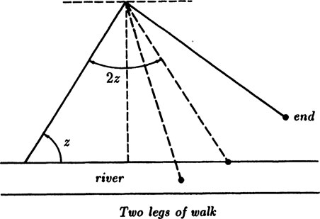
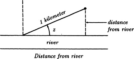
Example 5.2–1    Distance From a River

Suppose you are on the bank of a straight river and walk a kilometer in a randomly chosen direction. How far from the river will you be? Figure 5.2–1.

FIGURE 5.2–1

By implication we are restricted to directions away from the river, and hence angles z between 0 and π. By symmetry we see that we can restrict ourselves to angles between 0 and π/2, see Figure 5.2–1. It is natural to assume that all angles in the interval are equally likely to be chosen (because nothing else was said). If the angle is chosen to be z then we next have to think about the integral (rather than the sum) of all angles, and since the total probability must be 1 we have to normalize things so that the probability of choosing an angle in an interval Δz is

$(2/\pi )\Delta z.$

hence the total probability will be

${\displaystyle {\int }_0^{\pi /2}(2/\pi )dz=1}$

as it should.

Now to get the expected distance from the river we note that for the angle z the final distance is sin z (where z is the angle between the direction and the river). Hence the expected distance is the expectation of the variable sin z,

$\begin{array}{c}E\left\{\sin z\right\}={\displaystyle {\int }_0^{\pi /2}(2/\pi )\sin zdz}\\ =(2/\pi )(-\cos z)|{}_0^{\pi /2}=2/\pi =0.6366\dots \end{array}$

Example 5.2–2    Second Random Choice of Angle

Suppose as in the previous example you walk the kilometer. At that point you choose a new random direction and then you begin to walk another kilometer. What is the probability you will reach the river bank before the second kilometer is completed?

FIGURE 5.2–2

Figure 5.2–2 shows the situation, and you see that you will reach the bank only when the new angle lies within an arc that is twice the size of the original angle. We now have to integrate over all angles 0 to 2π for the second trial, and the successes would be over an arc of size 2z. The normalization factor is now 1/2π and the integration of the new angle gives 2z, so that we have success for angle z of probability z/π. This is now to be integrated over all z. In mathematical symbols

${\displaystyle {\int }_0^{\pi /2}(2/\pi )(z/\pi )dz=(2/{\pi }^2)(z^2)/2|{}_0^{\pi /2}}$$=(2/{\pi }^2){(\pi /2)}^2/2=1/4$

which seems reasonable. See Exercise 5.2–9 for the sample space.

Example 5.2–3    Broken Stick

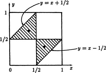
We break a stick at random in two places, what is the probability that the three pieces will form a triangle?

Naturally we assume that each break occurs uniformly in the possible range. Since it is only the relative lengths that matter we can assume that the original stick is of length 1. Let the two breaks be at points x and y, each uniformly in the unit interval (0,1). We could use symmetry and insist that x ≤ y, but rather than worry about it we will not bother to think carefully about this reduction of the problem.

FIGURE 5.2–3

The sample space of the problem is the unit square, Figure 5.2–3. If the breaks, both x and y, are at places greater than 1/2 then the other side of the triangle would be more than 1/2 and no actual triangle is possible, (no side of a triangle can be greater than the sum of the other two sides), and similarly if both breaks are at places less than 1/2. Thus the upper right and lower left are regions where the pieces could not form a triangle. The lines x = 1/2 and y = 1/2 are thus edges of regions that need to be investigated. We also require that the difference between x and y not exceed 1/2. The equations

$\begin{array}{ccc}y-x=1/2& \Rightarrow & y=x+1/2\end{array}$$\begin{array}{ccc}x-y=1/2& \Rightarrow & y=x-1/2\end{array}$

are the lines that are the edges of similar impossible regions, as shown in the Figure. To decide which of these smaller regions will let us form triangles from the three pieces, we observe that if x = 1/3, y = 2/3, or if x = 2/3, y = 1/3 then from the pieces we can make an equilateral triangle, hence these points fall in the feasible regions. The area of each is 1/8, so that the total probability of successes is (we started with unit area)

$P=1/4$

Is this answer reasonable? Let x fall in either half of the length; half the time y will fall there too, and no triangle will be possible, so already we see that the probability must be less than 1/2. If the two places of the breaks, x and y, are in opposite halves of the stick, still they must not be too far apart. Hence the 1/4 seems reasonable.

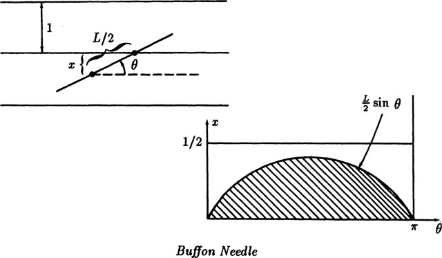
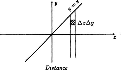
Example 5.2–4    The Buffon Needle

The famous French naturalist Buffon (1707–1788) suggested the following Monte Carlo determination of the number π. Imagine a flat plane ruled with parallel lines having unit spacing. Drop at random a needle of length L ≤ 1 on the plane. What is the probability of observing a crossing?

“At random” needs to be thought about. It seems to mean that the center of the needle is uniformly placed with respect to the set of lines, and that the angle θ that the needle makes with the direction of the lines is uniform, and by symmetry we might as well suppose that the angle is uniform in the interval (0, π). Figure 5.2–4 shows the situation. There will be a crossing if and only if the distance x from the center of the needle to the nearest line is less than L/2 sin θ. Thus the boundary in the sample space between success and failure is the curve

FIGURE 5.2–4

$x=(L/2)\sin \theta$

Since the angle runs between 0 and π the area for success is

$\begin{array}{c}A={{\displaystyle {\int }_0^{\pi }(L/2)\sin \theta d\theta =(L/2)(-\cos \theta )}|}_0^{\pi }\\ =L\end{array}$

The total area of sample space of trials is π/2, so the ratio of the success area to the total sample space area is

$2L/\pi$

We can make some trials of tossing a needle and get an estimate of the definite number π. Since it is wise to have the chance of success and failure comparable, we picked L = 8/10 and ran the following trials. We see that the first two 100 trials in Table 5.2–2 are unlikely, but gradually the results are swamped by the law of large numbers (see Section 2.8).

TABLE 5.2–1

Successes	Total	Estimate of π
43	100	3.7209
87	200	3.6782
142	300	3.3803
192	400	3.3333
246	500	3.2520

Do not think that running many cases will produce an arbitrarily good estimate of π; it is more a test of the particular random number generator in the computer! Thus these Monte Carlo runs are useful for getting reasonable estimates, and for checking a computation to see that gross mistakes have not been made, but they are not, without careful modification, an efficient way of computing numerical constants like π.

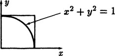
Example 5.2–5    Another Monte Carlo Estimate of π

There is a simpler way of estimating π by Monte Carlo methods than Buffon’s needle. Suppose we take two random numbers x_i, and y_i between 0 and 1 and regard them as the coordinates of a point in the plane. The probability that the random point will lie within the arc of the circle, (x > 0, y ≥ 0)

$x^2+y^2=1$

is exactly π/4 (see Figure 5.2–5).

FIGURE 5.2–5

To check the model we simulated the experiment on a small computer. The variance of the Binomial trials is {npq}^1/2, and this leads to

$\sqrt{\pi pq}=\sqrt{\frac{\pi }{4}\left(1-\frac{\pi }{4}\right)}n=0.411\dots \sqrt{n}$

The following table is the results.

TABLE 5.2–2

	Experiment		Theory
Trials	Successes	π (Estimate)	Successes	$\sqrt{npq}$
100	82	3.28	78.5	4.11
200	160	3.20	157.1	5.81
300	245	3.2667	235.6	7.11
400	323	3.23	314.2	8.21
500	407	3.256	392.7	9.18
600	482	3.2133	471.2	10.1
700	557	3.1829	549.8	10.9
800	636	3.18	628.3	11.6
900	707	3.1422	706.9	12.3
1000	788	3.152	785.4	13.0

The table indicates that the experimental data is close to the theoretical values and is generally within the likely distance from the expected value given in the last column. Thus we have again verified the model of probability we used.

Notice that in the Examples 5.2–1 and 5.2–2 we normalized each random variable while in Example 5.2–3 we merely took the ratio of area of the successes to the total area. It is necessary that you see that these two methods are equivalent. The normalization at each stage adds, perhaps, some clarity and security since you have to think oftener, but taking the ratio is often the simplest way to get the probability of a success—always assuming that the probability distribution is uniform. If it is not then the simple modification of including the weight factor in the integrals is obvious and need not be discussed at great length.

Example 5.2–6    Mean and Variance of the Unit interval

Given the continuous probability distribution

$\begin{array}{cc}p(x)=1& (0\le x\le 1)\end{array}$

what is the mean and variance?

The mean is given by (sums clearly go into integrals)

$\mu ={\displaystyle {\int }_0^{1}xp(x)dx}={\displaystyle {\int }_0^{1}xdx=1/2}$

For the variance we have, similarly,

${\sigma }^2={\displaystyle {\int }_0^1{(x-1/2)}^{2}p(x)dx}$${{\displaystyle {\int }_0^1{(x-1/2)}^{2}dx={(x-1/2)}^3/3}|}_0^1=1/12$

Exercises 5.2

5.2–1 A board is ruled into unit squares and a disc of a radius a < 1 is tossed at random. What is the probability of the disc not crossing any line? Plot the curve as a function of a. When is the chance 50–50? Ans. p = (1 – a)², $a=1-1/\sqrt{2}$.

5.2–2 Same as 5.2–1 except the board is ruled into equilateral triangles of unit side.

5.2–3 Same as 5.2–1 except regular hexagons.

5.2–4 Given a circle A of radius a with a concentric circle B of radius b < a, what is the probability that a coin of radius c(c < b) when tossed completely in A will not touch the edge of circle B? What is the 50–50 diameter? Ans. If a > b + 2c then P = {{a + c)² − 4bc}/a², if a ≤ b + 2c then P = (a – c)²/a².

5.2–5 Analyse the Buffon needle problem if you assume that one end of the needle is uniformly at random instead of the middle.

5.2–6 A circle is inscribed in a square. What is the probability of a random point falling in the circle?

5.2–7 A sphere is inscribed in a cube. What is the probability of a random point falling in the sphere?

5.2–8 In Example 5.2–6 the square is inscribed in another circle what is the probability of being in the square and not in the inner circle?

5.2–9 Sketch the sample space of Example 5.2–2.

5.2–10 Two people agree to meet between 8 and 9 p.m., and to wait a < 1 fraction of an hour. If they arrive at random what is the probability of meeting? Ans. a(2 – a).

5.2–11 A piece of string is cut at random. Show that the probability that ratio of the shorter to the longer piece is less than 1/3 is 1/2.

5.2–12 A random number is chosen in the unit interval. What is the probability that the area of a circle of this radius is less than 1? Ans. $1/\sqrt{p}$.

5.2–13 The coefficients are selected independently and uniformly in the unit interval. What is the probability that the roots of

$a{x}^2+2bx+c=0$

are real? Ans. 5/9.

5.2–14 Same as 5.2–13 except the equation ax² + bx + c = 0. Ans. (5 + 6/n2)/36 = 0.2544…

5.2–15 As in Example 5.2–1 you pick a random angle, but this time you pick a distance selected uniformly in the range 0 < x < 1. What is the expected distance from the river?

5.2–16 Two random numbers are selected from the interval 0 < x < 1. What is the probability that the sum will be less than 1?

5.2–17 Three random numbers are selected uniformly from the interval 0 < x < 1. What is the probability that the sum will be less than 1? Ans. 1/3!.

5.2–18 Select two random numbers from the interval 0 < x < 1. What is the probability that the product is less than 1/2?

5.2–19 If a point is selected in a circle with a probability density proportional to the radius, what is the normalizing factor?

5.2–20 Same as Exercise 5.2–19 except for a sphere.

5.2–21 Same as Exercise 5.2–17 except n numbers are selected. Ans. 1/n!.

5.3    Some Paradoxes

We have been fairly glib about the assignment of a uniform probability in a finite interval. As the following examples show, the troubles that can arise are more subtle than most people initially think. See also [St].

Example 5.3–1    Bertrand’s Paradox

The probabilist Bertrand asked the question, “If you draw a random chord in a circle what is the probability that it is longer than the side of the equilateral triangle that you can draw in the same circle?” The equilateral triangle scales the problem so that the probability is independent of the radius of the circle.

FIGURE 5.3–1

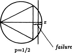
There are three different ways of reasoning. In the first, Figure 5.3–1, we select the position where the chord cuts the radius that is perpendicular to the chord, and assume that this is the equally likely choice. We see, from the geometry, that the probability is exactly 1/2.

FIGURE 5.3–2

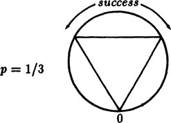
The second way is to suppose that one point on the circumference is picked arbitrarily, and assume that the other intersection is uniformly spread around the circumference. From Figure 5.3–2 we see that the probability is exactly 1/3.

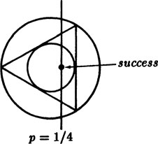
The third way we assume that the middle of the chord is spread uniformly around the inside of the circle. From Figure 5.3–3 we see that the probability is 1/4.

FIGURE 5.3–3

This is a famous paradox, and shows that when the chord is chosen at random the question of what is to be taken as uniform is not as simple as one could wish. The three different answers, 1/2, 1/3 and 1/4, can all be defended, and they are not even close to each other!

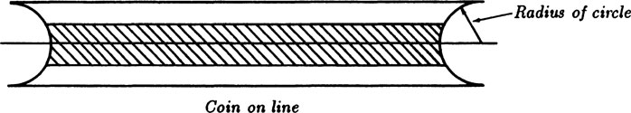
Suppose we make the apparently reasonable proposal that if A is random with respect to B, then B is random with respect to A—and we hope that the “uniform assigments” also agree. We therefore invert the Bertrand random chord tossing, and think of a line as fixed and toss a circle. If an intersection is to occur then the center of the circle should occur uniformly in the area about the line. To be concrete we imagine a line segment of finite length, and toss a coin of unit radius on the floor. We count only those trials where the coin corsses the line and forms a chord. We see that the chord will be longer than the corresponding triangle when the center is within a distance of 1/2 of the radius to the line, and have in Figure 5.3–4 allowed for the end effects of the finite line. As the line gets longer and longer, the end effects decrease relative to the rest of the experiment, so we look at the main part to see that the probability will approach 1/2. Thus we get one of Bertrand’s answers. You may think that this is the “correct answer,” but it shows that even the principle “A random with respect to B implies B random with respect to A” does not carry over to the words “uniformly random.” Indeed, if A is always 1 and B is a random number chosen uniformly in (0 < x < 1), then B is random with respect to A, but A is not random with respect to B.

FIGURE 5.3–4

The Bertrand paradox is not presented merely to amused you; it is something for you to worry about if you ever plan to model the real world by a probability model and then act on the results. Just how will you choose the assignment of the probabilities, since different assignments can give significantly different results? In computer simulations all too often the actual randomness is left to some programmer who is interested in programming and not in the relevance of the model to reality. Because of this, most simulations that use random numbers are suspect unless a person with an intimate understanding of the real situation being modeled examines the way the randomness enters into the computation. There is, so far as the author knows, no simple solution to the situation that the assignment of the random choice may not be left to the programmer to do the obvious; every assignment of a probability distribution must be carefully considered if you are to act responsibly on the results of a simulation. Symmetry was used earlier to justify the uniform distribution of a random variable; later in Chapters 6, 7 and 8 we will give further discussions of how to choose the initial random distributions.

Apparently we cannot talk with any mathematical rigor about the probability of choosing a random point, but we can accumulate the probability in intervals. In particular we define the cumulative probability between—∞ and x as _x

$\mathrm{Pr}\{-\infty \le t\le x\}=P(x)={\displaystyle {\int }_{-\infty }^{x}p(t)dt}$

for some probability density distribution p(x) where, of course,

${\displaystyle {\int }_{-\infty }^{\infty }p(t)dt=1}$

Thus the probabilty of falling in an interval (a, b) is

${\displaystyle {\int }_a^{b}p(t)dt=P(b)-P(a)}$

If we think of the derivative of the cumulative probability function (except at isolated points for practical functions) we have again the probability density function (lower case)

$p(x)$

In the infinitessimal notation of scientists and engineers we can talk about the probability of being in an interval dx as being

$p(x)dx$

but not about the probability at a point. Talking about the probability density p(x) is very convenient, but careful thinking requires us to go to the integral form whenever there is any doubt about what is going on.

We now turn to a classic problem due to Lewis Carroll (Charles Dodson, the Oxford mathematician) which illustrates the danger of using the idea of a random point in a plane.

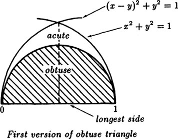
Example 5.3–2    Obtuse Random Triangles

Lewis Carroll posed the problem: if you select three random points in a plane what is the probability that the triangle will be obtuse?

For a long time the standard reasoning was to place the x-axis of a cartesian coordinate system along the longest side of the triangle, and the origin at the vertex joining the second longest side. We will scale the longest side to be of unit length since it is only the ratio of areas that will matter. Then looking at the Figure 5.3–5 we see that the third point must fall inside the circle of unit radius about the origin. But the point must also fall within a similar circle centered about the other end of the longest side. We now remember that the angle in a semicircle is a right angle, hence the circle of half the radius marks the boundary between obtuse and acute angles. The figure shows the region of obtuse angles. By symmetry it is enough to use only the upper half of the plane. The area of all the possible triangles is given by

FIGURE 5.3–5

$\text{Area}=2{\displaystyle {\int }_{1/2}^1\sqrt{(1-x^2)}dx}$

Using the standard substitution of x = sin t we get

$\text{Area}=2{\displaystyle {\int }_{\pi /6}^{\pi /2}{\cos }^{2}tdt}$

Using the half angle substitution we have

$\begin{array}{c}\text{Area}={\displaystyle {\int }_{\pi /6}^{\pi /2}(1+\cos 2t)dt}\\ =\{\pi /2-\pi /6\}+(1/2)\{\sin \pi -\sin \pi /3\}\\ =\pi /3-\frac{\sqrt{3}}{4}\end{array}$

Now the area where the obtuse triangles occur is clearly π/8, so we have the probability of an obtuse triangle is

$\frac{\frac{\pi }{8}}{\frac{\pi }{3}-\frac{\sqrt{3}}{4}}=0.639\dots$

FIGURE 5.3–6

This solution was widely accepted until someone thought to compute the answer taking the x-axis along the second longest side with unit length, and the vertex at the junction of that side with the shortest side. From Figure 5.3.6 we see that the longest side forces the other vertex to be outside a circle of radius 1 about the point x = 1, but that it must also lie inside a circle of unit radius about the origin since the shortest side is less than 1. The Figure shows the obtuse triangle area as shaded, and it is only the contiguous small area to the right of the y-axis that has acute angles. For this small area we have the integral

${\displaystyle {\int }_0^{1/2}\left[\sqrt{(1-x^2)}-\sqrt{\{(1-{(1-x)}^2\}}\right]dx}$

In the first integral we use again x = sin t, and in the second integral we use 1 – x = sin t. We get

${\displaystyle {\int }_0^{\pi /6}{\cos }^{2}tdt}-{\displaystyle {\int }_{\pi /6}^{\pi /2}{\cos }^{2}tdt}$

Again using the half angle substitution we get

$\frac{\sqrt{3}}{4}-\frac{\pi }{12}$

for this small sector. Hence the probability of an obtuse angled triangle is

$(\text{Area of success)/(total area)}=\frac{\frac{\pi }{4}}{\frac{\pi }{6}-\frac{\sqrt{3}}{2}}=0.821\dots$

This is very different from the first answer, and a simple look at the two figures will show that the two probabilities are indeed quite different.

What is wrong? It is not the choice of coordinate systems, it is the idea that you can choose a random point in the plane. Where is such a point? It is farther out than any number you can mention! Hence the distance between the points is arbitrarily large—the triangle is practically infinite and the assumptions of the various steps, including supposing that the side chosen is of unit length, are dubious to say the least.

It is significant that the first standard solution offered for the Lewis Carroll problem was accepted for so long, and it indicates the difficulty of using probability in practice, especially continuous probability. You need to be very careful whenever you come in contact with the infinite.

If we attempt to do a Monte Carlo simulation by choosing points in a square of sides 2N, for example, and letting the length of the side approach infinity we find from the random number generator we get a number x between 0 and 1, and to get to the interval—N to N we must use

$(2x-1)N$

By rearranging things a bit we see that we will always (for the uniform distribution) reduce the problem to the unit square and the factor N will drop out. For this situation we would get an answer for the probability of an obtuse triangle. But if we had chosen a circle instead of the square we would have gotten a different answer! If the difference between the answers for the square and circle is not obvious, then consider a long, flat rectangle and let the size approach infinity while keeping the “shape” of the rectangle constant. The probability of an obtuse triangle in a long, low rectangle is very high and depends on the shape of the rectangle. Hence, just which shape should we choose to let approach infinity? The answer clearly depends on this choice of shape and not on the size of the figure.

Example 5.3–3    A Random Game

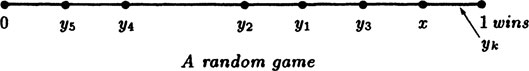
In this game I choose a random number x uniformly between 0 and 1. You then begin to pick uniformly distributed random numbers y_i from the same unit interval and are paid one unit of money for each trial until your y_i is at least as large as my x, Figure 5.3–7. If it is to be a fair game then what price should I ask? Alternately, how many trials can you expect to make until your y_i ≥ x?

FIGURE 5.3–7

For any given x that I pick, what is the probability that you will get a number y_i, larger that x and hence end the game? Since we are assuming a uniform distribution, the probability is just the length of the interval for failure. It is simply

$\text{Prob}\{y_i\ge x\}=1-x$

The expected number of trials for any fixed x (other than x = 1) is the reciprocal of the probability of the event (see 4.2–3); hence your expected gain is, for my y,

$1/(1-x)-1=x/(1-x)$

To get the expected value for the game we average this over all possible choices of my x

${{\displaystyle {\int }_0^1\frac{x}{1-x}dx=-x-\mathit{ln\hspace{0.17em}}(1-x)}|}_0^1=\infty$

Few people would play this fair (?) game with the infinite entry fee!

We can examine how this happens by dropping back to finite problems. There are several ways of doing this, and we shall examine two of them.

Suppose first that there are only a finite number of numbers in the unit interval, say N equally spaced numbers (0 ≤ x < 1). The numbers are therefore 0/N, 1/N, 2/N,…, (N − 1)/N. I must allow your sequence of numbers selected from m/M, (m = 0,1,2,.. .N − 1) to end on an equality since otherwise if my x is the largest number, (N− 1)/N, then you could never exceed it and you would be paid forever! For my given x = k/N, (k = 0,1,…, N− 1), you have the probability

$(N-k)/N$

of getting a single choice at least as large as my x. The expected number of trials will be for my particular choice x

$\text{Expected number of trials before a failure}=N/(N-k)-1$

Summed over all my x, meaning k, we get

$\text{Average expected number of trials}=\frac{1}{N}{\displaystyle \sum _{k=0}^{N-1}\left\{\frac{N}{N-k}-1\right\}}$

If we set k’ = N—k in the first sum, then

$\text{Average expected number of trials}={\displaystyle \sum _{k^{\prime }=1}^N\frac{1}{k^{\prime }}-1}$

We can, by the result in Appendix 1.A, approximate the sum by the midpoint integration formula to get

$(1/N){\displaystyle {\int }_{1/2}^{N+1/2}\frac{1}{x}dx-1~\mathit{ln\hspace{0.17em}}(2N+1)-1}$

As the number of points, N, used in the unit interval increases, the expected number of trials goes to infinity like ln N. This is much like the St. Petersburg paradox (Section 4.8). We also note that as N approaches infinity we are measuring the interval with a spacing 1/N and we do not involve the discrete vs. the continuous.

A second approach is to choose my number from some fraction of the unit line, say (0 ≤ x ≤ a < 1), which amounts to taking my number from (0 ≤ x ≤ 1) and multiplying by a < 1. Now your y_i must exceed my number ax. We are led to the integral

$\frac{1}{a}{\displaystyle {\int }_0^a\frac{1}{1-x}dx=\frac{1}{a}\mathit{ln\hspace{0.17em}}\left\{\frac{1}{1-a}\right\}}$

and as a → 1 this again heads for infinity.

Again we see that even in simple problems you get results that you would not act on in the real world. These particular paradoxical results are easy to spot because they involved an infinity that is in the open; how can you hope to spot similar errors when the results are not so clearly displayed?

Probability applications are dangerous, but in practice there are many situations where there is no other basis for action and where also no action is very dangerous. It is for such reasons that we continually examine the foundations of our assumptions and the way we compute. Dropping back to one or more finite models (as does the calculus) often seems to shed a great deal of light on the situation, and is highly recommended in practice where the consequences of the calculation are important. It is the actual application that indicates the finite model to use and determines your untimate actions.

5.4    The Normal Distribution

The integral

$I={\displaystyle {\int }_{-\infty }^{\infty }{e}^{-x^2/2}dx}$

(5.4–1)

will occur frequently and we need to know its value even though we cannot do the indefinite integration in closed form. There is a standard trick for the evaluation. We compute the square of the integral and then convert to the double integral form

$\begin{array}{c}{I}^2={\displaystyle {\int }_{-\infty }^{\infty }{e}^{-x^2/2}dx}{\displaystyle {\int }_{-\infty }^{\infty }{e}^{-y^2/2}dy}\\ ={\displaystyle {\int }_{-\infty }^{\infty }{\displaystyle {\int }_{-\infty }^{\infty }{e}^{-(x^2+y^2)/2}dydx}}\end{array}$

We next formally convert to polar coordinates (since the sum of the squares strongly suggests this)

$\begin{array}{c}{I}^2={\displaystyle {\int }_0^{2\pi }{\displaystyle {\int }_0^{\infty }{e}^{-r^2/2}rdrd\theta }}\\ =2\pi {\displaystyle {\int }_0^{\infty }{e}^{-r^2/2}rdr}\\ ={2\pi \left(-e^{-r^2/2}\right)|}_0^{\infty }=2\pi \end{array}$

Hence we have for (5.4–1)

$I={\displaystyle {\int }_{-\infty }^{\infty }{e}^{-x^2/2}dx=\sqrt{2\pi }}$

(5.4–2)

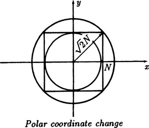
Since this is an important result we need to examine carefully the change of the integration from repeated to double, and the change to polar coordinates. We therefore begin with the finite integral corresponding to (5.4–1)

$I(N)={\displaystyle {\int }_{-N}^N{e}^{-x^2/2}dx}$

and repeat the steps. When we get to the change to polar coordinates we look at Figure 5.4–1. We get the bounds that the integral over the inner circle is less than the integral over the square, which in turn is less than the integral over the outer circle. Doing the angle integration we have

$2\pi {\displaystyle {\int }_0^N{e}^{-r^2/2}rdr<I^2(N)<2\pi }{\displaystyle {\int }_0^{\sqrt{2N}}{e}^{-r^2/2}rdr}$

FIGURE 5.4–1

The two end integrals can be done in closed form

$2\pi \{1-e^{-N^2/2}\}<I^2(N)<2\pi \{1-e^{-N^2}\}$

In the limit as N → ∞ each end of the inequality approachs 2π, SO the middle term must too, and we are justified, this time, in the formal approach.

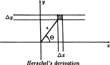
Example 5.4–1    Herschel’s Derivation of the Normal Distribution

The astronomer Sir John F. W. Herschel (1792–1871) gave the following derivation of the the normal distribution. Consider dropping a dart at a target (the origin of the rectangular coordinate system) on a horizontal plane. We suppose: (1) the errors do not depend on the coordinate system orientation, (2) errors in perpendicular directions are independent, and (3) large errors are less probable than are small errors. These seem to be reasonable assumptions.

FIGURE 5.4–2

Let the probability of the dart falling in the strip from x to x + Δx be p(x)Δx, and of falling in the strip from y to y + Δy be p(y)Δy, see Figure 5.4–2. The probability of falling in the shaded rectangle is, since we assumed the independence of the coordinate errors,

$p(x)p(y)\Delta x\Delta y=g(r)\Delta x\Delta y$

where r is the distance of the origin to the place where the dart falls. From this we conclude that

$p(x)p(y)=g(r)$

Now g(r) does not depend on the angle θ in polar coordinates, hence we have (using partial derivatives)

$\frac{\partial g(r)}{\partial \theta }=0=p(x)\frac{\partial p(y)}{\partial \theta }+p(y)\frac{\partial p(x)}{\partial \theta }$

From the polar coordinate relationships

$x=r\cos \theta$$y=r\sin \theta$

we have

$\frac{\partial p(x)}{\partial \theta }=\frac{\partial p(x)}{\partial x}\frac{\partial x}{\partial \theta }=p^{\prime }(x)(-y)$$\frac{\partial p(y)}{\partial \theta }=\frac{\partial p(y)}{\partial y}\frac{\partial y}{\partial \theta }=p^{\prime }(y)(x)$

This gives

$p(x)p^{\prime }(y)(x)-p(y)p^{\prime }(x)(y)=0$

Separating variables we have the two differential equations

$\frac{p^{\prime }(x)}{xp(x)}=\frac{p^{\prime }(y)}{yp(y)}=K$

since both sides of the equation must be equal to some constant K (the variables x and y are independent). We have, therefore, for the variable x,

$\frac{p^{\prime }(x)}{p(x)}=Kx$$\mathit{ln\hspace{0.17em}}p(x)=K{x}^2/2+C$$p(x)=A{e}^{K{x}^2/2}$

But we assumed that small errors were more probable than large ones, hence K < 0, say

$K=-1/{\sigma }^2$

and we have the normal distribution

$p(x)=A{e}^{-x^2/2{\sigma }^2}$

From the fact that the total probability must be 1 we get for the factor A

$A=1/(\sigma \sqrt{2\pi })$

Similar arguments apply to the y variable.

The derivation seems to be quite plausible, and the assumptions reasonable. We will later find (Chapter 9) other derivations of the normal distribution.

Example 5.4–2    Distance to a Random Point

Let us select independently both the x and y coordinates of a point in the x-y plane from the same normal distribution which is centered at the origin (which is no real constraint)

$p(t)=\frac{1}{\sigma \sqrt{2\pi }}{e}^{-t^2/2{\sigma }^2}$

The expected distance from the origin is then given by

$D=\frac{1}{{\sigma }^{2}2\pi }{\displaystyle {\int }_{-\infty }^{\infty }{\displaystyle {\int }_{-\infty }^{\infty }\sqrt{(x^2+y^2)}{e}^{-(x^2+y^2)/2{\sigma }^2}dydx}}$

This immediately suggests polar coordinates (where we can now do the θ integration)

$\begin{array}{c}D=\frac{1}{{\sigma }^{2}2\pi }{\displaystyle {\int }_0^{2\pi }{\displaystyle {\int }_0^{\infty }{r}^2{e}^{-r^2/2{\sigma }^2}drd\theta }}\\ =\frac{1}{{\sigma }^2}{\displaystyle {\int }_0^{\infty }{r}^2{e}^{-r^2/2{\sigma }^2}dr}\end{array}$

Set r = σt to get

$D=\sigma {\displaystyle {\int }_0^{\infty }{t}^2{e}^{-t^2/2}dt}$

Integration by parts yields easily, and use (5.4–2)

$\begin{array}{c}D=\sigma \{-t{e}^{-t^2/2}|{}_0^{\infty }+{\displaystyle {\int }_0^{\infty }{e}^{-t^2/2}dt}\}\\ =\sigma \sqrt{2\pi }\end{array}$

as the expected distance of the random point in the x-y plane from the origin.

This transformation from rectangular to polar coordinates needs some justification. We therefore, as before, adopt the calculus approach and start with the region —N to N. From Figure 5.4–2 we see that we can easily get the bounds

${\displaystyle {\int }_0^{2\pi }{\displaystyle {\int }_0^N{r}^2{e}^{-r^2/2{\sigma }^2}drd\theta }}$$<{\displaystyle {\int }_{-N}^N{\displaystyle {\int }_{-N}^N\sqrt{(x^2+y^2)}{e}^{-(x^2+y^2)/2{\sigma }^2}dydx}}$$<{\displaystyle {\int }_0^{2\pi }{\displaystyle {\int }_0^{\sqrt{2N}}{r}^2{e}^{-r^2/2{\sigma }^2}drd\theta }}$

Now as N → ∞ both end integrals approach the same limit, hence the transformation from rectangular to polar coordinates is legitimate this time.

Notice that the normal distribution has the important property that the product formula p(x)p(y) has circular symmetry.

Example 5.4–3    Two Random Samples from a Normal Distribution

Suppose we choose two random points on a line, not from a uniform infinite distribution but rather from the probability density distribution

$p(x)=\frac{1}{\sqrt{2\pi }}{e}^{-x^2/2}$

What is the expected distance between the two points?

The probability density of two independently chosen coordinates x and y from this normal distribution is their product, which is

$\frac{1}{2\pi }{e}^{-(x^2+y^2)/2}$

FIGURE 5.4–3

In the sample space of the events we have a probability distribution of points over the entire x-y plane to consider (although the two points lie on a line). See Figure 5.4–3. To get the expected distance between the two points we will have to consider points in the entire sample space plane, but to evaluate the integral we can take only y > x and use a factor of 2 in front of the integral to compensate

$2{\displaystyle {\int }_{-\infty }^{\infty }{\displaystyle {\int }_{-\infty }^y\frac{1}{2\pi }(y-x)e^{-(x^2+y^2)/2}dxdy}}$$=\frac{1}{\pi }{\displaystyle {\int }_{-\infty }^{\infty }{e}^{-x^2/2}}{\displaystyle {\int }_x^{\infty }y{e}^{-y^2/2}dydx}$$-\frac{1}{\pi }{\displaystyle {\int }_{-\infty }^{\infty }{e}^{-y^2/2}}{\displaystyle {\int }_{-\infty }^{y}x{e}^{-x^2/2}dxdy}$

where we have interchanged the limits in the first integral. Again this interchange needs to be examined, but as in the previous cases the rapid decay of the exponential term justifies the interchange. Doing the inner integrals we get (since the exponentials combine)

$\frac{1}{\pi }{\displaystyle {\int }_{-\infty }^{\infty }{e}^{-y^2}dy}+(\text{same in }x)$$=\frac{2}{\pi }{\displaystyle {\int }_{-\infty }^{\infty }{e}^{-y^2}dy}$

But this is a known integral (5.4–2) which gives, finally,

$2/\sqrt{\pi }=1.128\dots$

as the expected distance between two points chosen from a normal distribution with unit variance.

We see from these last several examples that while the idea of a random point in the infinite plane chosen from a uniform distribution can lead to peculiar results, when we choose from a reasonably restricted distribution we get reasonable results. Example 5.3–3 is another case resembling the St. Petersburg and Castle Point paradoxes. The integral for the expected value may be infinite when you are careless – even for a finite interval!

Exercises 5.4

5.4–1 Evaluate ${\displaystyle {\int }_{-\infty }^{\infty }{x}^n{e}^{-x^2/2}dx}$.

5.4–2 In Bertrand’s paradox compute the expected values of the chord in the three cases. Ans. π/2 = 1.5708…, 4/π = 1.2732…, 4/3

5.4–3 Why do you have trouble with the random triangle when you choose the shortest side?

5.4–4 Rework the random game if you must get a number less than mine.

5.4–5 In a circle of radius 1 the probability density function along a radius is proportional to 1/r. What is the constant of proportionality?

5.4–6 As in Exercise 5.4–5 except proportional to r.

5.4–7 As in Exercise 5.4–5 except for a sphere.

5.4–8 As in Exercise 5.4–6 except for a sphere.

5.4–9 If p(x) = e^-x, (0 ≤ x ≤ ∞), find the expected distance from the random point to the origin.

5.4–10 Same as Exercise 5.4–6 except the distance from 1.

5.4–11 Same as Exercise 5.4–7 except the point a. Ans. a− 1 + 2 exp(—a).

5.4–12 What is the expected distance between two points chosen at random on a sphere? Note that you can assume that there is a great circle going through the two points, but that you need to consider elementary areas and not simply points.

5.4–13 Find the inflection points of the normal probability density function.

5.4–14 Plot the normal density function using equal sized units on both axes.

5.5    Distribution of Numbers

When we deal with numbers in science and engineering we generally use the scientific notation and then, contrary to the usual belief, the distribution of a set of naturally occuring numbers is seldom uniform, rather most of the time the probability density of seeing a number x, where we are neglecting the exponents and looking only at the so called mantissa, is

$p(x)=\frac{1}{x\mathit{ln\hspace{0.17em}}10}$

(5.5–1)

when we regard the numbers as lying between 1 and 10). This is naturally called the reciprocal distribution.

Again, we are working in the floating point (or scientific) notation that is used in almost all practical computation, and we are concerned with the decimal digits and not with the exponent. With the increasing use of computers this is an important topic having many consequences in numerical computations, including roundoff propagation studies.

Integrating the distribution (5.5–1) to get its cumulative distribution we get

$\begin{array}{cc}P(x)=\frac{\mathit{ln\hspace{0.17em}}x}{\mathit{ln\hspace{0.17em}}10}={\log }_{10}x,& P(10)=1\end{array}$

(5.5–2)

From this it follows that the probability of seeing a leading digit N is

Pr (leading digit is N) = log(N + 1) – log N = log(1 + 1/N)

To check this experimentally we took the 50 physical constants from the NBS Handbook of Mathematical Functions (1964). We got the following table 5.5–1

TABLE 5.5–1

Leading digit	Observed	Theoretical	Difference
1	16	15	1
2	11	9	2
3	2	6	–4
4	5	5	0
5	6	4	2
6	4	3	1
7	2	3	–1
8	1	3	–2
9	3	2	1
	50	50	0

We see from this simple table that the reciprocal distribution is a reasonably accurate approximation to the physical constants tabulated in the book.

But this distribution is also a property of our number system as can be seen from the following series of results. We will want, ultimately, the distribution of a product of two numbers x and y drawn from the two distributions f(x) and g(y) so we examine this first.

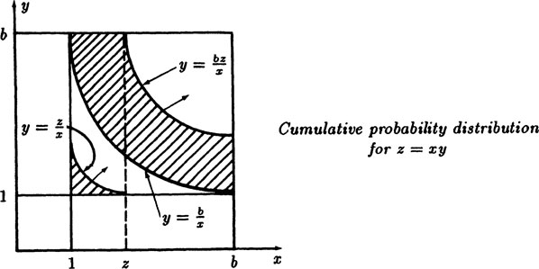
Example 5.5–1    The General Product

Consider the product z = xy when x is from the distribution f(x) and y from g(y) and where the product has been reduced to the standard floating point format. We examine the cumulative distribution P(z) of the mantissa, remembering that the same number z can arise from various places in the x-y plane (1 ≤ x,y ≤ 10,) and we need to watch especially those that come from a shift when the product is reduced to the standard floating point format. For generality we work in base b (typically b = 2,4, 8, 10, or 16), and assume that the numbers lie bewteen 1 and b (though on computers the standard notation is often from 1/b to 1).

When does a shift occur? Whenever the product z ≥ b. Hence the dividing line in the sample space is clearly

$z=xy=b$

FIGURE 5.5–1

This is an equilateral hyperbola shown in the Figure 5.5–1. When z < b we have the product z = xy, and when z > b we have the product z = xy/b. There are three regions that fall below z in computing the cumulative probability function P(z). These are shown in the figure. The corresponding integrals are

$P(Z<z)={\displaystyle {\int }_1^z{\displaystyle {\int }_1^{z/x}f(x)g(y)dydx}}$$+{\displaystyle {\int }_1^z{\displaystyle {\int }_{b-x}^{b}f(x)g(y)dydx}}$$+{\displaystyle {\int }_z^b{\displaystyle {\int }_{b/x}^{bz/x}f(x)g(y)dydx}}$

If G(y) is the cumulative distribution of g(y), that is

$\begin{array}{ccc}G(y)={\displaystyle {\int }_1^{y}g(t)dt,}& G(1)=0,& G(b)=1\end{array}$

then we have, on doing the integrations with respect to y,

$P(Z<z)={\displaystyle {\int }_1^{z}f(x)\{G(z/x)-G(1)+G(b)-G(b/x)\}dx}$$+{\displaystyle {\int }_z^{b}f(x)\{G(bz/x)-G(b/x)\}dx}$$={\displaystyle {\int }_1^{z}f(x)\{G(z/x)+1-G(b/x)\}dx}$$+{\displaystyle {\int }_z^{b}f(x)\{G(bz/x)-G(b/x)\}dx}$

To get the probability density h(z) we differentiate with respect to z, remembering all the details of differentiating an integral with respect to a parameter. We get

$h(z)=f(z)\{G(1)+1-G(b/z)\}-f(z)\{G(b)-G(b/z)\}$$+{\displaystyle {\int }_1^{z}f(x)\{g(z/x)(1/x)\}dx}$$+{\displaystyle {\int }_z^{b}f(x)\{g(bz/x)(b/x)\}dx}$$={\displaystyle {\int }_1^{z}f(x)\{g(z/x)(1/x)\}dx}$$+{\displaystyle {\int }_z^{b}f(x)\{g(bz/x)(b/x)\}dx}$

(5.5–3)

This is the formula for the density distribution h(z) for the product xy in floating point (scientific) notation. It does not look symmetric in the two variables x and y as it should since xy = yx, but changing variables in the integrands will convince you that the formula has the required symmetry.

Example 5.5–2    Persistence of the Reciprocal Distribution

If we assume that one of the variables, say y, is from the reciprocal distribution, that is

$g(y)=1/(y\mathit{ln\hspace{0.17em}}b)$

then we have for the distribution of the product (see 5.5–3)

$h(z)={\displaystyle {\int }_1^{z}f(x)\{x/(z\mathit{ln\hspace{0.17em}}b)\}\{1/x\}dx}$$+{\displaystyle {\int }_z^{b}f(x)\{x/(bz\mathit{ln\hspace{0.17em}}b)\}\{b/x\}dx}$$=1/(z\mathit{ln\hspace{0.17em}}b)\left\{{\displaystyle {\int }_1^{z}f(x)dx}+{\displaystyle {\int }_z^{b}f(x)dx}\right\}$$=1/(z\mathit{ln\hspace{0.17em}}b)$

(5.5–4)

Thus if one factor of the product is from the reciprocal distribution then the product has the reciprocal distribution.

Example 5.5–3    Probability of Shifting

In forming a product of two numbers on a computer a shift to reduce the product to the standard format requires extra effort and possibly extra time. What is the probability of a shift? By placing the point of the number system behind or before the leading digit we can change from the probability of a shift to its complement probability.

If both numbers are from general distributions then the probability of no shift is the area under the curve y = b/x (see Figure 5.5–1)

$\mathrm{Pr}(\text{shift})={\displaystyle {\int }_1^b{\displaystyle {\int }_1^{b/x}f(x)g(y)dydx}}$

If both factors are from the reciprocal distribution then we have

$\begin{array}{ll}\mathrm{Pr}\text{(shift)}\hfill & ={\displaystyle {\int }_1^b{\displaystyle {\int }_1^{b/x}1/(x\mathit{ln\hspace{0.17em}}b)1/(y\mathit{ln\hspace{0.17em}}b)dydx}}\hfill \\ \hfill & =\frac{1}{{(\mathit{ln\hspace{0.17em}}b)}^2}{{\displaystyle {\int }_1^b(1/x)\mathit{ln\hspace{0.17em}}y}|}_1^{b/x}dx\hfill \\ \hfill & =\frac{1}{{(\mathit{ln\hspace{0.17em}}b)}^2}{\displaystyle {\int }_1^b(1/x)\{\mathit{ln\hspace{0.17em}}b-\mathit{ln\hspace{0.17em}}x\}dx}\hfill \\ \hfill & =\frac{1}{{(\mathit{ln\hspace{0.17em}}b)}^2}\left[{\mathit{ln\hspace{0.17em}}b\mathit{ln\hspace{0.17em}}x-{(\mathit{ln\hspace{0.17em}}x)}^2/2|}_1^b\right]\hfill \\ \hfill & =\frac{1}{{(\mathit{ln\hspace{0.17em}}b)}^2}[{(\mathit{ln\hspace{0.17em}}b)}^2-{(\mathit{ln\hspace{0.17em}}b)}^2/2]\hfill \\ \hfill & =1/2\hfill \end{array}$

Thus if both numbers come from the reciprocal distribution then it is a matter of indifference whether or not the point is before or behind the leading digit. For other distributions this is not true.

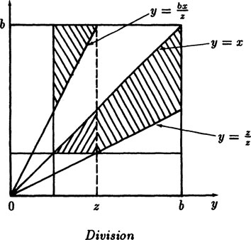
Example 5.5–4    The General Quotient

For the quotient

$z=x/y$

FIGURE 5.5–2

we first draw the picture, Figure 5.5–2 showing the various regions and the equations bounding the regions. As before we begin with the cummulative probability distribution which is

$H(z)={\displaystyle {\int }_1^z{\displaystyle {\int }_{bx/z}^{b}f(x)g(y)dydx}}$$+{\displaystyle {\int }_1^z{\displaystyle {\int }_1^{z}f(x)g(y)dydx}}$$+{\displaystyle {\int }_z^b{\displaystyle {\int }_{x/z}^{x}f(x)g(y)dydx}}$

Again, following the earlier model we let G(y) be the cummulative distribution of g(y), and doing the dy integrations we get

$H(z)={\displaystyle {\int }_1^{z}f(x)\{G(b)-G(bx/z)+G(x)-G(1)\}dx}$$+{\displaystyle {\int }_z^{b}f(x)\{G(x)-G(x/z)\}dx}$

Differentiating to get the probability density h(z) we get

$h(z)=f(z)\{G(b)-G(b)+G(z)-G(1)-G(z)+G(1)\}$$+{\displaystyle {\int }_1^{z}f(x)g(bx/z)(bx/z^2)dx}$$+{\displaystyle {\int }_z^{b}f(x)g(x/z)(x/z^2)dx}$$=\frac{b}{z^2}{\displaystyle {\int }_1^{z}xf(x)g(bx/z)dx}$$+\frac{1}{z^2}{\displaystyle {\int }_z^{b}xf(x)g(x/z)dx}$

(5.5–5)

This is the general formula for the probability of a mantissa of the size z from a quotient z = x/y.

As a check on the formula suppose g(y) is the reciprocal distribution

$g(y)=1/(y\mathit{ln\hspace{0.17em}}b)$

We put this into (5.4–5) to get, after a lot of cancellation,

$\begin{array}{c}h(z)=\frac{1}{z\mathit{ln\hspace{0.17em}}b}\left\{{\displaystyle {\int }_1^{z}f(x)dx}+{\displaystyle {\int }_z^{b}f(x)dx}\right\}\\ =\frac{1}{z\mathit{ln\hspace{0.17em}}b}\end{array}$

Hence we get the reciprocal distribution so long as the denominator is from the reciprocal distribution. This increases our faith in (5.5–5).

Exercises 5.5

5.5–1 Find the formula for the probability of a shift if only one factor of a product is from the reciprocal distribution. Apply to one from the flat distribution.

5.5–2 If the numerator is 1 and the denominator comes from the reciprocal distribution find the distribution.

5.5–3 Discuss the question of a shift for quotients.

5.5–4 Compute the probability of a shift for a product if both numbers are from a flat distribution.

5.5–5 Tabulate the probability of a shift if both factors are from flat distribution for b = 2, 4, 8, 10, and 16.

5.6    Convergence to the Reciprocal Distribution

How fast do we approach the reciprocal distribution from any other distribution? Is the reciprocal distribution stable in practice? These are natural questions to ask. We will first examine how, starting from the flat distribution, we approach the reciprocal distribution as we take more and more products.

Example 5.6–1    Product of Two Numbers from a Flat Distribution

Suppose we start with two factors from a flat distribution, that is f(x) = 1/(b − 1) = g(y). Then the product formula gives

$\begin{array}{c}h(z)=\frac{1}{{(b-1)}^2}\left\{{\displaystyle {\int }_1^{z}1/xdx}+{\displaystyle {\int }_z^{b}b/xdx}\right\}\\ =\frac{1}{{(b-1)}^2}\{\mathit{ln\hspace{0.17em}}z+b(\mathit{ln\hspace{0.17em}}b-\mathit{ln\hspace{0.17em}}z)\}\\ =\frac{1}{{(b-1)}^2}\{b\mathit{ln\hspace{0.17em}}b-(b-1)\mathit{ln\hspace{0.17em}}z\}\end{array}$

For base 10, for example this is

$h(z)=\frac{10\mathit{ln\hspace{0.17em}}10-9\mathit{ln\hspace{0.17em}}z}{81}$

(5.6–1)

We can check this kind of a result by forming all possible products from the uniform distribution using 1, 2, 3, or even 4 digit arithmetic. There will be a decreasing effect of the granularity of the simulation of a uniform distribution, see Example 5.6–4.

Example 5.6–2    Approach to Reciprocal Distribution in General

To discuss the rapidity of the approach to the reciprocal distribution we need a measure of the distance between two probability distributions. After some thought we introduce the distance function for the distance of a probability distribution h(z) from the reciprocal distribution of r(z)

$\text{DIST}=D\{h(z)\}=\underset{1<z<b}{\max }\left\{\left|\frac{h(z)-r(z)}{r(z)}\right|\right\}$

(5.6–2)

This measures the maximum difference between the given distribution h(z) relative to the reciprocal distribution r(z). We showed in Example 5.5–2 that

$r(z)={\displaystyle {\int }_{1}zf(x)r(z/x)(1/x)dx}$$+{\displaystyle {\int }_z^{b}f(x)r(bz/x)(b/x)dx}$

Subtract this from the formula (5.5–3) for h(z) and divide by r(z), which is not the variable of integration so it may be put inside the integrals

$\frac{\{h(z)-r(z)\}}{r(z)}$$={\displaystyle {\int }_1^{z}f(x)\{g(z/x)-r(z/x)\}/xr(z)dx}$$+{\displaystyle {\int }_z^{1}f(x)\{g(bz/x)-r(bz/x)\}\{b/xr(z)\}dx}$

(5.6–3)

But we have both

$\begin{array}{ccc}xr(z)=x/z\mathit{ln\hspace{0.17em}}b=r(z/x)& \text{and}& xr(z)/b=x/bz\mathit{ln\hspace{0.17em}}b=r(bz/x)\end{array}$

so that we have, on writing the corresponding distance function at any point x

$k(z)=\frac{\{g(z)-r(z)\}}{r(z)}$$\frac{\{h(z)-r(z)\}}{r(z)}={\displaystyle {\int }_1^{z}f(x)k\{g(z/x)\}dx}$$+{\displaystyle {\int }_z^{b}f(x)k\{g(bz/x)\}dx}$

(5.6–4)

If we assume that the distance of g(x) from the reciprocal is some number D{g(z)}, then

$\begin{array}{ll}\left|D\right\{h(z)\left\}\right|\hfill & \le D\{g(z)\}\left\{{\displaystyle {\int }_1^{z}f(x)dx}+{\displaystyle {\int }_z^{b}f(x)dx}\right\}\hfill \\ \hfill & \le D\{g(z)\}\hfill \end{array}$

(5.6–5)

and therefore the distance after a multiplication is not greater than the distance from the smaller of the distances of the product terms from the reciprocal (since f(x) and g(y) play symmetric roles).

Since g(z) and r(z) are both probability distributions the difference

$g(z)-r(z)$

in the numerators of (5.6–3) must change sign at least once in the interval (1,b) and there will usually be a lot of cancellation in the integrals where we have merely put bounds. Thus, without going into great detail, we see that a sequence of products, all drawn from a flat distribution will rapidly approach the reciprocal distribution.

Example 5.6–3    Approach from a Flat Distribution

If we start with a flat distribution for both factors, that is

$f(x)=g(x)=\frac{1}{b-1}$

then we have for the distribution of the product from Example 5.6–1,

$h(z)=\frac{[b\mathit{ln\hspace{0.17em}}b-(b-1)\mathit{ln\hspace{0.17em}}z]}{{(b-1)}^2}$

If we continue we get the distance function for k factors from a flat distribution we get

Number of factors	Distance	% of original distance
1	1.558	100.0
2	0.3454	22.2
3	0.0980	6.29
4	0.0289	1.85

This shows that when the numbers are drawn from a flat distribution the product rapidly approaches the reciprocal distribution.

For division the results are much the same, see Exercises.

Example 5.6–4    A Computation of Products from the Flat Distribution

To check the formulas and the theory we made three experiments. We divided the range into 9, 99, and 999 intervals, picked the midpoint numbers as representatives of the intervals, and formed all the possible products. We compared the results with the result of Example 5.6–1.

Table for 9 intervals

Digit	Number of cases	% of cases	Theoretical
1	19	23.457	24.135
2	16	19.753	18.321
3	11	13.580	14.545
4	9	11.111	11.738
5	7	8.642	9.501
6	7	8.642	7.640
7	3	3.704	6.047
8	6	7.407	4.655
9	3	3.704	3.418
total=	81

Table for 99 intervals

Digit	Number of cases	% of cases	Theoretical
1	2364	24.120	24.135
2	1799	18.355	18.321
3	1426	14.546	14.545
4	1143	11.662	11.738
5	931	9.499	9.501
6	756	7.714	7.640
7	584	5.959	6.047
8	462	4.714	4.647
9	336	3.343	3.418
total=	9999

Table for 999 intervals

Digit	Number of cases	% of cases	Theoretical
1	240,890	24.1373	24.135
2	182,844	18.3210	18.321
3	145,181	14.5472	14.545
4	117,124	11.7359	11.738
5	94,816	9.5006	9.501
6	76,256	7.6409	7.640
7	60,321	6.4418	6.047
8	46,478	4.6471	4.655
9	34,091	3.4159	3.418
total=	999,999

Thus we see that the granularity of the actual number system used in computers is successfully approximated by the continuous model of infinite precision – that the continuous model is robust with respect to the actual discrete computer model used in practice.

Exercises 5.6

5.6–1 Find the formula for the product of two numbers from a flat distribution, and then for four numbers.

5.6–2 The same for quotients.

5.6–3 Find the formula for the product of two numbers divided by a third.

5.6–4 Plot the difference computed in Exercise 5.6–3.

5.6–5 Plot the relative distance in Exercise 5.6–4.

5.6–6 Examine the rapidity of the approach in Exercise 5.6–3 from the flat to the limiting reciprocal distribution by trying the product of two such numbers.

5.6–7 Test Exercise 5.6–3 using 1 and 2 digit numbers.

5.6–8 Do a Monte Carlo test of Exercise 5.6–3.

5.7    Random Times

Apparently our instincts about time endow the flow of time with a bit more continuity than that of space, and we seem less likely to try to think of things happening in infinite time than on an infinite line or infinite plane. Furthermore, the Bernoulli type argument against the use of the expected value for money (Section 3.7) does not necessarily apply when we consider time. In estimating the average rate of failure of a machine the expected value is very useful and apparently is appropriate.

We first consider the following example where we pick a random time to observe.

Example 5.7–1    Sinusoidal Motion

Suppose a target is moving up and down in a sinusoid across our line of vision, and we want to hit it, but must aim and fire at a random time. We feel that it is reasonable to pick the random time in suitable half period π, which we can take from—π/2 to π/2 (this covers exactly once all values that can occur). We pick the motion as

$\begin{array}{cc}y(t)=\sin t& \left|t\right|\le \pi /2\end{array}$

which clearly exhibits the assumption of the uniformity in time. We have by elementary calculus

$t=\arcsin y$$dt/dy=\frac{1}{\sqrt{1-y^2}}$

Now the probability of finding the target at a position between y and y + Δy must be approximately

$\Delta P=\frac{1}{\pi }\frac{1}{\sqrt{1-y^2}}\Delta y$

from which the probability density is

$p(t)=\frac{1}{\pi \left|\cos t\right|}$

We see that aiming at the midpoint of the interval (the expected value) is poor policy—we should pick one or the other end. Of course, since things in practice are finite in size, we are not dealing with exact points, so we need to pick our direction in a small angle from one of the extremes, but this detail does not alter the fact that the average (expected) position is not where to aim, but rather we should aim near one of the extremes.

Although we started out with a random point in time we were apparently not seriously bothered, in this case of a periodic motion where we picked a characteristic finite interval of behavior, but it needs careful thinking to convince yourself that we are not in the same position as picking a random point on an infinite line—both the periodicity, and, to a curious extent for many people, the use of time, seems to justify the process.

We believe that in this world many events occur approximately at random times, for example the decay of a radioactive atom, the time the next telephone call is placed on a central office, the time the next “job” is submitted to a computer, the time of the next death in a hospital, the time of the next failure of a machine (or one of its parts), etc. Each seems to be more or less random. We need to develop the mathematical tools for thinking about such things, including the probability density function p(t).

We will use the standard approach of examining the finite case and then let the number of intervals approach infinity as the maximum length of an interval approaches zero—the standard method for setting up integrals.

Example 5.7–2    Random Events in Time

Consider, first, a fixed time interval (0 ≤ x ≤ t). Let it be divided into n equal-sized subintervals each of length t/n. If each subinterval has the same probability of an event occuring, say p, and they are independent (Bernoulli), then the probability of exactly k events in the n intervals is

$P_k(t)=b(k;n,p)=C(n,k)p^k{(1-p)}^{n-k}$

Now fix n and p. We next further subdivide each of the n intervals into m equal parts, and hence from the uniformity assumption we have the probability of an event in the new subintervals of length t/mn is p/m.

We have for the finer subintervals the same formula with new parameters

$P_k(t)=C(nm,t){(p/m)}^k{(1-p/m)}^{mn-k}$

It is now merely a matter of rearranging this expression before we take the limit as m → ∞. We simply write out the terms in detail and reorganize the expression

$\begin{array}{c}{P}_k(t)=\{mn(mn-1)(mn-2)\cdots (mn-k+1)/k!\}\times {\left(p/m\right)}^k{\left(1-p/m\right)}^{mn}{\left(1-p/m\right)}^{-k}\\ =n(n-1/m)(n-2/m)\cdots \times (n-(k-1)/m)\{p^k/k!\}{[{\left(1-p/m\right)}^{-m/p}]}^{-np}{\left[1-p/m\right]}^{-k}\end{array}$

Now we let m → ∞, remembering that k is fixed, and we get

$P_k(t)\to n^k[p^k/k!]e^{-np}[1]$$=\frac{{(np)}^k}{k!}{e}^{-np}$

But recall that np is the expected number of successes in the original interval t. Hence if we now write a as the expected number of events in unit time we have

$np=at$

and hence

$P_k(t)=\frac{{(at)}^k}{k!}{e}^{-at}$

(5.7–1)*

as the limiting probability of k events in an interval of length t.

If we set the number of events in time t, at = k, we will get

$P\{X=k\}=\frac{{\lambda }^k{e}^{-\lambda }}{k!}$

The generating funtion of this Poisson distribution is (t in no longer time)

$\text{G}\text{.F}\text{.}={\displaystyle \sum _0^{\infty }{t}^k{\lambda }^k{e}^{-\lambda }/k!=e^{(\lambda -1)t}}$

To understand this formula, (and the fact that unusual events have to happen frequently according to this formula) we examine the probability of 0, 1, 2,… occurrences in the time t = 1/a (which is the time interval in which you expect a single event to occur). We have

$P_0(1/a)=1/e=0.3679$$P_1(1/a)=1/e=0.3679$$P_2(1/a)=1/2e=0.1839$$P_3(1/a)=1/3!e=0.0613$$P_4(1/a)=1/4!e=0.0153$$P_5(1/a)=1/5!e=0.0031$$\begin{array}{cc}\cdots & \cdots \end{array}$

(5.7–2)

Thus, in an interval in which you expect to see a single event the actual probabilities of no event and of 1 event are the same, each about 37%. The probability of 2 events is only half that of no event, about 18%; and of 3 events 1/6 that of no event, about 6%; etc. In words, in an inteval in which the expected number of events is 1 you can expect 3 events about 6% of the time (in the time interval t = 1/a). The bunching of events is much more likely than most people expect.

We also see that the sum of all the values is exactly 1, since the system must produce one of the events (outcomes) Pk(t) for each t. To demonstrate this mathematically we recall that the terms of the exponential series for e are simply 1/n!

The model has the property (due to the independence assumed originally) that if we write t = t’ + t” we will have

$P_0(t)=P_0(t^{\prime })P_0(t^{″})$

(5.7–3)*

Thus the probability of not seeing an event in time t is the product of not seeing it in time t’ multiplied by the probability of not seeing in the next time interval t” reaching up to t.

This is called “a constant failure rate”; what has happened up to the present time has no effect on what you will see in the future—but that was the independence assumption! From this comes the general rule for such situations—“If it is running then leave it alone!” You cannot improve things by tinkering. Indeed, it was the author’s experience many years ago that the probability of failure in the electronic parts of a big computer was higher immediately after “preventive maintenance” than it was before! Currently preventive maintenance on electronic gear is usually limited to changing filters, and checking the mechanical parts. Of course mechanical wear and tear do not follow the constant failure rate that is typical of electronic gear (fairly accurately).

Example 5.7–3    Mixtures

We suppose: (1) that we have mixed chocolate chips into a mass of dough with a density of a per cookie (to be made), (2) that the presence of any chip in a cookie is independent of the presence of other chips, and (3) that the cutting up of the mass of dough into separate cookies is independent of the number of chips in the cookie—all large idealizations from reality. We can think of the cookies as being extruded and that the cookies are cut off when the expected number of chips is exactly a. Hence we have the above distribution. For example, if we expect an average of 4 chips per cookie, then the probabilities of k chips in a cookie are given by, (for k = 0,1,…)

TABLE 5.7–1

no chips	exp (-4)	= 0.01832	~ 2%
1 chip	4 exp (-4)	= 0.07326	~ 7%
2 chips	(42/2!) exp (-4)	= 0.14653	~ 15%
3 chips	(43/3!) exp (-4)	= 0.19537	~ 20%
4 chips	(44/4!) exp (-4)	= 0.19537	~ 20%
5 chips	(45/5!) exp (-4)	= 0.15629	~ 15%
6 chips	(46/6!) exp (-4)	= 0.10420	~ 10%
7 chips	(47/7!) exp (-4)	= 0.05954	~ 6%
8 chips	(48/8!) exp (-4)	= 0.02977	~ 3%
9 chips	(49/9!) exp (-4)	= 0.01323	~ 1%
10 chips	(410/10!) exp (-4)	= 0.00529	~ 0.5%
		Total	= 99.5%

This table shows, for most people, that the deviations from the expected number are much larger than they had expected.

5.8    Dead Times

It is necessary to observe that sometimes the device that measures the events has a “dead time”; immediately after recording an event it cannot record a second event that comes too close after the first one. If the counting rate is comparatively slow with respect to the dead time then it is probably not worth making the corrections. But when you are pushing the recording equipment near its limit then the lost counts is a serious matter. In practice it is more difficult to find the realistic dead time than it is to allow for the multiple events that are recorded as single events. The ratio of single to double events, as given in the previous section, often gives you a reasonable first measure of the lost events.

5.9    Poisson Distributions in Time

Up to now the time t was fixed; now we look at things as a function of t. As we think of the probability density function we realize that we need to be careful. To get the notation into the standard form we need to replace k by n, and use Δ(at) = aΔt. This produces an extra a in the probability density function

$p_n(t)=a^{n+1}{t}^n\frac{e^{-at}}{n!}$

(5.9–1)*

for a > 0 and all t ≥ 0.

To check that we are right we compute the total probability for each state, that is we compute

$J(n)={\displaystyle {\int }_0^{\infty }{p}_n(t)dt}$

It is convenient to change variables immediately to get rid of the letter a by setting

$\begin{array}{ccc}at=x& \text{then}& adt=dx\end{array}$

The integral becomes

$J(n)=\frac{1}{n!}{\displaystyle {\int }_0^{\infty }{x}^n{e}^{-x}dx}$

Integration by parts, $U=x^n,dV=\exp (-x)dx$, gives, when the limits are substituted into the integrated part the reduction formula, for n > 0,

$J(n)=\frac{1}{(n-1)!}{\displaystyle {\int }_0^{\infty }{x}^{n-1}{e}^{-x}dx=J(n-1)}$

The case n = 0 gives, of course,

${\displaystyle {\int }_0^{\infty }{e}^{-x}dx=1}$

Hence

$\begin{array}{cc}J(n)=1& \text{for all }n.\end{array}$

and therefore each p_n(t) is a probability distribution—for every n if you wait long enough you will surely see the n events.

Example 5.9–1    Shape of the Probability of the State p_n(t)

Except for the case n = 0 the distributions p_n(t) have the value 0 at t = 0; for n = 0 the value at t − 0 is 1. We next seek the maximum value of p_n (t) for n > 0, (since the case n = 0 is just the exponential). Differentiate the function and set the derivative equal to zero. Neglecting front constants, which do not enter into finding the location of the extremes, we have

$n{t}^{n-1}{e}^{-at}-a{t}^n{e}^{-at}=0$

The zeros occur at

$\begin{array}{ccc}n=at,& \text{and}& t^{n-1}=0\end{array}$

The location of the maximum is at t = n/a, while the n − 1 values at t = 0 are the minima, (n > 1).

The value of the distribution at the maximum is

$p_n(n/a)=a^{n1}{\left\{\frac{n}{a}\right\}}^n\frac{e^{-n}}{n!}=a{n}^n\frac{e^{-n}}{n!}$

To get an idea of this value we use the Stirling approximation for n!

$p_n(n/a)=\frac{a{n}^n{e}^{-n}}{n^n{e}^{-n}\sqrt{2\pi n}}=\frac{a}{\sqrt{2\pi n}}$

To find the inflection points we need to find the second derivative and equate it to zero. We get for (n > 1)

$n(n-1)t^{n-2}{e}^{-at}-2n{t}^{n-1}a{e}^{-at}+t^n{a}^2{e}^{-at}=0$

Hence we have (neglecting the roots at t = 0)

${(at)}^2-2n(at)+n(n-1)=0$

The solutions of this quadratic are, from the standard formula,

$at=n\pm \sqrt{n^2-n(n-1)}=n\pm \sqrt{n}$

The positions of the inflection points are symmetricaly placed about the maximum, and we see that as n increases the maximum moves out proportional to n while the inflection points hug the mean like $\sqrt{n}$. Relative to the location of the maximum the width of the main peak gets narrower and narrower, like $1/\sqrt{n}$.

Exercises 5.9

5.9–1 Find the mean and variance of the p_n (t) distribution.

5.9–2 Sketch these distributions for n = 0, 1, 2 and 3.

5.10  Queuing Theory

A queue is a common thing in our society, and the theory is highly developed. The basic model is that people, items for service, or whatever the input is, arrive according to some rule. In many situations, such as phone calls coming to a central office, the demand for service can be viewed as coming from a uniform random source of independent callers with a rate r, hence the probability density of the interarrival times is

$p(t)=r{e}^{-rt}$

The next stage to consider in the queuing process is the server that gives the service. In the simplest models, which are all we can consider here, the service may also be random with a mean service time of s. If the system is not going to ultimately be swamped then the rate of service must be faster than the arrival time rate, that is, s > r.

The general theory allows for many other rules for the arrival times and service times, but the the distributions we are assuming are quite common in practice—at least as first approximations.

When we think about the queue we see that occasionally there will be a burst of arrivals that temporarily exceeds the service capacity and the length of the queue will build up. In practice the queue may not be infinite and what to do with the overflow will differ in different situations. Similarly, for some purposes the order in which the items are served from the queue may matter; thus you may have first in first out (FIFO) or last in first out (LIFO), and there are many other queue disciplines as they are called.

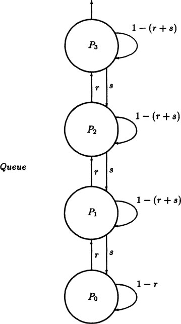
We have, therefore, to think about the state of the queue (its length), and we are in the state diagram area (Section 4.4) with the interesting restriction (usually) that the transitions are only between adjacent states, one more customer arrives or else one more service is completed. And we also face the interesting fact that potentially there are an infinite number of states in the state diagram. Thus for being in state P₀, P₁, P₁, • • • P_k, … (with k items in the queue) we have the corresponding probabilities at time t of $P_0(t),P_1(t),P_2(t),\dots ,P_k(t),\dots$. see Figure 5.10–1.

FIGURE 5.10–1

We now write the transition probability equations. The probability of the queue being in state k at time t + Δt arises from (1) staying in the state, (2) coming from the state k − 1 by another arrival, or (3) coming from state k + 1 by the completion of a service. We neglect the chance of two or more such events in the small time Δt; ultimately we will take the limit as Δt approaches zero, and a double event is a higher order infinitessimal than a single event. We have

$P_k(t+\Delta t)=\{1-(r+s)\Delta t\}{P}_k(t)+\left\{r\Delta t\right\}{P}_{k-1}(t)+\left\{s\Delta t\right\}{P}_{k+1}(t)$

where, of course, the state P_-1 (t) = 0. We have, upon rearrangement,

$\frac{P_k(t+\Delta t)-P_k(t)}{\Delta t}=r{P}_{k-1}(t)-(r+s)P_k(t)+s{P}_{k+1}(t)$

In the limit as Δt → 0 we get the differential equations

$\frac{d{P}_k(t)}{dt}=r{P}_{k-1}(t)-(r+s)P_k(t)+s{P}_{k+1}(t)$

If we start with an empty queue, then the initial conditions are:

$\begin{array}{ccc}{P}_0(0)=1,& P_k(0)=0,& k>0.\end{array}$

To check these differential equations we add them and note that each term on the right occurs with a total coefficient (in the sum) of exactly 0, since the first few equations are clearly

$\begin{array}{cccc}\frac{d{P}_0(t)}{dt}=& & & -r{P}_0(t)+s{P}_1(t)\end{array}$$\begin{array}{ccc}\frac{d{P}_1(t)}{dt}=& & r{P}_0(t)-(r+s)P_1(t)+s{P}_2(t)\end{array}$$\begin{array}{ccc}\frac{d{P}_2(t)}{dt}=& & r{P}_1(t)-(r+s)P_2(t)+s{P}_3(t)\end{array}$$\begin{array}{ccc}\frac{d{P}_3(t)}{dt}=& & r{P}_2(t)-(r+s)P_3(t)+s{P}_4(t)\end{array}$$\begin{array}{cccc}\cdots & \cdots & \cdots & \cdots \end{array}$

Since the sum of the derivatives is zero the sum of the probabilities is a constant, and from the initial conditions this constant is 1; probability is conserved in the queue.

There is a known generating function for the solutions P_k(t) which involves Bessel functions of pure imaginary argument but it is of little use except to get the mean and variance (which, since the Bessel function satisfies a linear second order differential equation, are easy to get from only the first derivative).

What is generally first wanted in queuing problems is the equilibrium solution, the solution that does not involve the exponentials which decay to zero as time approaches infinity. We will not prove that all the eigenvalues of the corresponding infinite matrix have negative real parts, so that they decay to zero, but it is intuitively clear that this must be so (since the probablities are non negative and total up to 1).

The equilibrium solution naturally has the time derivatives all equal to zero—hence at equilibrium we have the infinite system of simultaneous linear algebraic equations on the right hand sides to solve. They are almost triangular and that makes it a reasonable system to solve. We begin by assuming some unknown value for the equilibrium solution value P₀. From the the first equation we get

$P_1=\frac{r}{s}{P}_0$

Using these two values we get from the next equation

$P_2=\frac{1}{s}[(r+s)P_1-r{P}_0]$

and some algebraic simplification gives

$P_2={\left(\frac{r}{s}\right)}^2{P}_0$

It is an easy induction (with P₀ as a basis) to show that

$P_n={\left(\frac{r}{s}\right)}^n{P}_0$

We did not know the value of P₀ with which we started, but merely assumed some value P₀. Using the fact that we know that the sum of all the probabilities must be exactly 1, we have

$1={\displaystyle \sum _{n=0}^{\infty }{P}_n}=P_0{\displaystyle \sum _0^{\infty }{\left(\frac{r}{s}\right)}^n}$

The sum is a geometric progression with a common ratio (r/s) less than 1 so that the series converges). Hence we get

$1=P_0\left[\frac{1}{1-r/s}\right]$

and

$P_0=1-r/s$

Thus the equilibrium solution is

$P_n={\left(\frac{r}{s}\right)}^n(1-r/s)={\left(\frac{r}{s}\right)}^n-{\left(\frac{r}{s}\right)}^{n+1}$

It is necessary to dwell on what this solution means. It does not mean that the queuing system settles down to a set of fixed values—no! The queue continues to change as customers enter the system and have their service completed. The formula means that the probabilities you estimate for the queue length at some distant future time t will settle down to these fixed values. Due to the randomness of the arrivals the actual queue length continues to fluctuate indefinitely. The equilibrium state gives you probability estimates in the long run, but as we said a number of times before what you “expect” to see and what you “actually” see are not the same thing. It is evident, however, that for many purposes the equilibrium solution is likely to be what you want, and you are not interested in the transient of the probability distributions which involves the exponential solution.

We began with a very simple model of a queue, but if we are willing to settle for the equilibrium solution then we are not afraid of much more complex situations. The actual time dependent solutions are not hard to find in this case.

Exercises 5.10

5.10–1 If r = ks(k < 1) compute P_n. Evaluate for k = 1/2 to k = 9/10.

5.10–2 In Exercise 5.10–1 find the generating function of the queue length, and hence the mean and variance.

5.11  Birth and Death Systems

In birth and death systems (the name comes from assuming that items are born and die in various states and when this happens you migrate to the adjacent state, up for birth and down for death) we assume again that in the state diagram only adjacent states are connected, but this time we have that the probability of going to a state depends on the state that you are in, that is r and s are now dependent on the state you are in. In Figure 5.10–1 the transition probabilities from states to states acquire subscripts. By exactly the same reasoning as before we are led this time to the equations

$\frac{d{P}_n(t)}{dt}=r_{n-1}{P}_{n-1}(t)-(r_n+s_n)P_n(t)+s_{n+1}{P}_{n+1}(t)$$\frac{d{P}_0(t)}{dt}=-r_0{P}_0(t)-+s_1{P}_1(t)$

To get the equilibrium solutions we proceed as before; we first put the time derivatives equal to zero, assume a first value for P₀ state, and then solve the equations one at a time. We find

$P_1=\frac{r_0}{s_1}{P}_0$$P_{n+1}=\frac{r_n}{s_{n+1}}{P}_n$

From which we easily find by successive substitutions

$P_n=\frac{r_0{r}_1\cdots r_{n-1}}{s_1{s}_2\cdots s_n}{P}_0$

Our equation for the total probability is now

$1=P_0\left[1+\frac{r_0}{s_1}+\frac{r_0{r}_1}{s_1{s}_2}+\cdots +\frac{r_0{r}_1\cdots r_{n-1}}{s_1{s}_2\cdots s_n}+\cdots \right]$

If and only if this series in the square brackets converges to some finite value S can we get the value of P₀ = 1/S, and hence get all the other values P_n. The divergence of the series implies that there is no equilibrium solution.

We have a general equilibrium solution, and if we want a more compact solution then we have to make some more assumptions (beyond the convergence) on the forms of the r_n and s_n. Whenever you can solve the infinite almost triangular system of algebraic linear equations in a neat form you can get the corresponding neat solution. We will not go into the various cases here as this book is not a course in birth and death processes nor in queuing theory. The purpose is only to show the range of useful problems that fall within the domain of simple probability problems and state diagrams.

Exercises 5.11

5.11–1 Show that for no deaths the solution is $p_n=\exp (-rt){(rt)}^n/n!$

5.12  Summary

We did not lay down postulates and make deductions for the case of continuous probability, rather we proceeded sensibly and from a few simple Examples we saw the kinds of things we might want to assume.

We gave a number of Examples which show that it is non-trivial to decide which, if any, probability distribution to assume is uniform. The assignment of the probability distributions in the continuous case is often a serious problem (that tends to be glossed over in mathematics by making convenient assumptions), and clearly affect the results found after the more formal manipulations. The topic is discussed in much more detail in Chapters 6, 7 and 8.

When the independent variable is time then it is often easy and natural to assign the corresponding probabilities—typically a constant rate in time. Examples are bacterial growth, radioactive decay, failures in electronic systems, and service requirements.