7

Maximum Entropy

“There is no doubt that in the years to come the study of entropy will become a permanent part of probability theory;… ”

A. I. Khinchin (in 1933) [K,p.2]

7.1    What is Entropy?

The main purpose for studying entropy is that it provides a new tool for assigning initial probability distributions. The method is consistant with our symmetry approach but also includes nonuniform distributions. Thus it is a significant extension of the principle of symmetry.

Just as the word “probability” is used in many different senses, the word “entropy” also has several, perhaps incompatible, meanings. We therefore need to examine these different usages closely since they are the source of a great deal of confusion—especially as most people have only a slight idea of what “entropy” means. We will examine four different meanings that are the more common usages of the word. Since this is not a book on thermodynamics or statistical mechanics the treatment must, of necessity, be fairly brief and superficial in the thermodynamically related cases.

The word entropy apparently arose first in classical thermodymanics. Classical thermodynamics treats state variables that pertain to the whole system, such as pressure, volume and temperature of a gas. Besides the directly measurable variables there are a number of internal states that must be inferred, such as entropy and enthalpy. These arise from the imposition of the law of the conservation of energy and describe the internal state of the system. A mathematical equation that arises constantly is

$dH=dQ/T$

where dH is the change (in the sense of engineers and physicists) in entropy, T refers to the absolute temperature, and dQ is the quantity of heat transferred at temperature T. From the assumed second law of thermodynamics (that heat does not flow spontaneously from cold to hot) it is asserted that this quantity can only increase or stay the same through any changes in a closed system. Again, classical thermodynamics refers to global properties of the system and makes no assumptions of the detailed micro structure of the material involve.

Classical statistical mechanics tries to model the detailed structure of the materials, and from this model to predict the rules of classical thermodynamics. This is “micro statistics” in place of “macro statistics” of classical thermodynamics. Crudely speaking, matter is assumed to be little hard, perfectly elastic, balls in constant motion, and this motion of the molecules bouncing against the walls of the container produces the pressure of the gas, for example. Even a small amount of gas will have an enormous number N of particles, and we imagine a phase space whose coordinates are the position and velocity of each particle. This phase space is a subregion of a 6N dimensional space, and in the absence of any possibility of making the requisite measurements, it is assumed that for a fixed energy every small region in the phase space has the same probability as any other (compare the Poincare theory of small causes, large effects). Then average values over the phase space are computed. Boltzmann broke up the phase space into a large number of very small regions and found that the quantity

$H=k\log \frac{1}{P}$

seemed to play a role similar to the classical concept of entropy (k is Boltz-mann’s constant and P is the probability associated with any one of the equally likely small regions in the phase space with the given energy.

Boltzmann attempted to prove the famous Boltzmann’s “H theorem” which states that with increasing time H could not decrease but would generally increase. It was immediately pointed out by Loschmidt that since Boltzmann began with Newtonian mechanics, in which all the equations of motion that he used are reversible, then it is impossible from this aione to deduce irreversibility. A lot of words have been said about the probabilities of the states when all the velocities of the particles are reversed (to make things go backwards in time), and it is usually claimed that these states are much less likely to occur than those in the original direction—though so far as the author knows there never has been any careful mathematical proof, only the argument that this must be so in order for the theorem they wanted to be true! Kac gave an interesting simple counter example to the proof using only a finite system that was clearly periodic and reversible. (See Wa, pp.396–404)

This, then, is the second entropy that is widely used, and is thought to be connected with the “mixed-up-ness” of the system.

Gibbs, in trying to deal with systems which did not have a fixed energy introduced the “grand cannonical ensemble” which is really an ensemble of the phase spaces of different energies of Boltzmann. In this situation he deduced an entropy having the form

$H={\displaystyle \sum _{i}p(i)\mathit{ln}\frac{1}{p(i)}}$

where the p(i) are the probabilites of the phase space ensembles. This, then, is still a third kind of physical entropy.

Shannon while creating information theory found an expression of exactly the same form, and called it entropy, apparently on the advice of von Neumann, (“You should call it ‘entropy’ for two reasons: first, the function is already in use in thermodynamics under that name; second, and more importantly, most people don’t know what entropy really is, and if you use the word ‘entropy’ in an argument you will win every time!”) [L-T, p.2]

But the identity of mathematical form does not imply identity of meaning. For example, Galileo found that falling bodies obey the formula

$s=\frac{g}{2}{t}^2$

and Einstein found the famous equation

$E=m{c}^2$

but few people believe that the two equations have much in common except that both are parabolas. As the derivation of Shannon’s entropy in the next section will show, the variables in his equation bear little resemblence to those of Gibbs or Boltzmann. However, from Shannon’s entropy Tribus has derived all the basic laws of thermodynamics [L-T] (and has been ignored by most thermodynamicists).

While the identity of form cannot prove the identity of meaning of the symbols, it does mean that the same formal mathematics can be used in both areas. Hence we can use many of the formal mathematical results and methods, but we must be careful in the interpretations of the results.

7.2    Shannon’s Entropy

Let X be a discrete random variable with probabilities p(i), (i = 1,2,…, n). We shall show in a few moments that when dealing with “information” the standard assignment for the amount of information, I{p(i)}, to be associated with an outcome of probability p(i), is measured by the “surprise,” the likelihood of the event, or the information gained, which is

$I\{p(i)\}=\log \frac{1}{p(i)}=-\log p(i)$

In the certain event p = 1, and no new information is obtained when it happens.

The result of this assignment is that the expected value of the information I(X) for a random variable X is given by the formula,

$H(X)=E\{I(X)\}={\displaystyle \sum _{i=1}^{n}p(i)\log \frac{1}{p(i)}}$

(7.2–1)

In information theory this is called the entropy. It is usually labeled H(X), or sometimes H(p).

Information theory usually uses the base 2 for the logarithm system, which we do in this chapter unless the contrary is explicitly stated. Logs to the base e will be denoted, as usual, by ln.

Kullback [Ku] has written a book (1959) with the title, Information Theory and Statistics, which shows many of the connections between the two fields.

This assignment of values to a random variable X is one of a number of different intrinsic assignments of values to the outcomes of a trial of a random variable, “intrinsic” meaning that the values come directly from the probabilities and have no extrinsic source. The general case of intrinsic assignments is the assignment of the value of the random variable as some function f(p(i)). In contrast, dealing with the time to first failure for a run of n trials gives an extrinsic but natural assignment of the index n as the values for the possible outcomes of probabilities qp^n-1, (n = 1,2,…).

The entropy can also be viewed in a different way; since

$p(i)\log \frac{1}{p(i)}=\log {\left\{\frac{1}{p(i)}\right\}}^{p(i)}$

we have

$H(X)=-\log {\displaystyle \prod _{i=1}^{n}p{(i)}^{p(i)}}$

and taking antilogs of both sides we have

$2^{-H(X)}={\displaystyle \prod _{i=1}^{n}p{(i)}^{p(i)}}$

(7.2–2)

which resembles a weighted geometric mean of the probabilities. Because of this logarithmic structure Shannon’s entropy has many of the properties of both the arithmetic and geometric means.

Example 7.2–1    An Entropy Computation

Given a random variable X with the probability distribution p(1) = 1/2, p(2) = 1/4, p(3) = 1/8, and p(4) = 1/8, the entropy of the distribution is

$\begin{array}{c}H(X)=(1/2)\log 2+(1/4)\log 4+(1/8)\log 8+(1/8)\log 8\\ =(1/2)(1)+(1/4)(2)+(1/8)(3)+(1/8)(3)\\ =1/2+1/2+3/8+3/8=7/4\end{array}$

From any finite probability distribution we obtain the entropy as a single number—much as the mean is a single number derived from a distribution.

The entropy function measures the amount of information contained in the distribution, and is sometimes called the negentropy since it is thought to be the negative of the usual entropy which in turn is supposed to measure the “mixed-up-ness” of a distribution. We have already exposed the weakness of the analogy of Shannon’s entropy with the entropies of physics, but see [T],[L-T]. For biology see [Ga].

Since we will be using Shannon’s entropy extensively we need to make some reasonable derivation of his entropy function. Let there be two independent random variables X and Y with outcomes x_i and (say the roll of a die and the toss of a coin). How much information is contained in the observed outcome x_iy_j? If I(.) is the measure of the amount of information then we believe that for independent random variables the total information is the sum of the information contained in the individual outcomes, that is

$I(x_i{y}_j)=I(x_i)+I(y_j)$

(7.2–3)

Think this over carefully before accepting it as fitting your views of information.

Equation (7.2–3) is the standard Cauchy functional equation when we also suppose that the measure of information I(p) is a non-negative continuous function of its argument.

To study the solution of Cauchy’s equation we drop the subscripts. Consider the functional equation (defines a function rather than a number)

$f(xy)=f(x)+f(y)$

(7.2–4)

where f(x) is a continuous nonnegative function of x. Suppose that y = x, then we have from equation (7.2–4)

$f(x^2)=2f(x)$

Next, let y = x². Then from equation (7.2–4) we get

$f(x^3)=3f(x)$

and in general, by induction, we have for all integers n > 0,

$f(x^n)=nf(x)$

Now if we write xⁿ = z we have

$f(z)=nf(z^{1/n})$

or rewriting this

$f(z^{1/n})=(1/n)f(z)$

Proceeding as before, we can show that for all rational numbers p/q

$f(z^{p/q})=(p/q)f(z)$

By the continuity assumption on the solution of the equation since the equality holds for all rational numbers it holds for all real numbers, x > 0 and y

$f(x^y)=yf(x)$

(7.2–5)

The relationship (7.2–5) suggests that the solution is f(x) = logx to some base. To prove that this solution is unique to within a constant multiplier (effectively the base chosen for the logs) we assume that there is a second solution g(x), and then consider the difference

$f(x)-kg(x)={\log }_{2}x-kg(x)$

where, of course from (7.2–5) g(x^y) = yg(x). We have for the difference

$\log x-kg(x)=(1/y)\{\log x^y-kg(x^y)\}$

We fix in our minds some x = x₀, (not 0 or 1), and choose a particular k so that at x = x₀ the left hand side is zero (so that the scaled second solution has a common point with the log solution at x = x₀). Hence we set

$k=\frac{\log x_0}{g(x_0)}$

We have on the right

$\log x_0^y-kg(x_0^y)=0$

Now for any z other than 0 and 1 there is a y such that

$\begin{array}{ccc}z=x_0^y& \text{namely}& y=\frac{\log z}{\log x_0}\end{array}$

and we have

$\log z=kg(z)=g(z)\frac{\log x_0}{g(x_0)}$

Therefore any other solution g(z) is proportional the log z; and the solutions differ only with respect to the logarithm base used.

It is conventional to use, in information theory, the base 2 so that a simple binary choice has unit information; it is only a difference in the units used to measure information that is being determined by the choice of base 2. The standard equation

$\log x=\frac{{\log }_{b}x}{{\log }_{b}2}=({\log }_{2}b)({\log }_{b}x)$

means that every log system is proportional to every other, and the conversion from one to another is simple.

Since by assumption I(p) ≥ 0 it is necessary to use a negative value for k so we finally choose our solution of equation (7.2–3) as

$I(p)=\log \frac{1}{p}=-\log p$

(7.2–6)

Now that we have the measure of information for any outcome of probability p, we examine it to see its reasonableness. The less likely the event is to happen the more the information, the more the surprise, the greater the reduction in uncertainty. The certain event p = 1 has no information, while the impossible event has infinite information, but it never occurs! See below, equation (7.2–8).

The average information contained in a distribution p(i) is clearly the weighted average of log{1/p(i)} (the expected value). From (7.2–6) we have

$\begin{array}{c}H(X)={\displaystyle \sum _{i=1}^{n}p(i)\log \frac{1}{p(i)}}\\ =-{\displaystyle \sum _{i=1}^{n}p(i)\log p(i)}\end{array}$

(7.2–7)

which is the entropy of the distribution. The entropy is measured in units of bits per trial.

When we have a binary choice then we often write the argument as P (or q)

$H(p)=p\log \frac{1}{p}+q\log \frac{1}{q}=H(q)$

as as matter of convenience since the entropy then depends on the single number p (or q).

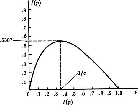
We need to examine the shape (graph) of the typical term of the entropy function as a function of the probability p. There is clearly trouble at p = 0. To evaluate this indeterminate form we first shift to logs to the base e and later rescale.

$\underset{p\to 0}{\lim }p\mathit{ln}\frac{1}{p}=\underset{p\to 0}{\lim }\left[\frac{\mathit{ln}(1/p)}{1/p}\right]$

We can now apply l’Hopital’s rule,

$\underset{p\to 0}{\lim }\left[\frac{-1/p}{-1/p^2}\right]=\underset{p\to 0}{\lim }p=0$

(7.2–8)

and we see that at p = 0 the term pln(1/p) = 0. Thus while the impossible event has infinite information the limit as p approaches 0 of the probability of its occurrence multiplied by the amount of information is still 0. We also see that the entropy of a distribution with one p(i)= 1 is 0; the outcome is certain and there is no information gained.

FIGURE 7.2–1

For the slope of the curve y = pln(1/p) we have

$y^{\prime }=-1-\mathit{ln}p$

and it is infinite at p = 0. The maximum of the curve occurs at p = 1/e. Thus, rescaling to get to logs base 2, we have the Figure 7.2–1.

In coding theory it can be shown that the entropy of a distribution provides the lower bound on the average length of any possible encoding of a uniquely decodable code for which one symbol goes into one symbol. It also arises in an important binomial coefficient inequality

${\displaystyle \sum _{k=0}^{an}C(n,k)\le 2^{nH(a)}}$

(7.2–9)

where a < 1/2 and provided n is made sufficiently large. Thus the entropy function plays an important role in both information theory and coding theory.

Example 7.2–2    The Entropy of Uniform Distributions

How much information (on the average) is obtained from the roll of a die? The entropy is

$\begin{array}{ll}H(X)\hfill & ={\displaystyle \sum _{i=1}^6\frac{1}{6}\log 6}\hfill \\ \hfill & =\log 6=2.584962\dots \text{bits/roll}\hfill \end{array}$

Similarly, for any uniform choice from n things the entropy is

$\begin{array}{cc}H(X)=\log n& \text{bits/trial}\end{array}$

which gives a reasonable answer. In the cases where n = 2^k you get exactly k bits of information per trial.

Exercises 7.2

7.2–1 Show that (7.2–9) holds at a = 1/2.

7.2–2 Compute the entropy of the distribution p(i) = 1/8, (i = 1,2,…, 8).

7.2–3 Compute the entropy of p(i) = 1/3, 1/3, 1/9, 1/9, 1/9.

7.2–4 Show that ${\displaystyle {\int }_0^{1}I(p)dp=0.3606\dots }$.

7.2–5 For the probabilities 1/3, 1/4, 1/6, 1/9, 1/12, 1/18 show that the entropy is 8/9 + (11/12) log 3 ~ 2.34177.

7.2–6 Let $S_N={\displaystyle {\sum }_{n=1}^{N}1/n}$. Then Zipf’s distribution has the probabilities $p_n=(1/n)/S_N$. If $T_N={\displaystyle {\sum }_{n=1}^N(\log n)/n}$ show that the entropy of Zipf’s distribution is $H(N)=T_N/S_N+\log S_N$.

7.2–7 Using Appendix A.l estimate the entropy of Zipf’s distribution.

7.3    Some Mathematical Properties of the Entropy Function

We now investigate this entropy function of a distribution as a mathematical function independent of any meaning that may be assigned to the variables.

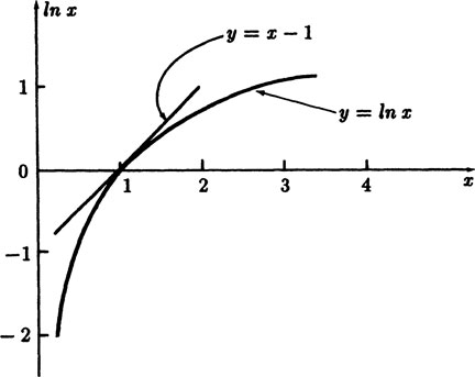
Example 7.3–1    The log Inequality

The first result we need is the inequality

$\mathit{ln}x\le 1-x$

(7.3–1)

This is easily seen from Figure 7.3–1 where we fit the tangent line to the curve at x = 1. The derivative of ln x is 1/x, and at x = 1 the slope is 1. The tangent line at the point (1,0) is

FIGURE 7.3–1

$y-0=1(x-1)$

or

$y=x-1$

Since y = ln x is convex downward (y” = −1/x² < 0) the inequality holds for all values of x > 0, and the equality holds only at x = 1. Compare with Appendix 1.B.

Example 7.3–2    Gibbs’ Inequality

We now consider two random variables X and Y with finite distributions px(i) and py(i), both distributions with the sum of their values equal to 1. Starting with (using natural logs again)

${\displaystyle \sum _{i=1}^n{p}_X(i)\mathit{ln}\frac{p_Y(i)}{p_X(i)}}$

we apply the log inequality (7.3–1) to each log term to get

$\begin{array}{ll}{\displaystyle \sum _{i=1}^n{p}_X(i)\mathit{ln}\frac{p_Y(i)}{p_X(i)}}\hfill & \le {\displaystyle \sum _{i=1}^n{p}_X(i)\left\{1-\frac{p_Y(i)}{p_X(i)}\right\}}\hfill \\ \hfill & \le {\displaystyle \sum _{i=1}^n{p}_X(i)}-{\displaystyle \sum _{i=1}^n{p}_Y(i)=1-1=0}\hfill \end{array}$

The equality holds only when each p_X(i) = p_Y (i). Since the right hand side is 0 we can multiply by any positive constant we want and thus, if we wish, convert to base 2. This is the important Gibbs’ inequality

${\displaystyle \sum _{i=1}^n{p}_X(i)\log \frac{p_Y(i)}{p_X(i)}\le 0}$

(7.3–2)

The equality holds only when p_X(i) = p_Y (i) for all i.

Example 7.3–3    The Entropy of Independent Random Variables

Suppose we have two independent random variables X and Y and ask for the entropy of their product. We have

$\begin{array}{c}H(XY)={\displaystyle \sum _i^j{p}_X(x_i)p_Y(y_j)\log \frac{1}{p_X(x_i)p_Y(y_j)}}\\ ={\displaystyle \sum _i^j{p}_X(x_i)p_Y(y_j)\log \frac{1}{p_X(x_i)}+\log \frac{1}{p_Y(y_j)}}\end{array}$

When we sum over the variable not in the log term we get a factor of 1, and when we sum over the variable in the log term we get the corresponding entropy; hence

$H(XY)=H(X)+H(Y)$

(7.3–3)

When we compare this with (2.5–4)

$E\{X+Y\}=E\left\{X\right\}+E\left\{Y\right\}$

we see that the entropy of the product of independent random variables satisfies the same equation as the expectation on sums (independent or not), and partly explains the usefulness of the entropy function.

Suppose next that we have n independent random variables X_i, (i = 1,…, n), and consider the entropy of the compound event S = X₁X₂ … X_n. We have, by similar reasoning,

$H(S)=H(X_1)+H(X_2)+\cdots +H(X_n)$

(7.3–4)

Thus n repeated trials of the same event X gives the entropy

$H(S)=nH(X)$

(7.3–5)

This is what one would expect when you examine the original definition of information carefully.

Example 7.3–4    The Entropy Decreases When You Combine Items

We want to prove that if we combine any two items of a distribution then the entropy decreases, that we lose information. Let the two items have probabilities p(i) and p(j). Since probabilities are non-negative it follows that

$p(i)\le p(i)+p(j)$

$\log p(i)\le \log \{p(i)+p(j)\}$

$\log 1/p(i)\ge \log \frac{1}{p(i)+p(j)}$

Now: (1) multiply the last equation by p(i), (2) interchange i and j, and (3) add the two equations to get

$p(i)\log \frac{1}{p(i)}+p(j)\log \frac{1}{p(j)}\ge \{p(i)+p(j)\}\log \frac{1}{p(i)+p(j)}$

and we have our result which agrees with our understanding of Shannon’s entropy: combining items loses information.

Exercises 7.3

7.3–1 What is the amount of information in drawing a card from a deck? Ans. log 52 = 5.7004397 … bits/draw.

7.3–2 What is the amount of information in drawing k cards without replacement from a deck?

7.3–3 Compute the entropy of the distribution p₁ = 1/2, p₂ = 1/4, p₃ = 1/8, p₄ = 1/16, p₅ = 1/16.

7.3–4 Write a symmetric form of Gibbs’ inequality.

7.3–5 Show that when combining two items having the same probability p(i) you lose –2p (i) ln 2 of information.

7.3–6 If you have a uniform distribution of 2n items and combine adjacent terms thus halving the number of items, what is the information loss?

7.3–7 What is the information in the toss of a coin and the roll of a die?

7.3–8 What is the information from the roll of n independent dice?

7.3–9 Show that the information from the toss of n independent coins = n.

7.4    Some Simple Applications

We now show that Shannon’s definition of entropy has a number of other reasonable consequences that justify our special attention to this function.

Example 7.4–1    Maximum Entropy Distributions

We want to show that the distribution with the maximum entropy is the flat distribution. We start with Gibbs’ inequality, and assign the p_Y(i) = 1/n (where n is the number of items in the distribution). We have

${\displaystyle \sum _i{p}_X(i)\log \frac{1}{n{p}_X(i)}\le 0}$

Write the log term of the product as the sum of logs and transpose the terms in n. We have

$H(X)={\displaystyle \sum _i{p}_X(i)\log \frac{1}{p_X(i)}}\le {\displaystyle \sum _i{p}_X(i)\log n=\log n}$

or

$H(X)\le \log n$

and we know that the Gibbs equality will hold when and only when all the p_X(i) are equal to the p_Y(i), that is p_X(i) = 1/n, which is the uniform distribution. When the entropy is maximum then the distribution is uniform and

$\max \{H(X)\}=\log n$

(7.4–1)

This includes the converse of Example 7.2–2.

For a finite discrete uniform distribution the entropy is a maximum; and conversely if the entropy is maximum the distribution is uniform. This provides some further justification for the rule that in the absence of any other information you assign a uniform probability (for discrete finite distributions). Any other finite distribution assumes some constraints, hence the uniform distribution is the most unconstrained finite distribution possible. See Chapter 6.

This definition of the measure of information agrees with our intuition when we are in situations typical of computers and the transmission of information as in the telephone, radio, and TV. But it also says that the book (of a given size and type font) with the most information is the book in which the symbols are chosen uniformly at random! Each symbol comes as a complete surprise.

Randomness is not what humans mean by information. The difficulty is that the technical definition of the measure of information is connected with surprise, and this in no way involves the human attitude that information involves meaning. The formal theory of information avoids the “meaning” of the symbols and only considers the “surprise” at the arrival of the symbol, thus you need to be wary of applying information theory to situations until you are sure that “meaning” is not involved. Shannon was originally urged to call it communication theory but he chose information theory instead.

A second fault is that the definition is actually a relative definition—relative to the state of your knowledge. For example, if you are looking at a source of random numbers and compute the entropy you get one result, but if I tell you the numbers are from a particular pseudo random number generator then they are easily computed by you and contain no surprise, hence the entropy is 0. Thus the entropy you assign to a source depends on your state of knowledge about it—there is no meaning to the words “the entropy of a source” as such!

Example 7.4–2    The Entropy of a Single Binary Choice

It very often happens that you face a binary choice, yes-no, good-bad, accept-reject, etc. What is the entropy for this common situation? We suppose that the probability of the first one is p, and hence the alternate is q = 1 − p. The entropy is then

$H(p)=p\log \frac{1}{p}+q\log \frac{1}{q}=H(q)$

where again we use the probability p as the argument of H since there is only one value to be given; for the general distribution we must, of course, give the whole distribution (minus, if you wish, one value due to the sum of all the p(i) being 1), and hence we generally use the name X of the random variable as the argument of H(X).

Example 7.4–3    The Entropy of Repeated Binary Trials

Suppose we have a repeated binary trial with outcome probabilites p and q, and consider strings of n trials. The typical string has the probability

$ppqqpqp\dots pqq=p^k{q}^{n-k}$

and for each k there are exactly C(n, k) different strings with the same probability. We have, therefore, that the entropy of the distribution of repeated trials is

$H={\displaystyle \sum C(n,k)p^k{q}^{n-k}\log \frac{1}{p^k{q}^{n-k}}}$

We could work this out directly in algebraic detail and get the result, but we know in advance, from the result (7.3–5), that it will be (in the binary choice we can and do use just p as the distribution)

$H=nH(p)=nH(q)=n\left[p\log \frac{1}{p}+q\log \frac{1}{q}\right]$

(7.4–2)

We may define a conditional entropy when the events are not independent. Consider two related random variables X and Y. We have, dropping indices since they are obvious,

$p(x,y)=p(x)p(y|x)$

Thinking of the distribution p(y|x) for a fixed x we have

$H(Y|x)={\displaystyle \sum _{y}p(y|x)\log \frac{1}{p(y|x)}}$

as the conditional entropy of y given x. If we multiply these conditional entropies by their respective probabilities of occurance p(x) we get

$\begin{array}{ll}H(Y|X)\hfill & ={\displaystyle \sum p(x)p(y|x)\log \frac{1}{p(y|x)}}\hfill \\ \hfill & ={\displaystyle \sum p(x,y)\log \frac{1}{p(y|x)}}\hfill \end{array}$

Thus entropies may be computed in many ways and are a flexible tool in dealing with probability distributions.

The entropy is the mean of {– logp(i)}; what about the variance of the distribution? We have easily

$\text{Var}=E\left\{{\left[\log \frac{1}{p(i)}-H\right]}^2\right\}=E\{{\log }^{2}p(i)\}-H^2$

(7.4–3)

Example 7.4–4    The Entropy of the Time to First Failure

The time to the first failure is the random variable (p = probability of success)

$\begin{array}{cc}X=\left\{p^{n-1}q\right\}& (n=1,2,\dots )\end{array}$

If we compute the entropy we find

$H(X)={\displaystyle \sum _{n=1}^{\infty }{p}^{n-1}q\log \frac{1}{p^{n-1}q}}$

Shifting the summation index by 1 we get (using equations (4.1–2) and (4.1–4))

$\begin{array}{ll}H(X)\hfill & =q{\displaystyle \sum _{n=0}^{\infty }{p}^n\left\{\log \frac{1}{q}+n\log \frac{1}{p}\right\}}\hfill \\ \hfill & =q\log \frac{1}{q}{\displaystyle \sum _{n=0}^{\infty }{p}^n+q\log \frac{1}{p}}{\displaystyle \sum _{n=0}^{\infty }n{p}^n}\hfill \\ \hfill & =q\log \frac{1}{q}\left\{\frac{1}{1-p}\right\}+q\log \frac{1}{p}\left\{\frac{p}{{(1-p)}^2}\right\}\hfill \\ \hfill & =\log \frac{1}{q}+\frac{p}{q}\log \frac{1}{p}=\frac{1}{q}H(p)\hfill \end{array}$

(7.4–4)

The above results depend on being a discrete countably infinite distribution. But for some discrete infinite distributions the entropy does not exist (is infinite). We need to prove this disturbing property. Because of the known theorem that for monotone functions the improper integral and infinite series converge and diverge together, we first examine the improper integrals (using log_e = ln)

${{\displaystyle {\int }_2^{\infty }\frac{1}{x\mathit{ln}x}dx=\mathit{ln}\mathit{ln}x}|}_2^{\infty }\to \infty$

${{\displaystyle {\int }_2^{\infty }\frac{1}{x{\mathit{ln}}^{2}x}dx=\frac{-1}{\mathit{ln}x}}|}_2^{\infty }=\frac{1}{\mathit{ln}2}$

From these we see that

${\displaystyle \sum _2^{\infty }\frac{1}{n\log n}\to \infty }$

(7.4–5)

$\begin{array}{cc}{\displaystyle \sum _2^{\infty }\frac{1}{n{\log }^{2}n}=A}& (\text{a finite number)}\text{.}\end{array}$

We use these results in the following Example.

Example 7.4–5    A Discrete Distribution with Infinite Entropy

The probability distribution X with

$\begin{array}{cc}p(n)=\frac{1}{A(n{\log }^{2}n)}& (n=2,3,\dots )\end{array}$

has a total probability of 1 (from the above equation (7.4–5) A > 0). But the entropy of X is

$\begin{array}{ll}H(X)\hfill & ={\displaystyle \sum _{n=2}^{\infty }p(n)\log \frac{1}{p(n)}}\hfill \\ \hfill & ={\displaystyle \sum _{n=2}^{\infty }p(n)\log \left\{An{\log }^{2}n\right\}}\hfill \\ \hfill & =\frac{1}{A}{\displaystyle \sum _2^{\infty }\frac{1}{n{\log }^{2}n}\{\log A+\log n+2\log \log n\}}\hfill \\ \hfill & =\frac{1}{A}{\displaystyle \sum _2^{\infty }\left\{\frac{\log A}{n{\log }^{2}n}+\frac{1}{n\log n}+\frac{2\log \log n}{n{\log }^{2}n}\right\}}\hfill \end{array}$

The first term converges; the second term diverges; and the third term is positive so there is no possibility of cancellation of the infinity from the second term—the entropy is infinite.

Thus there are discrete probability distributions which have no finite entropy. True, the distributions are slowly convergent and the entropy slowly diverges, but it is a problem that casts some doubt on the widespread use of the entropy function without some careful considerations. We could, of course, by fiat, exclude all such distributions, but it would be concealing a basic feature that the entropy of discrete probability distributions with an infinite number of terms can be infinite. Similar results apply to continuous distributions, either for infinite ranges or for a finite range and infinite values in the interval (use for example the simple reciprocal transformation of variables).

Exercises 7.4

7.4–1 Plot H(p).

7.4–2 Complete the detailed derivation of the entropy of the binomial distribution.

7.4–3 What is the entropy of the distribution $p(n)=A^{\prime }/n^{3/2}$?

7.4–4 Find the entropy of the distribution $p(n)=(1-a)a^n,n=0,1,2,\dots$.

7.5    The Maximum Entropy Principle

The maximum entropy principle states that when there is not enough information to determine the whole probability distribution then you should pick the distribution which maximizes the entropy (compatible with the known information, of course).

In a sense the maximum entropy principle is an extension of the principle of indifference, or of consistency (see Section 6.4), since with nothing known both principles assign a uniform distribution (Example 7.4–1). When some facts are known they are first used, and then the principle of maximum entropy is invoked to determine the rest of the details of the distribution. Again (see the next Example), the result is reasonable, and the independence is usually regarded as less restrictive than the assumption of some correlations in the table. Thus the maximum entropy assumes as much independence as can be obtained subject to the given restrictions.

Example 7.5–1    Marginal Distributions

Suppose we have a distribution of probabilities p(i, j) depending on two indices of ranges m and n. We are often given (or can measure) only the marginal distributions, which are simply the row sums R(i)

$\begin{array}{ccc}{\displaystyle \sum _{j}p(i,j)=R(i)}& \text{with}& {\displaystyle \sum _{i}R(i)=1}\end{array}$

and the column sums C(j)

$\begin{array}{ccc}{\displaystyle \sum _{i}p(i,j)]=C(j)}& \text{with}& {\displaystyle \sum _{j}C(j)=1}\end{array}$

where, of course, the indicated arguments i and j may have different ranges. Thus we have (m + n − 2) independent numbers (satisfying the restrictions on the row and column sums), and wish to assign reasonable values to the whole array p(i,j) consisting of mn- 1 values, (restricted by ${\displaystyle {\sum }_{i,j}p(i,j)=1}$. There is, of course, no unique answer to such situations for m, n > 1.

The maximum entropy rule asserts that it is reasonable to assign the values to the p(i,j), subject to the known restraints, so that the total entropy is maximum. We begin with Gibbs’ inequality

${\displaystyle \sum _i^{j}p(i,j)\log \frac{R(i)C(j)}{p(i,j)}\le 0}$

By the Gibbs’ inequality the entropy is a maximum when all the

$p(i,j)=R(i)C(j)$

(7.5–1)

This is the same thing as assuming that the probabilities in i and j are independent—the least assumption in a certain sense!

We now look as a classic example due to Jaynes [J]. It has caused great controversy mainly because people cannot read what is being stated but only what they want to read, (and Jaynes tends to be belligerent).

Example 7.5–2    Jayne’s Example

Suppose the sample space has six points with values 1,2, …, 6. We are given the information that the average (expected value) is not 7/2 (as it would be if the probabilities were all 1/6) but rather it is 9/2. Thus we have the condition

$E\left\{X\right\}={\displaystyle \sum _{i=1}^{6}ip(i)=9/2}$

(7.5–2)

The maximum entropy principle states that we are to maximize the entropy of the distribution

$E\left\{X\right\}={\displaystyle \sum _{i=1}^{6}p(i)\log \frac{1}{p(i)}}$

subject to the two restrictions: (1) that the sum of the probabilities is exactly 1,

${\displaystyle \sum _{i=1}^{6}p(i)=1}$

(7.5–3)

and (2) that (7.5–2) holds.

We use Lagrange multipliers and set up the function

$L\{p(i)\}=H\left\{X\right\}-\lambda {\displaystyle \sum _{i=1}^6\{p(i)=1\}}-\mu {\displaystyle \sum _{i=1}^6\{ip(i)-9/2\}}$

(7.5–4)

We next find the partial derivatives of L{p(i)} with respect to each unknown p(i), and set each equal to zero,

$\begin{array}{cc}-1-\log p(i)-\lambda -\mu i=0& (i=1,\dots ,6)\end{array}$

(7.5–5)

This set of equations (7.5–5) together with the two side conditions (7.5–2) and (7.5–3) determine the result. To solve them we first rewrite (7.5–5)

$\log p(i)=-(1+\lambda +\mu i)$

(7.5–6)

$p(i)=e^{-(1+\lambda +\mu i)}$

To simplify notation we set

$\begin{array}{cc}{e}^{(1+\lambda )}=A,& e^{-\mu }=x,\end{array}$

(7.5–7)

In this notation the three equations (7.5–6), (7.5–3) and (7.5–2) become

$p(i)=\frac{1}{A}{x}^i$

(7.5–8)

${\displaystyle \sum _{i=1}^6{x}^i=A}$

(7.5–9)

${\displaystyle \sum _{i=1}^{6}i{x}^i=\frac{9}{2}A}$

(7.5–10)

To eliminate A divide equation (7.5–10) by equation (7.5–9)

$\frac{9}{2}=\frac{{\displaystyle \sum _{i=1}^{6}i{x}^i}}{{\displaystyle \sum _{i=1}^6{x}^i}}$

The solution x = 0 is impossible, and we easily get

${\displaystyle \sum _{i=1}^6\left(\frac{9}{2}-i\right)x^{i-1}=0}$

(7.5–11)

Expanding the summation and clearing of fractions we get the following algebraic equation of degree 5 in x,

$3x^5+x^4-x^3-3x^2-5x-7=0$

(7.5–12)

There is one change in sign and hence one positive root which is easily found by the bisection method (or any other root finding method you like). From equation (7.5–9) we get A, and from equation (7.5–8) we get the geometric progression of probabilities p(i) as follows.

$p(1)=0.05435$

$p(2)=0.07877$

$p(3)=0.11416$

$p(4)=0.16545$

$p(5)=0.23977$

$p(6)=0.34749$

Is the result reasonable? The uniform distribution p(k)= 1/6 = 0.16666 has a mean 7/2 that is too low; this distribution has the right mean of 9/2.

To partially check the result we alter the 9/2 to 7/2 where we know the solution is the uniform distribution. The equation (7.5–11) becomes

${\displaystyle \sum _{i=1}^6\left(\frac{7}{2}-i\right)x^{i-1}=0}$

and this upon expanding and multiplying by 2 is (compare with equation (7.5–12))

$5x^5+3x^4+x^3-x^2-3x-5=0$

which clearly has the single positive root x = 1. From equation (7.5–9) A = 6 and from equation (7.5–8) p(i)= 1/6 as we expect.

When we examine the process we see that the definition for A arose as “the normalizing factor” to get from the xⁱ values to the probability values p(i), and it arose from the combination of the entropy function definition plus the condition that the sum of the probabilities is 1. Since these occur in most problems that use the maximum entropy criterion for assigning the probability distribution, we can expect that it will be a standard feature of the method of solution. The root x, see equation (7.5–7), arose from the condition on the mean; other side conditions on the distribution will give rise to other corresponding simplifying definitions. But so long as the side conditions are linear in the probabilities (as are the moments for example), we can expect similar methods to work.

If you do not like the geometric progression of probabilities that is the answer (from the use of the maximum entropy principle) then with nothing else given what other distribution would you like to choose? And how would you seriously defend it?

Example 7.5–3    Extensions of Jaynes’ Example

In order to understand results we have just found, it wise to generalize, to extend, and otherwise explore the Example 7.5–2. We first try not 6 but N states, and assign the mean M. Corresponding to (7.5–2) we have

${\displaystyle \sum _{i=1}^{N}ip(i)=M}$

and in (7.5–4) we have, obviously M in place of 9/2. The set of equations (7.5–5) are the same except there are now n of them. The change in notation equation (7.5–7) is the same. The corresponding three equations are now

${\displaystyle \sum _{i=1}^N{x}^i=A}$

${\displaystyle \sum _{i=1}^{N}i{x}^i=MA}$

$p(i)=\frac{1}{A}{x}^i$

The elimination of A gives corresponding to equation (7.5–11)

${\displaystyle \sum _{i=1}^N(M-i)x^{i-1}=0}$

Again there is one positive root. (The root = 1 only if M is (1 + 2+ … + N)/N = (N + 1)/2. The rest is the same as before.

Another extension worth looking at is the inclusion of another condition on the sum (the second moment)

${\displaystyle \sum _{i=1}^N{i}^{2}p(i)=S}$

We will get the Lagrange equation

$L\{p(i)\}=H(S)-\lambda {\displaystyle \sum _{i=1}^N\{p(i)-1\}}-\mu {\displaystyle \sum _{i=1}^N\{ip(i)-M\}}-\nu {\displaystyle \sum _{i=1}^N\{i^{2}p(i)-S\}}$

The resulting equations are

$\log p(i)=-(1+\lambda +\mu i+\nu i^2)$

The same substitutions (7.5–7) together with e^-v = y give us

${\displaystyle \sum _i{x}^i{y}^{i^2}=A}$

${\displaystyle \sum _{i}i{x}^i{y}^{i^2}=MA}$

${\displaystyle \sum _i{i}^2{x}^i{y}^{i^2}=SA}$

We eliminate A by dividing the second and third equations by the first equation, and we have a pair of equations

${\displaystyle \sum _i(M-i)x^i{y}^{i^2}=0}$

${\displaystyle \sum _i(S-i)x^i{y}^{i^2}=0}$

To solve this pair of nonlinear equations we resort to a device [H, p.97] that is useful. Call the first expression F(x, y) and the second G(x, y). We want a common solution of F = 0 and G = 0. Now for each pair of numbers {x, y) there is a pair of numbers {F(x,y), G(x,y)} and this point falls in some quadrant. Plot in the x-y plane the corresponding quadrant numbers of the point (F, G). The solution we want is clearly where in the F, G variables the four quadrants meet. Thus a crude plot of the quadrant values will indicate this point. A refined plot at a closer spacing in the x-y variables will give a more accurate estimate of the solution. Successive refinements will lead you to as an accurate solution as you can compute. It is not necessary to plot a large region of the x-y plane, you only need to track one of the edges dividing the quadrants, either F = 0 or G = 0, until you meet the other edge dividing the quadrants.

7.6    Summary

In all probability problems there is always the fundamental problem of the initial probability assignment. In the earlier chapters we generally assumed, from symmetry, that the distribution was uniform, but there are times when we need to do something else since the uniform distribuition may not be compatible with the given facts—such as in the above Example 7.5–2 where the mean is 9/2. The maximum entropy principle allows us to make an assignment of the probabilities that in a reasonable sense makes the least additional assumptions about the interrelationships of the probabilities.

That the principle is sometimes useful does not make it the correct one to use in all cases. Nor should the name “entropy” imply any overtones of physical reality. You need to review in your own mind how we got here, what the principle seems to imply, and consider what other principles you might try. That in maximum entropy problems the initial distribution is not completely given is actually no different than when we invoked the principle of indifference (the principle of consistency) to get from no probabilities assigned to the uniform distribution. In those cases where not enough information is given to determine all the details of the initial distribution then something must be assumed to get it. To assert that nothing can be done is not likely to be satisfactory. Nor is the statement that you can get almost anything you want. Sensible action is required most times.

To help you resolve your problem of accepting or rejecting this maximum entropy principle (which is compatible with the principles we have so far used) we have included a great deal of background information, including derivations of possibly unfamiliar results. We have also included some of the details we used in the Lagrange multiplier approach. It is a familiar method in principle, though in practice it often involves a great deal of hard arithmetic and algebra. But can you really hope to escape such details in complex problems? The labor of computation is not a theoretical objection to the principle—but it may be an objection in practice! How badly do you want a reasonable basis for action? After all, we now have powerful computing machines readily available so it is programming effort rather than computing effort that is involved.

You need to adopt an open mind towards this maximum entropy method of assigning the initial distribution. But an open mind does not mean an empty head! You need to think carefully before either applying or abandoning the maximum entropy principle in any particular case. For further material see [L-T].